Article

Next-Generation EEW Empowered by NDSHA: From Concept to Implementation

1
Institute of Geophysics, China Earthquake Administration, Beijing 100081, China
2
Institute of Earthquake Forecasting, China Earthquake Administration, Beijing 100036, China
3
Department of Mathematics and Geosciences, University of Trieste, 34128 Trieste, Italy
4
Institute of Risk Analysis, Prediction and Management (Risks-X), Academy for Advanced Interdisciplinary Studies, Southern University of Science and Technology (SUSTech), Shenzhen 518055, China
5
Institute of Earthquake Prediction Theory and Mathematical Geophysics, Russian Academy of Sciences, 117997 Moscow, Russia
6
International Seismic Safety Organization, ISSO, 64031 Arsita, Italy
7
Accademia Nazionale dei Lincei, Palazzo Corsini—Via della Lungara, 10, 00165 Rome, Italy
8
Accademia Nazionale delle Scienze detta dei XL, 00161 Rome, Italy
9
Beijing University of Civil Engineering and Architecture (BUCEA), Beijing 100044, China
*
Author to whom correspondence should be addressed.
Geosciences 2021, 11(11), 473; https://doi.org/10.3390/geosciences11110473
Submission received: 30 September 2021 / Revised: 5 November 2021 / Accepted: 9 November 2021 / Published: 19 November 2021
(This article belongs to the Section Natural Hazards)

Abstract

:
In this paper, we discuss a possible combination of Earthquake Early Warning (EEW) and Neo-deterministic Seismic Hazard Assessment (NDSHA), and propose a new warning model, EEW2.0. The aim is to provide a differentiated warning alert to various end-users based on the results of seismic hazard assessment evaluation. The implementation of such a system contains three basic steps: (a) classification of “potential to cause hazard” in terms of magnitude; (b) determination of the source areas and building a hazard database in terms of Modified Mercalli Intensity (MMI) maps, considering all possible earthquake scenarios in the source area, for the whole protected area; (3) equipping unique decision framework for specific end-users. When a damaging earthquake (M ≥ 5.0) is detected, EEW2.0 quickly matches the prepared MMI map by estimated magnitude and epicenter, then directly extracts the MMI value and issues an early warning to the public. With the great attention and resources put into the reduction in seismic and its secondary risk in the 21st century, the proposed EEW2.0 will likely play an active role in protecting lives and reducing economic losses.

1. Introduction

The original concept of Earthquake Early Warning (EEW) was outlined in the year 1868 [1], i.e., ringing an alarm bell at the arrival time of an electric signal coming from experiential machinery prearranged at various points from 10 to 100 miles away from San Francisco. The core idea of this envision is that the electric signal always travels faster than the seismic wave, thus a bell could be rung to warn the public to prepare in a timely manner for the arrival of damaging seismic waves. In 1985 a computerized seismic alert network (SCAN) was successfully implemented in South California [2] for providing short-term warnings from a large earthquake. The SCAN built by Heaton in 1985 was said to be the first realization of EEW (https://spectrum.ieee.org/at-work/innovation/a-brief-history-of-earthquake-warnings, accessed on 4 May 2021). In the history of seismology [3], EEW played an essential role in protecting lifelines and economy in the world. In today’s world, the implementations of EEW can be grossly divided into three types: (1) in operation, e.g., Romania [4], Turkey [5], Greece [6], America [7], Mexico [8], Chile [9], Japan [10,11,12]; (2) in progress, e.g., Italy [13,14,15], China (https://www.globaltimes.cn/content/1203521.shtml, accessed on 10 August 2021); (3) in planning, e.g., Iran [16,17] and Kyrgyzstan [18].
From the perspective of predefined processes, an Earthquake Early Warning (EEW) system is a mixture of signal detection, information judgment, and transmission systems executed in a short time after the occurrence of an earthquake. In principle, the seismic signal to be detected comes from an earthquake, then judging the epicenter, origin time, and size (magnitude) of the quake is necessary. Finally, the warning information should be transmitted to different end-users. As a natural phenomenon with complex dynamic processes [19,20], earthquakes often exhibit various features in source properties and waves propagation. Accordingly, EEW is always progressing in methodology and technology with deepening of the understanding of physics of earthquake and progressing (even beginning) of new technology. There have been many progresses which may be regarded as “milestones”, e.g., (1) the proposal of regional warning and on-site (or site-specific) warning [21], (2) the proposals of new parameters Tauc (τc) and Pd [22], (3) the introduction of home seismometers and the crowdsource earthquake early warning [23,24]. Even though it is charged with uncertainties (e.g., magnitude estimation [25]), EEW has been implemented in various infrastructures and is playing an active role, e.g., for transport lines [26], dams [27], buildings [28,29], and expressway [30].
As written in [2], “Autosaved safety responses could be triggered by users after receiving estimates of the arrival time and strength of shaking expected at an individual site”. Obviously, the preset autosaved safety responses could make more time available for reducing casualties and economic losses. However, the estimation of the arrival time and strength of ground shaking still costs time. In general, two types of post-earthquake estimation should be made after the earthquake occurrence: the fast (rough) estimation and the comprehensive estimation. The fast (rough) estimation uses 3 s of primary P waves, and the comprehensive estimation uses all observed data. The former is aimed at providing timely information for emergency responses, but the latter is for providing support for post-earthquake relief. [31] proposed a Real-time Probabilistic Seismic Hazard Analysis (also called RTPSHA) for the next-generation EEW system, i.e., the use of RTPSHA to quickly perform probabilistic seismic hazard analysis after detection of the earthquake, and then accurately issue the warning information to different end-users (e.g., the running trains, the working nuclear power plants, and schools). Here, we consider the use of NDSHA to replace the probabilistic core of RTPSHA, i.e., we move from RTPSHA to RTNDSHA.
As written in [32], “we must be able to take preventative steps, extending results obtained in a scientifically acceptable way, to areas in which no direct experience has yet been gained”, signifying that preventive actions (e.g., renovation and reinforcement of dilapidated buildings) in the areas exposed to high seismic hazard, but where no earthquake records are available, play an essential role in disaster reduction and protection of civil population and infrastructures. Following the rules of NDSHA—for a recent review, see [33] and references therein—it is doable to compute the expected ground motions at a given site on the basis of the available historical and instrumental earthquake catalogue, knowledge about seismogenic zones and nodes, focal mechanisms, and geophysical structural models. Starting from this database, it is not necessary to compute the expected ground shaking after the first detection of the occurrence of earthquakes, but the computations can be carried out beforehand for all relevant scenario earthquakes.
Accordingly, we propose an EEW2.0, i.e., EEW empowered by seismic hazard assessment, as evaluated with NDSHA, and discuss the case study of Xianshuihe Fault Zone (XSH), which encompasses the planned Sanba Nuclear Power Plant (https://www.world-nuclear-news.org/Articles/Sichuan-province-plans-nuclear-power-plant, accessed on 25 August 2021), the Sichuan-Tibet (also called Chuanzang) Railway (http://ca.china-embassy.org/chn/zgxw/t1493535.htm, accessed on 26 August 2021) and many residential areas (Figure 1).

2. Earthquake Early Warning (EEW)

The history and recent developments of EEW has been well reviewed in many papers [31,36,37,38]. Here, we analyze the limits of current EEW.

2.1. Limits of Current EEW

From the purposes’ point of view, EEW can be divided into regional (or front detection) warning and on-site (or site-specific) warning [21]. The two types of EEW share some common features, e.g., revealing when and where an earthquake happened, predicting the strength of ground shaking, alerting the public to prepare for the incoming S waves and potentially damaging ground shaking, usually due to surface waves in far field conditions. The most significant difference is that regional EEW is, in principle, deployed around the potential source area, whereas the on-site EEW is deployed around the protected area [36]. In this paper, we only concentrate on the regional warning. As we pointed out in Section 1, EEW is a hybrid system that includes three subsystems containing: (a) signal detection; (b) estimation and judgment; (c) alerting transmission. However, this definition lacks consideration for the sites.
Within the framework of EEW, two core parts [39], seismology and end-users (Figure 2), can be identified. From the perspective of seismology, the unique and most important task of an EEW is to notify the protected objects when, where, and how strong an earthquake occurred. Before the arrival of damaging S and surface waves, or any significant ground motions, emergency responses could be initiated, e.g., stop public activities, transportation, and shut down those machines which are vulnerable to resulting ripple effects, i.e., spreading of the negative impact of an earthquake along a causal chain [40]. Figure 2 shows the complete procedure of EEW; it can be seen that the warning information is the result of a multiprocess procedure, which includes detection of an earthquake, data processing, and issue of warning information. Based on the classification above, the main limitations of current EEW can be summarized as follows: (a) the rapid detection of an earthquake depends on the density of deployed seismometers since large spacing naturally generates potential failure, false alarms, and even enlarges “blind zones” [36] in EEW; (b) currently, the peak amplitude of displacement and velocity of the first 3s of the P wave are used to rapidly assess the epicentral distance and magnitude [41] in the fast analysis. However, one important question is that to which extent these parameters could be representative for the whole seismic wavetrain before the rupture ends, especially in a significant earthquake; (c) the estimation of potential losses is ignored [31]; specifically, the issued alert does not consider potential losses of different end-users since the same warning information is issued to all different end-users, without considering site conditions.

2.2. Next-Generation of EEW (Regional EEW + SHA)

In the 20th century, an unprecedented flow of new information in seismology was generated by the advances in technology [42], including the real implementation of EEW from the conceptual assumption of [1]. One notable advancement is the increasing computing power.
When designing an EEW system, two factors should be considered with great attention: seismology and end-users. If seismology is at the center of an EEW, the main focus will be concentrated on time, and the core task will be how to decrease processing time and increase leading time, i.e., the time allowed for taking emergency actions before the arrival of damaging seismic waves. If end-users are at the center of an EEW, the main focus is on special geological conditions and engineering structures, and the core task is to minimize economic losses and casualties in an earthquake; in this perspective, seismic hazard assessment (SHA) is mandatory, but due to limited (e.g., time, economy) resources, one usually pays less attention to the EEW. Table 1 shows the comparison between EEW and SHA. Both are tools for disaster and seismic risk reduction, but they differ in four aspects: (1) time scale: EEW operates in a time window of a few seconds to a few tens of seconds after an earthquake occurrence, whereas SHA operates for the long- to intermediate-term, from a few months/years to tens of years; (2) input: EEW only needs the first few seconds of primary P waves, whereas SHA needs datasets, including a historical and instrumental earthquake catalogue, seismogenic zones, and seismogenic nodes [43,44,45]; (3) output: EEW aims to provide lead time and the strength of possible ground motion for emergency actions; SHA aims to provide measures and corresponding spatial distribution of the seismic hazard level, useful for preparedness to damaging earthquakes in the future.
Accordingly, the next-generation EEW is the combination of EEW and SHA [31]. Here, we propose the EEW2.0, an EEW system empowered by NDSHA.

2.2.1. From Concept to Real Implementation

In 2020, [31] proposed the next-generation end-user-orientated EEW, i.e., combined earthquake engineering expertise, fragility, and vulnerability/damage-to-loss models for target structure/infrastructures with predicted ground motion amplitude, to estimate the potential damage and loss, and finally optimize warning alerts for different end-users. That demonstrates the necessity to try the combination of current EEW with SHA before the occurrence of a damaging earthquake. In reference [31], a concept of real-time seismic hazard assessment was put forward, i.e., RTSHA. In other words, RTSHA aims to estimate the seismic hazard (ground motion) level from estimated source parameters quickly obtained by the first seconds of P waves, and then issue classified warning alerts to different end-users.
For example, a warning alert—estimated Modified Mercalli Intensity (MMI) and lead time of S waves—is issued and sent to a hospital (estimated IMMI = VI) and to a factory (estimated IMMI = VII). The hospital is supposed to take an emergency response to protect lives to the most possible extent, but the factory could choose to continue production activities if the engineering structure was designed to cope with IMMI = VII; the losses are minimized in this case.

2.2.2. Improvement and Alternative

The comparison of PSHA and NDSHA, and the drawbacks of PSHA have been discussed in many papers (e.g., [49,50,51,52]). We intend not to repeat here the comparison between PSHA and NDSHA, and their further possible combination with EEW. We simply notice that RTPSHA cannot adequately take into consideration the case of two different target sites at a short distance from each other but in different soil conditions (e.g., a hospital and a factory at two different bedrock conditions). Since sources, pathways, and receivers are all considered in NDSHA [32,43], the site is also a controlling factor in assessing the final strength of ground motion. Of note, the general unit of necessary computer time in the framework of NDSHA ranges from minutes to seconds, depending on the scale of computations. If the spectral structural information is already available, the processing times can drop to a few seconds. In the following, we will show how to implement such a RTNDSHA, namely the EEW2.0 system.

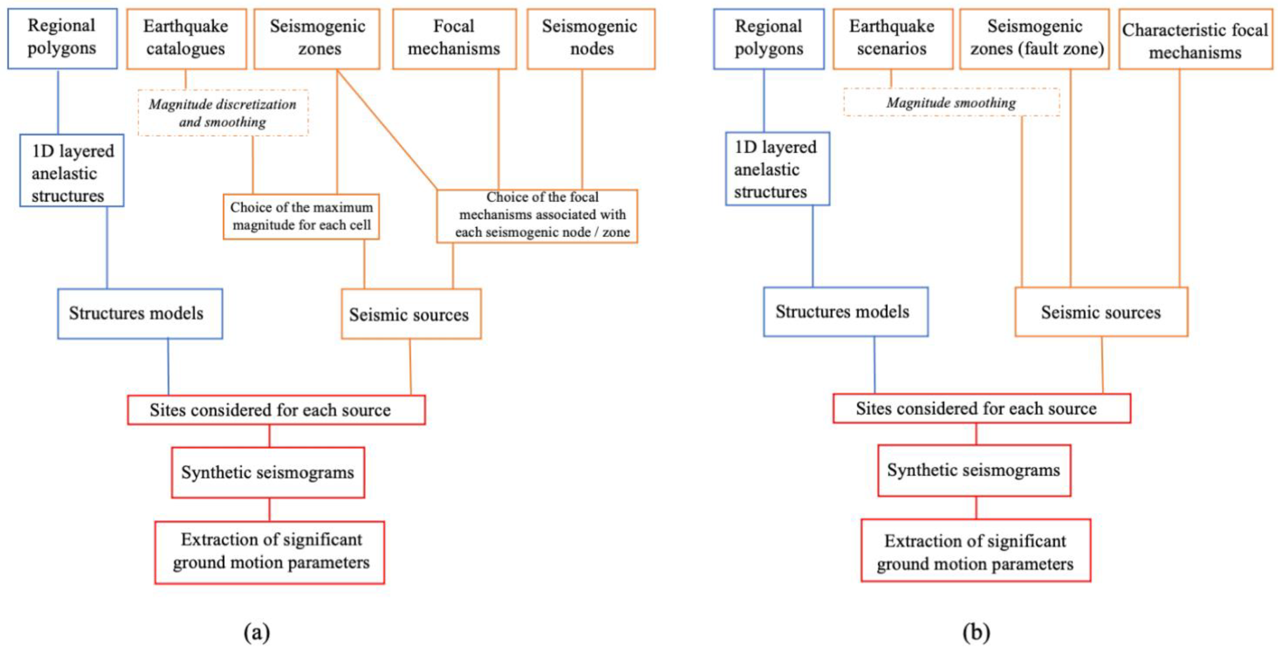
3. NDSHA Approach: Methodology

The history and detailed technical description of NDSHA has been reviewed in several publications, e.g., [32,43,44,51,53,54]. The Neo-deterministic Seismic Hazard Assessment (NDSHA) originated in 1996 [55], and was seen as a response to several drawbacks of Probabilistic Seismic Hazard Analysis (PSHA) widely used in the world [49]. NDSHA does not need to use Gutenberg-Richter relation in that it considers enveloping earthquake scenarios and may include the Maximum Credible Earthquake (MCE) in the computations [44]. Different from standard PSHA and classical DSHA [56], NDSHA does not rely on the use of empirical attenuation relations and a limited set of scenario earthquakes, but starts from basic physics and takes into consideration the mechanical properties of earthquake sources and pathways to compute realistic synthetic seismograms and to depict the hazard level at the sites of interest (e.g., [32]). Since 1996, the neo-deterministic approach has undergone several rehearsals and improvements (e.g., [32,43,44,51,53,57,58]). It has been developed as a comprehensive multi-disciplinary approach for performing multi scenario-based seismic hazard computations based on all available geophysical-geological-tectonic information, and could be applied from national to local scale [33].
Although it is a young method compared with PSHA, NDSHA is being extensively applied and tested in many countries since a couple of decades, e.g., Croatia [59], Kosovo [60], northern Morocco [61], Egypt [62], India [58,63], North China [64], Southwest China [45]. As shown in Figure 3a, the standard computation scheme contains a wealth of deterministic inputs, such as historical and instrumental earthquake catalogues, seismogenic nodes, seismogenic zones, focal mechanisms, and regional polygons equipped with characteristic structural models (mechanical properties) are the input datasets for standard NDSHA computations. For the purposes of computing the hazard database (described in Section 4.2), it is essential to adjust and simplify the standard procedure, as shown in Figure 3b. In particular, the input datasets consist of earthquake scenarios, i.e., a given focal mechanism for each of the predefined 0.2° × 0.2° seismogenic zones, and regional polygons equipped with characteristic structural models. Both the standard and the ad hoc computational schemes adopt the same core methodology: (1) efficient computation of realistic broadband synthetic seismograms are made by means of the modal summation method [32,65,66]; (2) regional polygons representing different structural models are used to account for the natural complexity of the Earth’s structure—here, we used the datasets defined in [45]; (3) the study area is gridded into 0.2° × 0.2° cells; (4) the earthquake catalogue has been discretized with 0.2° × 0.2° grid and then smoothed to account for the epicentral location error and for the finite dimension of seismic sources [32]; (5) all the gridded sources defined in (4) are used in the computation of synthetic seismograms.
As shown in Figure 3b, in the computational schemes adapted for EEW2.0, the earthquake scenarios are smoothed to account for the finite dimension of seismic sources and uncertainty of earthquake location. In the standard NDSHA computation for regional scale, the areas without historical earthquakes recorded are filled with M ≥ 5.0 earthquake scenarios instead. In our case, we define a large seismogenic zone containing the whole fault zone, and choose not to fill the “blank” area with M ≥ 5.0 earthquake scenarios. Thereupon, in each computation, only one (smoothed) source will be used as the input to the computation of synthetic seismograms.

4. EEW2.0

The EEW2.0 is endowed with two characters: (1) the earthquake scenarios are the first basic input information and the possible hazard (MMI) maps for all possible earthquake scenarios are comprehensively considered; (2) differentiated alerts are provided for different end-users. The main procedure for implementing such a system contains (a) the classification of an earthquake, and its damaging potential from magnitude; (b) a hazard database composed of a set of MMI maps for different magnitude classes; (c) a decision framework for alert notification to different protected objects.

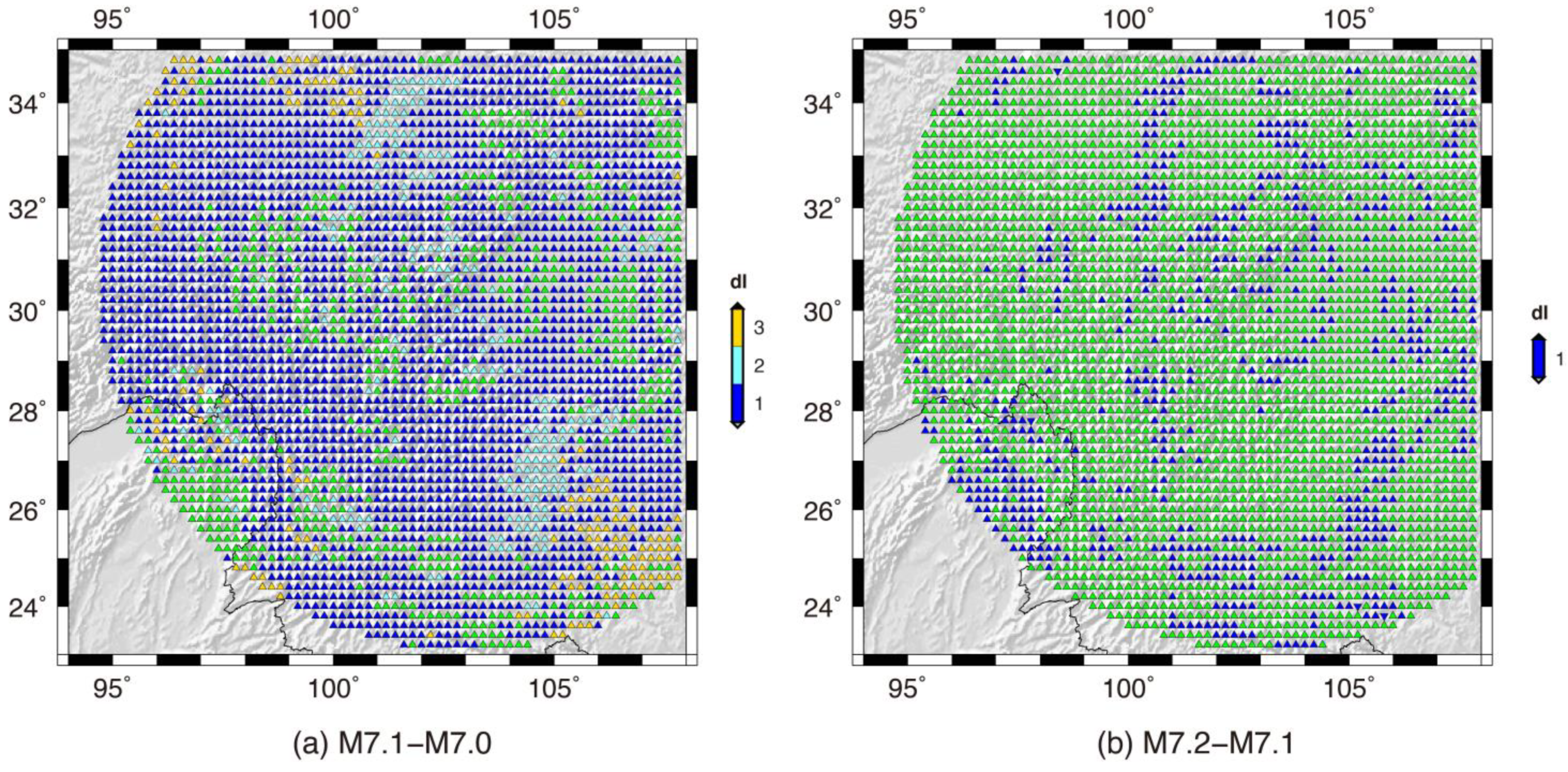
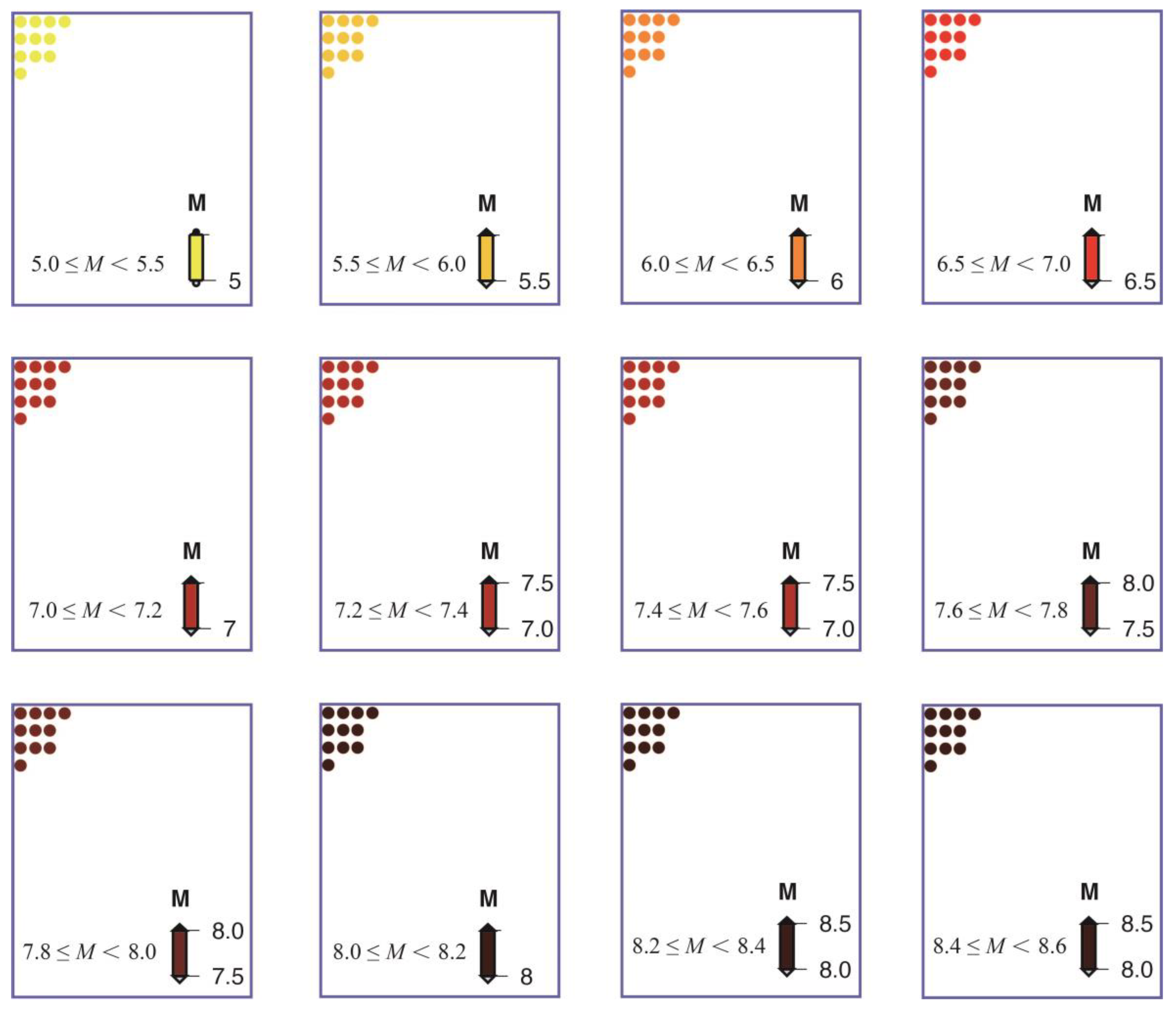
4.1. Simple Classification of Earthquakes, and Their Damaging Potential, from Magnitude

In order to delineate the difference in “potential to cause hazard” for earthquakes with different magnitude, eight scenario computations were performed using the size scaled point source (SSPS) approximation [43], considering M = 6.0, M = 6.2, M = 6.5, M = 6.7, M = 7.0, M = 7.1, M = 7.2, M = 7.5, with the other parameters (epicenter, depth, strike, dip, rake) fixed. The comparison of the results obtained with M = 7.0 and M = 6.5 shows that the differences in the MMI values are smaller than 2 Intensity units (i.e., ∆I < 2. For any macroseismic scale is defined by ordinal integer (discrete) numbers. The artifact of introducing half-values of Intensity is consistent with the quite arbitrary statement by [67]: “On a scale with 12 degrees, intensity can usually be estimated with a precision of about half a degree”. The sentence violates the definition of intensity scale: “A sequence of Natural Ordinal Number, i.e., a scale in which each number tells the position of something in a discrete scale of integers, such as I, II, III, IV, V, etc.”), whereas in the comparison between M = 7.5 and M = 7.0, ∆I = 4 can be reached (Figure 4). When comparing the results for M = 6.7 and M = 6.5, M = 7.0 and M = 6.7, ∆I < 2, whereas for M = 7.2 and M = 7.0, ∆I = 4 can be reached. For M = 7.5 and M = 7.2, ∆I = 3 can be reached, but only in tiny areas (Figure 5). When comparing the results for M = 7.1 and M = 7.0, M = 7.2 and M = 7.1, ∆I = 3 can be reached (Figure 6). According to the tests above, two conclusions can be drawn: (1) for magnitudes smaller than 7.0, ∆I < 2 when ∆M 0.5; (2) for magnitudes larger or equal than 7.0, ∆I = 3 can be reached even if ∆M = 0.1. Thus, for M < 7, 0.5 could regarded as the minimum interval to be used in the grouping of magnitudes for prognostic evaluations. In general, magnitude uncertainty is 0.2–0.3 [68,69,70]. Thus, for 7.0  M < 8.0 and 8.0  M < 8.6, 0.2 could be regarded as the minimum interval.
The existing classification for magnitude and earthquake effects (http://www.geo.mtu.edu/UPSeis/magnitude.html, accessed on 14 August 2021), i.e., minor (3.0~3.9), light (4.0~4.9), moderate (5.0~5.9), strong (6.0~6.9), major (7.0~7.9) and great (8.0 or larger) earthquake is obviously not suitable for our purposes. Therefore, according to the results described so far, the magnitude ranges from 5.0 to 8.6 have been divided into the 12 classes listed in Table 2, which correspond to a quite smooth class transition and minimize boundary effects.

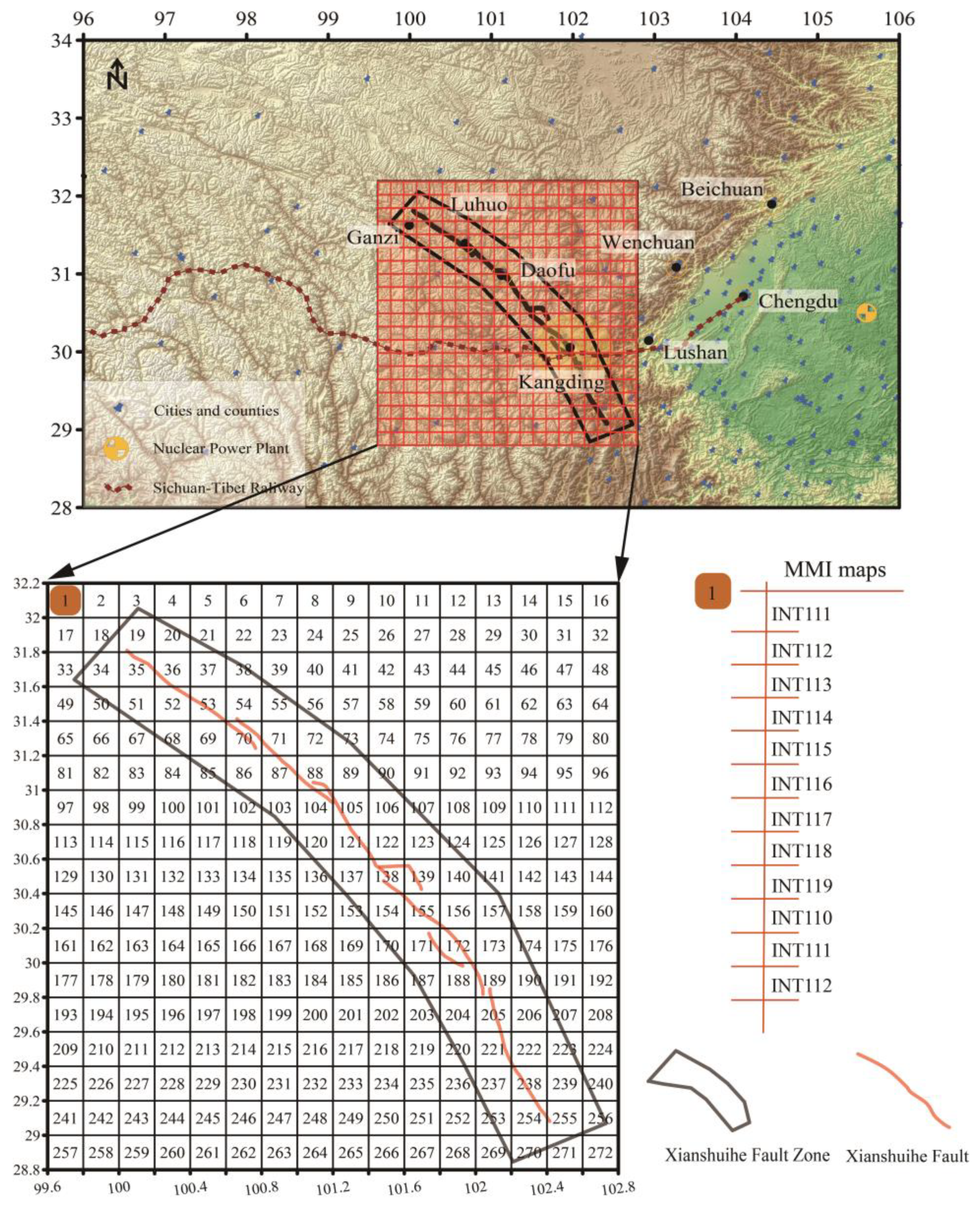
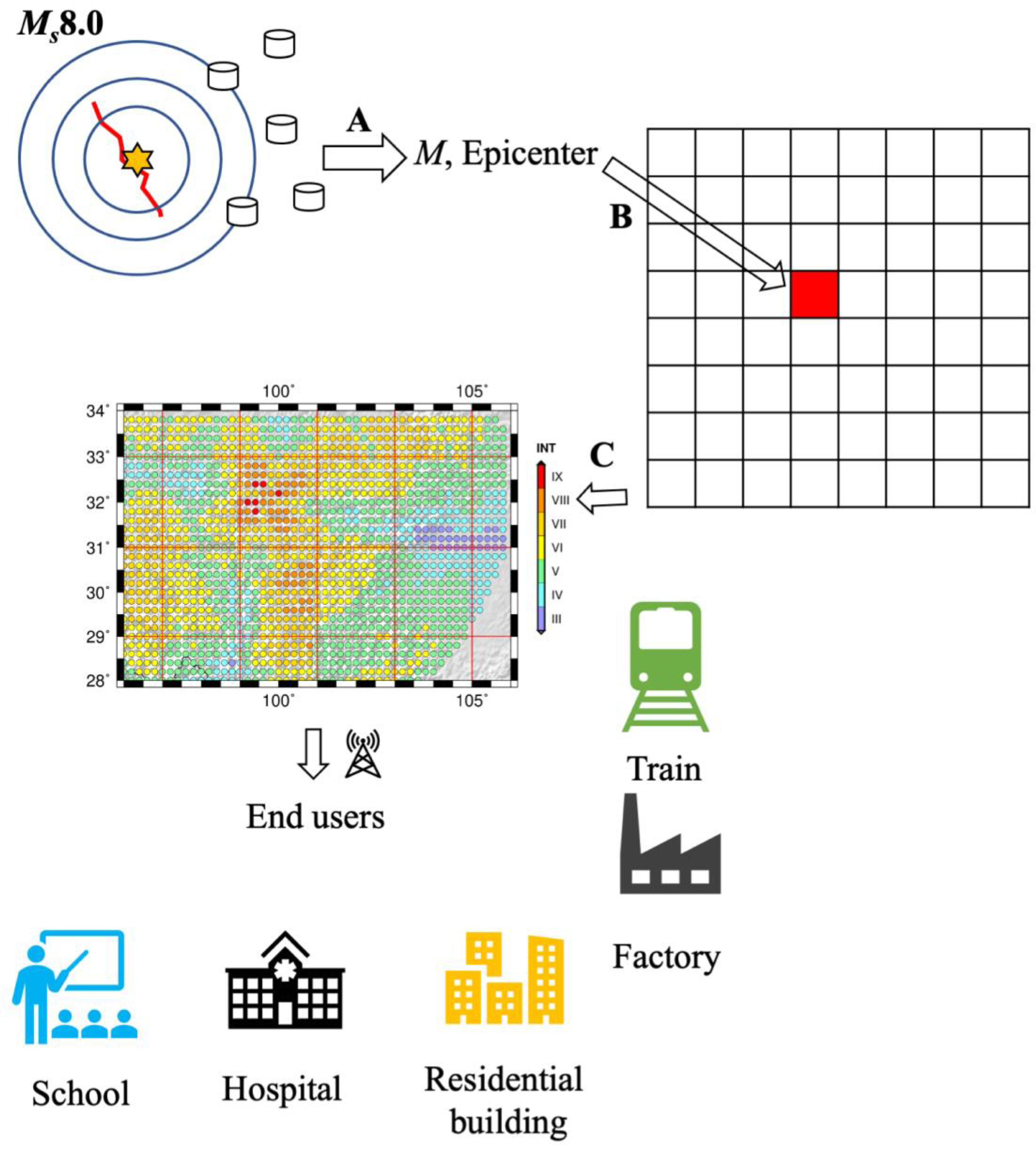
4.2. Hazard Database: MMI Maps

As shown in Figure 7, the colored “squares” delineate a 0.2 ° × 0.2 ° grid; the same rule applied in NDSHA for the discretization and smoothing of seismicity, covering the whole XSH. Then, to each cell in the grid an identification number is assigned. For each cell, 12 NDSHA computations are performed following the magnitude classification given in Table 2. The results are finally transformed into MMI maps, and to each MMI map a unique code is also assigned.
The detailed procedures followed to build a MMI database in the test area is given in Figure 7, assuming that the red grid area contains all possible seismic sources linked to XSH. In our test, we assume that all those potential earthquakes linked to XSH are included in the red rectangle covering the whole XSH. Supposing that one forgets an important password, the simplest way to retrieve the forgotten password is just to try all possible combinations (e.g., for a six-number password, there are 106 possible combinations) at the simple cost of spending some time. Similarly, though, we cannot precisely predict the location and size of the next damaging earthquake linked to XSH, we can consider all the relevant possible sizes (M 5.0) and locations of potential earthquakes according with now-available geophysical datasets, and then model all the possible ground motion values at the simple cost of using more memory and computing resources.
To optimize the size of the MMI database, we apply the same rules adopted to determine the focal depth ( h d ) of earthquakes with different magnitudes in standard regional computations (e.g., [45]), i.e., h d = 10 for M < 7 ; h d = 15 for 7 M < 8 ; h d = 25 for M 8 . In general, an M = 5.0 earthquake is considered a damaging earthquake (Table 3). The maximum magnitude can be effectively defined by earthquake forecast/prediction algorithms (e.g., [71,72]) and morpho-structural analysis [35]. From the result of the ongoing M8 Time of Increased Probability (TIP) experiment, the maximum magnitude in XSH could exceed 8.0 [71]. As shown by [44], a Mdesign = 8.7 was used in each seismogenic node prone to great earthquakes and only one node is included (Figure 7). Following the source gridding rule, in the source area there are 16 × 17 = 272   0.2 ° × 0.2 ° cells (Figure 7). For example, the cells numbered 1st~16th occupy the first row, 17th~32nd occupy the second row, and the last cell is the 272nd. In order to take all possible earthquake scenarios into consideration, 12 simplified regional computations are performed in 272 cells, with the following procedures:
(1)
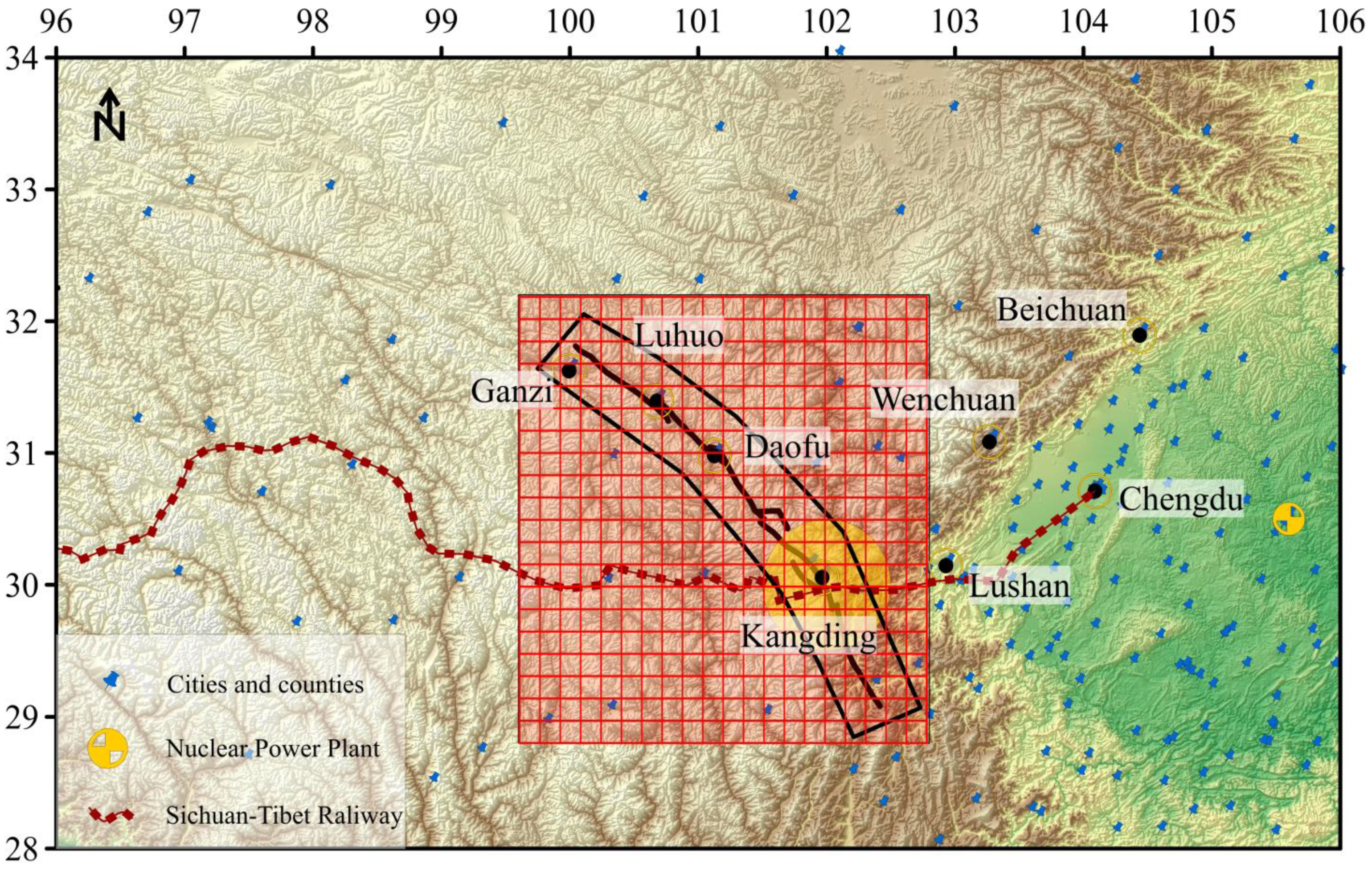
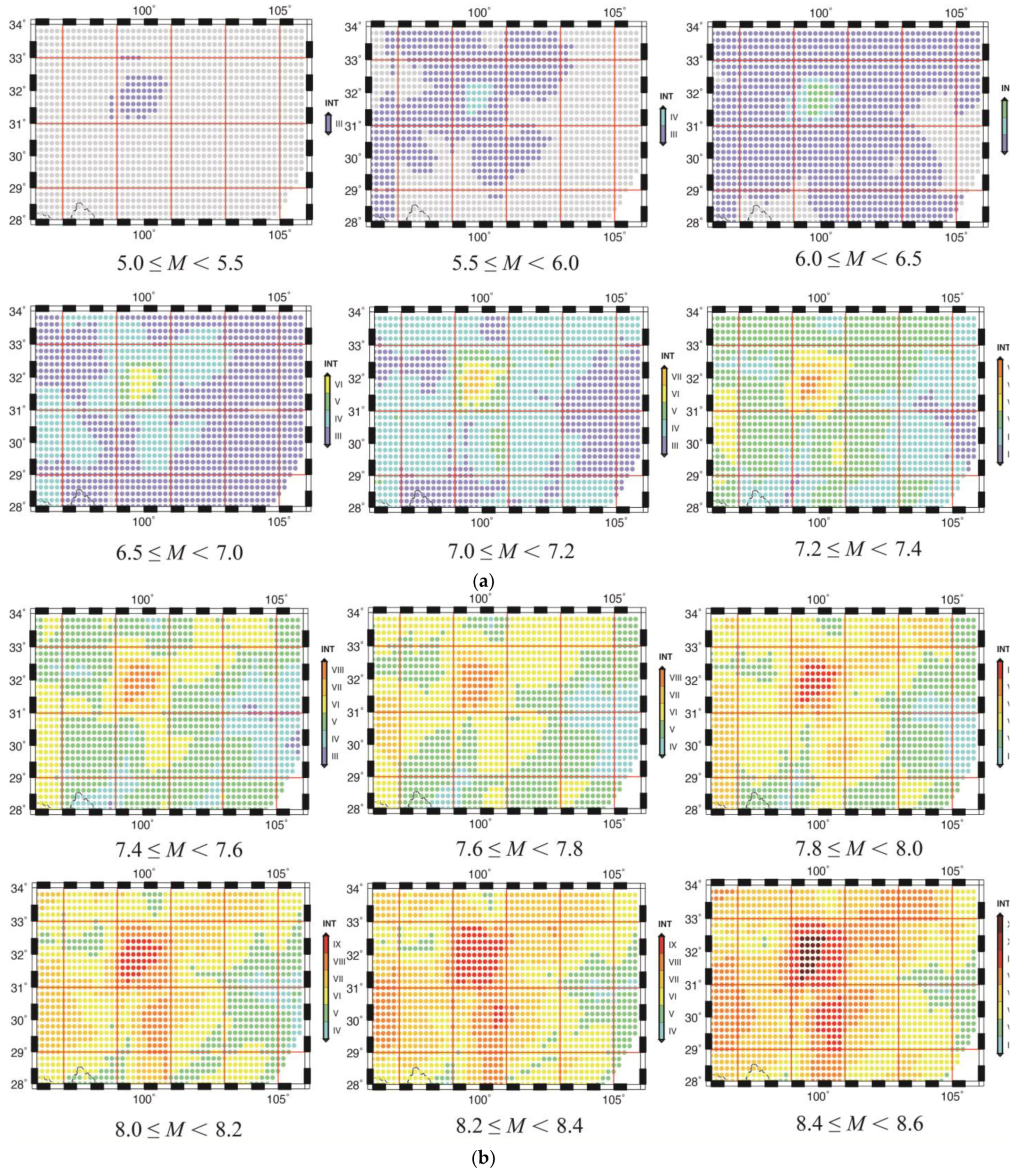
The seismogenic zone is defined by the coordinates 99.6°~102.8° E, 28.8°~32.2° N, i.e., the whole XSH.
(2)
The source is placed in the first cell (99.6°~99.8° E, 32.0°~32.2° N), and its magnitude is set as 5.0.
(3)
All the 272 (smoothed) sources related with XSH are characterized, for simplification of computing procedures, by the same rupture and the focal mechanism characteristic of XSH (strike = 146°, dip = 82°, rake = 349°).
(4)
The predefined 0.2° × 0.2° cellular grid, corresponding to the cellular structural models referenced by [45], is adopted for the computation of synthetic seismograms at the sites.
(5)
For the same source cell defined in (2), the value of magnitude is changed to the next class, and the depth is defined following the predefined rules, iterating for the next 11 (up to the final magnitude class) regional computations in (3).
(6)
The magnitude is reset to 5.0 (and the depth to 10 km), the source is moved to the 2nd source cell (99.8°~100.0° E, 32.0°~32.2° N), and steps (2)–(4) are repeated.
Finally, after finishing the computations above, one will obtain 3264 results, i.e., 3264 MMI maps for 3264 earthquake scenarios. The detailed description of the exploitation of the MMI database is shown in Figure 8 and its caption.
Following the computational scheme described in Section 3, we briefly describe here an example for the 1st cell, including 12 computations. The sources to be used for the computation of synthetic seismograms in these 12 computations are shown in Figure 9. Each source is smoothed, with a radius of three cells, to account for its extension in space and the error in its localization [32,73], which is hereafter called cellular source. In each computation, the value of magnitude is defined as the lower limit of the corresponding magnitude class, e.g., M is defined as 5.0 in the magnitude class IA ( 5.0 M < 5.5 ) in the first computation in 1st grid. The results (i.e., MMI maps) of these 12 computations are shown in Figure 10a,b. For the sake of covering the whole study area and controlling the number of computed synthetic seismograms, the maximum epicentral distance was set at 600 km. These 12 computations in 1st grid cost about 1 h (2009 Xserve with eight cores/16 threads 2.26 GHz CPU) and take about 6 GB disk space. The whole computation will occupy about 3 TB disk space.

4.3. Decision Framework for Alert Notification

The end-users are the basic concern of EEW2.0. For any EEW system to be effective, it is essential to publicize its principles, purposes and technical limitations to general public [10].
If, for example, a Ms 7.5 happens and the warning alert is rapidly sent to a town, but the general population does not understand the meaning of the warning alert, just a few resulting emergence responses are activated: the earthquake still severely affects the normal life in the town. This situation may be more common in the countries and regions where EEW is progressing or planning. For the effective protection of lives and reduction in damages and losses, it is mandatory to consider potential damages and losses, and to compare them with losses caused by false alarms. For example, a factory owner may be more interested in the comparison between the losses resulting from downtime (production interruption) after receiving an alert and the losses resulting from damages resulting from ignoring the alert. Accordingly, it is necessary to differentiate warning alert to different end-users at different sites or situations, so that they could have suitable emergence responses to the alert, e.g., a surgery room cannot ignore an IMMI = 5 alert because slight ground motion could still severely influence the high resolution and complex surgery, but a school designed against IMMI = 6 could ignore it and continue its normal actions in a short time.
Here, we propose a decision framework for end-users to determine whether or not to actively respond to a warning alert, as shown in Figure 11. In general, the purpose of minimizing the influence from an earthquake could be divided as follows: (a) maximize the safety of individuals; (b) minimize the economy losses. In order to maximize the safety of individuals, one needs to consider the minimization of the number of deaths and injuries. In order to minimize the economic losses, one needs to consider the possible costs of repair and restoration, and the costs caused by factory downtime. Overall, it is a complex procedure to comprehensively decide whether or not to respond to a warning alert from an earthquake.

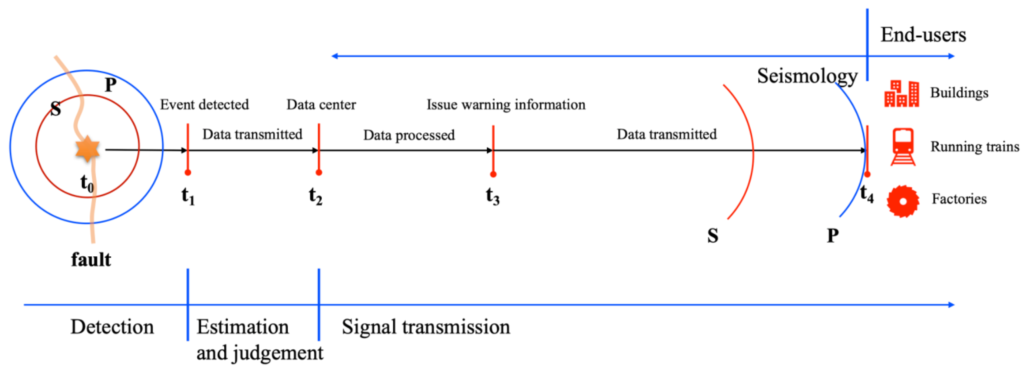
4.4. Conceptual Working Mechanism

One possible conceptual view of EEW2.0 is shown in Figure 12: the warning is expected to be issued once the first wavefront reaches the boundary of protected areas. R1 is the distance between the epicenter and the closest station. R2 is the radius of the blind zone (i.e., the distance that seismic wave travels in the time it takes to detect and process seismic signals until the magnitude and epicenter are determined). The grid stands for the protected area by the early warning alert. Each yellow point stands for the a priori computed MMI value at each site. Indicating the average P-wave velocity with Vp and the average S-wave velocity with Vs, and the epicenter distance to one targeted site with EDI (i.e., the thick black line in the figure), the theoretical leading time Twt (i.e., ignoring the time delay that may be caused by data processing, transmission, etc.), in each site of the protected area is:
T w t = E D I ( 1 / V s 1 / V p ) T d e t e c t T p r o c e s s i n g .
T d e t e c t is the time needed at the closest station to detect the earthquake signal and T p r o c e s s i n g is the time needed to estimate magnitude and epicenter. Due to the fact that the epicentral distance for each site is different, the leading time at each site is also different. However, it is possible for each site to receive the warning alert at the same time in a zero-latency [74]. One possible application scenario of EEW2.0 is shown in Figure 13. Fast estimation of magnitude and epicenter will rapidly trigger the EEW2.0 system; by quickly matching to the prepared MMI database labeled by location range (epicenter) and magnitude class, the warning alert can be rapidly sent to different end-users based on the extracted precomputed MMI map.

5. Discussion and Conclusions

Through the rapid detection and signal processing after a damaging earthquake happened, EEW may provide valuable information for the public in the areas vulnerable to significant ground motions. The lead time, a few to tens of seconds before the arrival of damaging S waves, provided by such an emergence response mechanism, could play an essential role in saving lives and protecting properties. Thus, EEW, to some extent, is a tool for emergency responses to earthquakes. A similar example is the interception of missiles by the Air Defense System (ADS), where the function of ADS is the same of EEW and a detected offensive missile plays the role of a suddenly occurred earthquake. It is truly a strategic choice to decide where to deploy ADS since one system cannot protect the whole country. Similarly, it is a seismological choice to decide where to deploy an EEW, and SHA provides important information for making such a decision. Thus, it is necessary and possible to combine EEW and SHA.
Considering the peculiarities of NDSHA, its combination with EEW may be developed into two settings: (1) regional SHA tells EEW where the dangerous area is, and then EEW is deployed in that specific area; (2) regional SHA has told EEW where the dangerous area is, and then the adoption of prepared MMI maps (obtained by NDSHA computations considering all possible earthquake scenarios) is a component of EEW in alerting the public. In this paper, we limited the discussion of the second setting, assuming XSH as the dangerous area (in fact, it is a dangerous area according to previous NDSHA results); the first setting will be the topic of a forthcoming paper.
Actually, the most important purpose in EEW is to decrease processing time and increase the lead-time. We propose that EEW2.0 (empowered by NDSHA) provides different warning alerts to various sites (end-users). Such an action requires three steps: (1) to test the non-linear relationship between “potential to cause hazard” and magnitude; (2) to divide the magnitude ranging from 5.0 to 8.6 into 12 classes; (3) to explain how to build an MMI-based hazard database and manage it.
Although EEW2.0 is still not yet implemented in practice, it already suggests new possibilities for future progresses of EEW, and confirms the usefulness of NDSHA in solidly estimating seismic hazard. As more attention is put into the reduction in seismic activity and its secondary risks, the proposed EEW2.0 will likely play an important role in protecting lives, reducing losses, and improving the efficiency of EEW.

Author Contributions

In the framework of an international cooperation between Department of Mathematics and Geosciences, University of Trieste, and China Seismic Experimental Site, the present idea was an output of a collaborative effort by all co-authors. All authors have read and agreed to the published version of the manuscript.

Funding

The work was supported, on the Chinese side, by the Special Fund of China Seismic Experimental Site [grant No. 2019CSES0101] and the National natural Science Foundation of China (NSFC) [grant No. U2039207].

Data Availability Statement

Not applicable.

Acknowledgments

We would like to express our sincere thanks to Polly Chen, the assistant editor of MDPI Wuhan, for providing us the chance to publish our work about EEW2.0, a possible next-generation EEW empowered by NDSHA. We also want to express special thanks to the Department of Mathematics and Geosciences, University of Trieste, for providing technology of NDSHA and computing resources for carrying this challenging test out. Part of the computations have been made using the XeRiS facilities (http://www.xeris.it/WebApp/, accessed on 9 November 2021). VGK thanks the Russian Science Foundation for support of the scenario approach in seismic hazard assessment (RSCF Project No. 20-17-00180).

Conflicts of Interest

The authors declare that they have no known competing financial interests or personal relationships that could have appeared to influence the work reported in this paper.

References

  1. Cooper, J.D. San Francisco Daily Evening Bulletin. 1868. Available online: https://spectrum.ieee.org/a-brief-history-of-earthquake-warnings (accessed on 18 November 2021).
  2. Heaton, T.H. A model for a Seismic Computerized Alert Network. Science 1985, 228, 987–990. [Google Scholar] [CrossRef] [Green Version]
  3. Ben-Menahem, A. A concise history of mainstream seismology: Origins, legacy and perspectives. Bull. Seismol. Soc. Am. 1995, 85, 1202–1225. Available online: https://pubs.geoscienceworld.org/ssa/bssa/article-abstract/85/4/1202/102637/A-concise-history-of-mainstream-seismology-Origins (accessed on 29 September 2021).
  4. Wenzel, F.; Baur, M.; Fiedrich, F.; Lonescu, C.; Lonescu, M.C. Potential of earthquake early warning systems. Nat. Hazards 2001, 23, 407–416. [Google Scholar] [CrossRef]
  5. Erdik, M.; Fahjan, Y.; Ozel, O.; Alcik, H.; Mert, A.; Gul, M. Istanbul Earthquake Rapid Response and the Early Warning System. Bull. Earthq. Eng. 2003, 1, 157–163. [Google Scholar] [CrossRef]
  6. Xu, Y.; Burton, P.W.; Tselentis, G.A. Regional seismic hazard for Revithoussa, Greece: An earthquake early warning Shield and selection of alert signals. Nat. Hazards Earth Syst. Sci. 2003, 3, 757–776. [Google Scholar] [CrossRef] [Green Version]
  7. Allen, R.M.; Kanamori, H. The potential for earthquake early warning in southern California. Science 2003, 300, 786–789. [Google Scholar] [CrossRef] [Green Version]
  8. Espinosa-Aranda, J.M.; Cuellar, A.; Rodriguez, F.H.; Frontana, B.; Ibarrola, G.; Islas, R.; Garcia, A. The seismic alert system of Mexico (SASMEX): Progress and its current applications. Soil Dyn. Earthq. Eng. 2011, 31, 154–162. [Google Scholar] [CrossRef]
  9. Lancieri, M.; Fuenzalida, A.; Ruiz, S.; Madariaga, R. Magnitude scaling of early-warning parameters for the Mw 7.8 Tocopilla, Chile. Bull. Seism. Soc. Am. 2011, 101, 447–463. [Google Scholar] [CrossRef] [Green Version]
  10. Kamigaichi, O.; Saito, M.; Doi, K.; Matsumori, T.; Tsukada, S.; Takeda, K.; Shimoyama, T.; Nakamura, K.; Kiyomoto, M.; Watanabe, Y. Earthquake early warning in Japan: Warning the general public and future prospects. Seismol. Res. Lett. 2009, 80, 717–726. [Google Scholar] [CrossRef]
  11. Nakamura, H.; Horiuchi, S.; Wu, C.J.; Yamamoto, S.; Rydelek, P.A. Evaluation of the real-time earthquake information system in Japan. Geophys. Res. Lett. 2009, 36, L00B01. [Google Scholar] [CrossRef] [Green Version]
  12. Fujinawa, Y.; Noda, Y. Japan’s earthquake early warning system on 11 March 2011: Performance, shortcomings and changes. Earthq. Spectra 2013, 29, 341–368. [Google Scholar] [CrossRef]
  13. Picozzi, M.; Zollo, A.; Brondi, P.; Colombelli, S.; Elia, L.; Martino, C. Exploring the feasibility of a nationwide earthquake early warning system in Italy. J. Geophys. Res. Solid Earth 2015, 120, 2446–2465. [Google Scholar] [CrossRef]
  14. Iannaccone, G.; Zollo, A.; Elia, L.; Convertito, V.; Satriano, C.; Martino, C.; Festa, G.; Lancieri, M.; Bobbio, A.; Stabile, T.A.; et al. A prototype system for earthquake early-warning and alert management in southern Italy. Bull. Earthq. Eng. 2010, 8, 1105–1129. [Google Scholar] [CrossRef] [Green Version]
  15. Satriano, C.; Elia, L.; Martino, C.; Lancieri, M.; Zollo, A.; Lannaccone, G. PRESTo, the earthquake early warning system for Southern Italy: Concepts, capabilities and future perspectives. Soil Dyn. Earthq. Eng. 31, 137–153. [CrossRef] [Green Version]
  16. Heidari, R.; Shomali, Z.H.; Ghayamghamian, M.R. Magnitude-scaling relations using period parameters tau(c) and tau(max)(p), for Tehran region, Iran. Geophys. J. Int. 2013, 192, 275–284. [Google Scholar] [CrossRef] [Green Version]
  17. Enferadi, S.; Shomali, Z.H.; Niksejel, A. Feasibility study of earthquake early warning in Tehran, Iran. J. Seismol. 2021, 25, 1127–1140. [Google Scholar] [CrossRef]
  18. Picozzi, M.; Bindi, D.; Pittore, M.; Kieling, K.; Parolai, S. Real-time risk assessment in seismic early warning and rapid response: A feasibility study in Bishkek (Kyrgyzstan). J. Seism. 2013, 17, 485–505. [Google Scholar] [CrossRef]
  19. Kanamori, H. The diversity of the physics of earthquakes. Proc. Jpn. Acad. Ser. B Phys. Biol. Sci. 2004, 80, 297–316. [Google Scholar] [CrossRef] [Green Version]
  20. Rundle, J.; Stein, S.; Donnellan, A.; Turcotte, D.L.; Klein, W.; Saylor, C. The complex dynamics of earthquake fault systems: New approaches to forecasting and nowcasting of earthquakes. Rep. Prog. Phys. 2021, 84, 076801. [Google Scholar] [CrossRef]
  21. Kanamori, H. Real-time seismology and earthquake damage mitigation. Annu. Rev. Earth Planet. Sci. 2005, 33, 195–214. [Google Scholar] [CrossRef] [Green Version]
  22. Wu, Y.M.; Kanamori, H. Development of an Earthquake Early Warning System using real-time strong motion signals. Sensors 2008, 8, 1–9. [Google Scholar] [CrossRef] [PubMed] [Green Version]
  23. Horiuchi, S.; Horiuchi, Y.; Yamamoto, S.; Nakamura, H.; Wu, C.J.; Rydelek, P.A.; Kachi, M. Home seismometer for earthquake early warning. Geophys. Res. Lett. 2009, 36, L00B04. [Google Scholar] [CrossRef] [Green Version]
  24. Minson, S.E.; Brooks, B.A.; Glennie, C.L.; Murray, J.R.; Langbein, J.O.; Owen, S.E.; Heaton, T.H.; Lannucci, R.A.; Hauser, D.L. Crowdsourced earthquake early warning. Sci. Adv. 2015, 1, e1500036. [Google Scholar] [CrossRef] [Green Version]
  25. Wang, Y.; Li, S.Y.; Song, J.D. Threshold-based evolutionary magnitude estimation for an earthquake early warning system in the Sichuan-Yunnan region, China. Sci. Rep. 2020, 10, 21055. [Google Scholar] [CrossRef]
  26. Hilbring, D.; Titzschkau, T.; Buchmann, A.; Bonn, G.; Wenzel, F.; Hohnecker, E. Earthquake early warning for transport lines. Nat. Hazards 2014, 70, 1795–1825. [Google Scholar] [CrossRef]
  27. Pagano, L.; Sica, S. Earthquake early warning for earth dams: Concepts and objectives. Nat. Hazards 2013, 66, 303–318. [Google Scholar] [CrossRef]
  28. Cheng, M.H.; Wu, S.; Heaton, T.H.; Beck, J.L. Earthquake early warning application to buildings. Eng. Struct. 2014, 60, 155–164. [Google Scholar] [CrossRef]
  29. Kubo, T.; Hisada, Y.; Murakami, M.; Kosuge, F.; Hamano, K. Application of an earthquake early warning system and a real-time strong motion monitoring system in emergency response in a high-rise building. Soil Dyn. Earthq. Eng. 2011, 31, 231–239. [Google Scholar] [CrossRef]
  30. Maruyama, Y.; Yamazaki, F.; Sakaya, M. Experiments of earthquake early warning to Expressway Drivers using synchronized driving simulators. Earthq. Spectra 2009, 25, 347–360. [Google Scholar] [CrossRef] [Green Version]
  31. Cremen, G.; Galasso, C. Earthquake early warning: Recent advances and perspective. Earth Sci. Rev. 2020, 205, 103184. [Google Scholar] [CrossRef]
  32. Panza, G.F.; Romanelli, F.; Vaccari, F. Seismic wave propagation in laterally. heterogeneous anelastic media: Theory and application to seismic zonation. Adv. Geophys. 2001, 43, 1–95. [Google Scholar] [CrossRef]
  33. Panza, G.F.; Kossobokov, V.G.; Laor, E.; De Vivo, B. Earthquakes and Sustainable Infrastructure: Neodeterministic (NDSHA) Approach Guarantees Prevention Rather than Cure, 1st ed.; Elsevier: Amsterdam, The Netherlands, 2021; ISBN 978-0-12-823503-4. [Google Scholar]
  34. Deng, Q.D.; Zhang, P.Z.; Ran, Y.K.; Yang, X.P.; Min, W.; Chen, L.C. Active tectonics and earthquake activities in China. Earthq. Sci. Front. 2003, 10, 66–73, (In Chinese with English abstract). [Google Scholar]
  35. Gorshkov, A.; Kossobokov, V.; Soloviev, A. Recognition of earthquake-prone areas. In Nonlinear Dynamics of the Lithosphere and Earthquake Prediction; Vladimir, K.B., Soloviev, A.A., Eds.; Springer: Berling/Heidelberg, Germany, 2003; pp. 239–310. ISBN 978-3-662-05298-3. [Google Scholar]
  36. Satriano, C.; Wu, Y.M.; Zollo, A.; Kanamori, H. Earthquake early warning: Concepts, methods and physical grounds. Soil Dyn. Earthq. Eng. 2011, 31, 106–118. [Google Scholar] [CrossRef]
  37. Allen, M.R.; Melgar, D. Earthquake Early Warning: Advances, scientific challenges, and societal Needs. Annu. Rev. Earth Planet. Sci. 2019, 47, 361–388. [Google Scholar] [CrossRef] [Green Version]
  38. Velazquez, O.; Pescaroli, G.; Cremen, G.; Galasso, C. A review of the technical and socio-organizational components of earthquake early warning systems. Front. Earth Sci. 2020, 8, 533498. [Google Scholar] [CrossRef]
  39. Oliveira, C.S.; de Sa, F.M.; Lopes, M.; Ferreira, M.A.; Pais, I. Early warning systems: Feasibility and end-users’ point of view. Pure Appl. Geophys. 2015, 172, 2353–2370. [Google Scholar] [CrossRef]
  40. Xu, H. Minimizing the ripple effect caused by operational risks in a make-to-order supply chain. Int. J. Phys. Distrib. Logist. Manag. 2020, 50, 381–402. [Google Scholar] [CrossRef]
  41. Wu, Y.M.; Kanamori, H. Rapid assessment of damage potential of earthquakes in Taiwan from the beginning of P waves. Bull. Seism. Soc. Am. 2005, 95, 1181–1185. [Google Scholar] [CrossRef] [Green Version]
  42. National Research Council. Living on an Active Earth: Perspectives on Earthquake Science; National Academies Press: Cambridge, MA, USA, 2003; ISBN 978-0309065627. [Google Scholar]
  43. Panza, G.F.; La Mura, C.; Peresan, A.; Romanelli, F.; Vaccari, F. Seismic hazard scenarios as preventive tools for a disaster resilient society. Adv. Geophys. 2012, 53, 93–165. [Google Scholar] [CrossRef]
  44. Rugarli, P.; Vaccari, F.; Panza, G.F. Seismogenic nodes as a viable alternative to seismogenic zones and observed seismicity for the definition of seismic hazard at regional scale. Vietnam J. Earth Sci. 2019, 41, 289–304. [Google Scholar] [CrossRef] [Green Version]
  45. Zhang, Y.; Romanelli, F.; Vaccari, F.; Peresan, A.; Jiang, C.S.; Wu, Z.L.; Gao, S.H.; Kossobokov, G.V.; Panza, G.F. Seismic hazard maps based on Neo-deterministic Seismic Hazard Assessment for China Seismic Experimental Site and its adjacent areas. Eng. Geol. 2020, 291, 106208. [Google Scholar] [CrossRef]
  46. Fahjan, Y.M.; Alcik, H.; Sari, A. Applications of cumulative absolute velocity to urban earthquake early warning systems. J. Seismol. 2011, 15, 355–373. [Google Scholar] [CrossRef]
  47. McGuire, R.K. Probabilistic seismic hazard analysis: Early history. Earthquake Engng Struct. Dyn. 2008, 37, 329–338. [Google Scholar] [CrossRef]
  48. Gasparini, P.; Manfredi, G.; Zschau, J. Earthquake early warning as a tool for improving society’s resilience and crisis response. Soil Dyn. Earthq. Eng. 2011, 31, 267–270. [Google Scholar] [CrossRef]
  49. Wyss, M.; Nekrasova, A.; Kossobokov, V. Errors in expected human losses due to incorrect seismic hazard estimates. Nat. Hazards 2012, 62, 927–935. [Google Scholar] [CrossRef]
  50. Panza, G.; Kossobokov, V.G.; Peresan, A.; Nekrasova, A. Chapter 12: Why are the standard probabilistic methods of estimating seismic hazard and risks too often wrong. In Earthquake Hazard, Risk and Disasters; Academic Press: Cambridge, MA, USA, 2014; pp. 309–357. ISBN 978-0-12-394848-9. [Google Scholar]
  51. Panza, G.F.; Bela, J. NDSHA: A new paradigm for reliable seismic hazard assessment. Eng. Geol. 2020, 275, 105403. [Google Scholar] [CrossRef]
  52. Panza, G.F.; Bela, J. Reliable seismic hazard assessment: NDSHA. Albanian J. Nat. Tech. Sci. 2021, 26, in press. [Google Scholar]
  53. Bela, J.; Panza, G.F. NDSHA—The new paradigm for RSHA—An updated review. Vietnam J. Earth Sci. 2021, 43, 111–188. [Google Scholar] [CrossRef]
  54. Panza, G.F. NDSHA: Robust and Reliable Seismic Hazard Assessment. Proceedings of International Conference on Disaster Risk Mitigation, Dhaka, Bangladesh, 23–24 September 2017. [Google Scholar]
  55. Panza, G.F.; Vaccari, F.; Costa, G.; Suhadolc, P.; Fäh, D. Seismic input modeling for zoning and microzoning. Earthquake Spectra 1996, 12, 529–566. [Google Scholar] [CrossRef]
  56. Reiter, L. Earthquake Hazard Analysis: Issues and Insights; Columbia University Press: New York, NY, USA, 1990; ISBN 978-0231513203. [Google Scholar]
  57. Peresan, A.; Zuccolo, E.; Vaccari, F.; Gorshkov, A.; Panza, G.F. Neo-deterministic seismic hazard and pattern recognition techniques: Time-dependent scenarios for North-Eastern Italy. Pure Appl. Geophys. 2011, 168, 583–607. [Google Scholar] [CrossRef]
  58. Parvez, I.A.; Vaccari, F.; Panza, G.F. A deterministic seismic hazard map of India and adjacent areas. Geophys. J. Int. 2003, 155, 489–508. [Google Scholar] [CrossRef]
  59. Markušić, S.; Suhadolc, P.; Herak, M.; Vaccari, F. A contribution to seismic hazard assessment in Croatia from deterministic modeling. In Seimic Hazard of the Circum-Pannonian Region; Panza, G., Radulian, M., Trifu, C., Eds.; Birkhauser Verlag: Basel, Switzerland, 2000; ISBN 978-3-0348-8415-0. [Google Scholar]
  60. Brandmayr, E.; Vaccari, F.; Romanelli, F.; Vlahovic, G.; Panza, G.F. Neo-deterministic seismic hazard maps of Kosovo. Vietnam J. Earth Sci. 2021, 43, 1–10. [Google Scholar] [CrossRef]
  61. Mourabit, T.; Abou Elenean, K.M.; Ayadi, A.; Benouar, D.; Ben Suleman, A.; Bezzeghoud, M.; Cheddadi, A.; Chourak, M.; ElGabry, M.N.; Harbi, A.; et al. Neo-deterministic seismic hazard assessment in North Africa. J. Seismol. 2014, 18, 301–318. [Google Scholar] [CrossRef]
  62. El-Sayed, A.; Vaccari, F.; Panza, G.F. Deterministic seismic hazard in Egypt. Geophys. J. Int. 2001, 144, 555–567. [Google Scholar] [CrossRef] [Green Version]
  63. Parvez, I.A.; Magrin, A.; Vaccari, F.; Ashish; Mir, R.; Peresan, A.; Panza, G.F. Neo-deterministic seismic hazard scenarios for India—A preventive tool for disaster mitigation. J. Seismol. 2017, 21, 1559–1575. [Google Scholar] [CrossRef]
  64. Ding, Z.F.; Vaccari, F.; Chen, Y.T.; Panza, G.F. Deterministic seismic hazard map in North China. In Earthquake Hazard, Risk, and Strong Ground Motion; Chen, Y.T., Panza, F.G., Wu, Z.L., Eds.; Seismological Press: Beijing, China, 2004; pp. 351–360. ISBN 7-5028-2506-1. [Google Scholar]
  65. Panza, G.F. Synthetic seismograms: The Rayleigh waves modal summation. J. Geophys. 1985, 58, 125–145. [Google Scholar]
  66. Florsch, N.; Fäh, D.; Suhadolc, P.; Panza, G.F. Complete synthetic seismograms for high-frequency multimode SH-waves. Pure Appl. Geophys. 1991, 136, 529–560. [Google Scholar] [CrossRef]
  67. Kárník, V.; Algermissen, S.T. Seismic zoning. In The Assessment and Mitigation of Earthquake Risk. NICI; United Nations Educational, Scientific and Cultural Organization: Paris, France, 1978; pp. 11–47. ISBN 92-3-101451-X. [Google Scholar]
  68. Båth, M. Introduction to Seismology; Birkhäuser Verlag: Basel, Switzerland, 1973. [Google Scholar]
  69. Chung, I.A.; Henson, I.; Allen, M.R. Optimizing Earthquake Early Warning Performance: ElarmS-3. Seism. Res. Lett. 2019, 90, 727–743. [Google Scholar] [CrossRef] [Green Version]
  70. Bormann, P.; Liu, R.F.; Ren, X.; Gutdeutsch, R.; Kaiser, D.; Castellaro, S. Chinese National Network magnitudes, their relation to NEIC magnitudes, and recommendations for new IASPEI magnitude standards. Bull. Seismol. Soc. Am. 2007, 97, 114–127. [Google Scholar] [CrossRef]
  71. Ismail-Zadeh, A.; Kossobokov, V. Earthquake prediction, M8 Algorithm. In Encyclopedia of Solid Earth Geophysics; Gupta, H.K., Ed.; Springer: Amsterdam, The Netherlands, 2020; pp. 1–5. ISBN 978-90-481-8702-7. [Google Scholar]
  72. Kossobokov, V. Earthquake prediction: 20 years of global experiment. Nat. Hazards 2013, 69, 1155–1177. [Google Scholar] [CrossRef]
  73. Panza, G.F.; Prozorov, A.; Suhadolc, P. Is there a correlation between lithosphere structure and statistical properties of seismicity? Terra Nova 1990, 2, 585–595. [Google Scholar] [CrossRef]
  74. Minson, S.E.; Meier, M.A.; Baltay, A.S.; Hanks, T.C.; Cochran, E.S. The limits of earthquake early warning: Timeliness of ground motion estimates. Sci. Adv. 2018, 4, eaaq0504. [Google Scholar] [CrossRef] [PubMed] [Green Version]
Figure 1. The study area of EEW2.0. The red grid, covering 99.6°~102.8° (E) and 28.8°~32.2° (N), shows the area where the scenario earthquakes are considered. The irregular black polygon enclosing part of the red cells stands for the Xianshuihe Fault Zone (XSH). The black lines stand for segments of XSH [34]. It can be clearly seen that the red grid covers the four vertices of the irregular polygons surrounding XSH. The yellow circle stands for the seismogenic node prone to M 8.2 earthquakes [35]. The blue pushpins stand for the residential areas, and Chengdu, Lushan, Kangding, Wenchuan, Beichuan, Daofu, Luhuo, and Ganzi are indicated by black dots. The approximate location of the planned Sanba Nuclear Power Plant is marked by a pierced yellow circle. The approximate location of the Sichuan-Tibet railway is also displayed.
Geosciences 11 00473 g001
Figure 2. The timeline of an earthquake early warning (EEW) system (adopted from [36,39]).
Geosciences 11 00473 g002
Figure 3. NDSHA computation scheme: (a) standard procedures; (b) adjust procedures.
Geosciences 11 00473 g003
Figure 4. The differences of MMI values obtained considering computations of four scenarios with varying magnitude values (magnitude step is equal to 0.5) whereas the other focal parameters are fixed. Distribution of differences between (a) magnitude 7 and 6.5, and (b) magnitude 7.5 and 7.0 scenario computations. The green triangles indicate the different is zero.
Geosciences 11 00473 g004
Figure 5. The differences of MMI values obtained considering computations of four scenarios with varying magnitude values (magnitude step is equal to 0.2/0.3) whereas the other focal parameters are fixed. Distribution of differences between (a) magnitude 6.7 and 6.5, (b) magnitude 7.0 and 6.7, (c) magnitude 7.2 and 7.0, and (d) magnitude 7.5 and 7.2. The green triangles indicate the different is zero.
Geosciences 11 00473 g005
Figure 6. The differences of MMI values obtained from four scenarios with varying levels of magnitude (magnitude step is equal to 0.1), whereas the other focal parameters are fixed. Distribution of differences between (a) magnitude 7.1 and 7.0, and (b) magnitude 7.2 and 7.1 scenario computations. The green triangles indicate the different is zero.
Geosciences 11 00473 g006
Figure 7. Study area with “protected” and “seismogenic” zone (28.8°~32.2° N, 99.6°~102.8° E) meshed by 0.2° × 0.2° grid. For each cell of the protected area, 12 MMI maps are computed.
Geosciences 11 00473 g007
Figure 8. The framework of MMI Database (MMID, shortened as ID) to be used in the EEW2.0. The establishment of an integrated ID could be divided into three steps: (1) Grid the whole protected area with 0.2° × 0.2° grids; (2) assign a unique label to each cell, i.e., CEmn, 1≤m, n≤16, and m, n are always integers. For example, CE11 stands for the cell at the first row and the first column, and CE1338 stands for the cell at the 13th row and the 38th column. (3) At each cell, two fields are assigned. The first field is location, including the longitude and latitude range; the second field is the classification of magnitudes. For example, in the cell CE11, the classification of magnitudes includes four classes, i.e., M1, M2, M3, M4 (maybe more, in practice). Each magnitude class refers to a unique prepared MMI result labeled by INTmnX, matching the unique MMI result prepared for the Xth magnitude class in the cell at the mth row and the nth column, e.g., assumed an M = 7.0 earthquake occurred in CE11, and 7 is in M3 class, then the earthquake could quickly match the prepared MMI result INT113 in the MMI database.
Geosciences 11 00473 g008
Figure 9. The sources to be used in the 12 scenario computations, with a different value of magnitude for each cellular earthquake source. For each scenario computation, the value of magnitude is defined as the lower limit of the corresponding magnitude, e.g., the adopted magnitude for computing MMI map is 5.0 for the 5.0 ≤ M < 5.5 class.
Geosciences 11 00473 g009
Figure 10. (a) The 1 to 6 MMI maps for the cellular source scenario 1 shown in Figure 9. (b) The 7 to 12 MMI maps for the cellular source scenario 1 shown in Figure 9.
Geosciences 11 00473 g010
Figure 11. Suggested decision framework for the end-user (i.e., a factory in this case) to determine whether to issue an alert after an earthquake is detected.
Geosciences 11 00473 g011
Figure 12. The conceptual view of EEW2.0. The red solid circle located in (1,1) stands for the epicenter, and R1 is the distance between the epicenter and the closest station. R2 is the radius of the blind zone (i.e., the distance that seismic wave travels in the time it takes to detect and process seismic signals until the magnitude and epicenter are determined). The rectangle filled with orange circles, in 0.2° × 0.2° cells, stands for the protected area. Assuming the average P-wave velocity is Vp and the S-wave velocity is Vs, and the epicenter distance to one target site is EDI (i.e., the thick black line in the figure), the warning time Twt in each cell is: Twt = EDI ∗ (1⁄Vs − 1⁄Vp) − TdetectTprocessing. Tdetect means the time needed at the closest station to detect the earthquake signal and Tprocessing is the time needed to estimate magnitude and epicenter. The orange circles stand for the precomputed Modified Macroseismic Intensity (MMI) by NDSHA (e.g., [43]).
Geosciences 11 00473 g012
Figure 13. One possible application scenario of MMI database: (A) Fast estimation of magnitude and epicenter; (B) fast matching of the cell including the epicenter and the magnitude class; (C) extraction from the MMI database of the pertinent MMI maps and issue of the warning to different end users, e.g., school, hospital, residential building, factory, and train.
Geosciences 11 00473 g013
Table 1. Comparison between Earthquake Early Warning and Seismic Hazard Assessment tools.
Earthquake Early WarningSeismic Hazard Assessment Tools (PSHA, NDSHA)
PurposesReduction in Seismic Risk
Time lengthAfter earthquakes, a few seconds to a few tens of seconds [46]Before earthquakes, long- to intermediate-term prediction (PSHA: ≥50 years, e.g., [47]; NDSHA: from a few years to tens of years, e.g., [43])
InputFirst seconds of primary P wavesHistorical earthquake catalogue, seismogenic zones, structural models (only for NDSHA), focal mechanism (only for NDSHA), seismogenic nodes (only for NDSHA)
OutputLead time and estimated ground motion valuesSeismic hazard in terms of probabilistic-based or deterministic-based ground motion values
AdvantagesPrepare time for emergence responsesPrepare descriptions for future seismic hazard distribution
DisadvantagesMissed or false alarms [48], blind zonesUnderestimation and nonphysical-based (PSHA, e.g., [49])
Table 2. Magnitude classes used in computing MMI database. Each class could be simply expressed as XX, where the first X stands for I, II, and III, and the second X stands for A, B, C, D, and E. For example, IA refers to the magnitude class 5.0 ≤ M < 5.5.
Class I :   5.0 M < 7.0 II :   7.0 M < 8.0 III :   M 8.0
A 5.0 M < 5.5 7.0 M < 7.2 8.0 M < 8.2
B 5.5 M < 6.0 7.2 M < 7.4 8.2 M < 8.4
C 6.0 M < 6.5 7.4 M < 7.6 8.4 M < 8.6
D 6.5 M < 7.0 7.6 M < 7.8
E 7.8 M < 8.0
Table 3. Earthquake magnitude classes ranging from minor to great.
ClassMagnitudeEarthquake Effects
Minor3.0~3.9May be felt
Light4.0~4.9Likely felt
Moderate5.0~5.9Minor damage may occur
Strong6.0~6.9Damage may occur
Major7.0~7.9Damage expected
Great8.0 or largerSignificant damage expected
Publisher’s Note: MDPI stays neutral with regard to jurisdictional claims in published maps and institutional affiliations.

