When Enough Is Really Enough? On the Minimum Number of Landslides to Build Reliable Susceptibility Models

Abstract

Mapping existing landslides is a fundamental prerequisite to build any reliable susceptibility model. From a series of landslide presence/absence conditions and associated landscape characteristics, a binary classifier learns how to distinguish potentially stable and unstable slopes. In data rich areas where landslide inventories are available, addressing the collection of these can already be a challenging task. However, in data scarce contexts, where geoscientists do not get access to pre-existing inventories, the only solution is to map landslides from scratch. This operation can be extremely time-consuming if manually performed or prone to type I errors if done automatically. This is even more exacerbated if done over large geographic regions. In this manuscript we examine the issue of mapping requirements for west Tajikistan where no complete landslide inventory is available. The key question is: How many landslides should be required to develop reliable landslide susceptibility models based on statistical modeling? In fact, for such a wide and extremely complex territory, the collection of an inventory that is sufficiently detailed requires a large investment in time and human resources. However, at which point of the mapping procedure, would the resulting susceptibility model produce significantly better results as compared to a model built with less information? We addressed this question by implementing a binomial Generalized Additive Model trained and validated with different landslide proportions and measured the induced variability in the resulting susceptibility model. The results of this study are very site-specific but we proposed a very functional protocol to investigate a problem which is underestimated in the literature.

1. Introduction

Landslide susceptibility assessment is the most common approach to assess how prone a given landscape is to generate landslides. At the scale of a single slope this is commonly achieved by solving geotechnical relations that express the equilibrium of a potential unstable mass [1,2]. For broader geographic contexts, i.e., from catchments to regional and even continental scales, landslide susceptibility is commonly generated via data-driven or expert-driven methods. Expert-driven models are based on the standardization and weighting of causative factor maps, even without the availability of a sufficiently complete landslide inventory. Data-driven methods use binary classifiers, of a statistical or machine learning origin. Irrespective of the specific algorithm at hand, certain conditions need to be met for a data-driven-based susceptibility assessment. The first condition is to have access to a series of spatially-explicit instances describing landslides that have already occurred. Under the assumption that “the past is the key to the future” [3], the model learns how to discriminate landslide presences from the absences on the basis of a set of predisposing factors. Any classifier, essentially, measures the correlations existing among the proportion of presence/absence data and the range or classes described by each predisposing factor under consideration. Due to this, variations in the distribution and proportion of presence/absence data have an impact on the model results. Some articles have already investigated this effect. The first attempt was made by Guzzetti et al. [4], who assessed the variation in model performance as the input data changed by randomly sub-sampling the whole number of mapping units available in their study area. A mapping unit corresponds to the basic geographic objects in which a study area is partitioned and to which probability values of landslide occurrence are assigned to Guzzetti et al. [4] concluded that the random sampling did not have any major effect on the proportion of stable and unstable units, which remained relatively constant for the replicates they produced. A similar conclusion was later reached by Heckmann et al. [5] who tested a similar assumption but adding a step where the size of the dataset changed while contextually checking auto-correlation issues as many susceptibility replicas were built. Frattini et al. [6] initially constrained the input data, combining an equal amount of mapping units with absence and presence of landslides. They highlighted variations in the model performance as the proportion of absences became increasingly unbalanced. This topic was further investigated in several contributions such as Van Den Eeckhaut et al. [7], Petschko et al. [8], Conoscenti et al. [9], Lombardo and Mai [10].

It must be highlighted that all the scientific efforts mentioned above were carried out by keeping the presence information essentially constant and varying the number of the absence instances putted into the model. This is clearly a reasonable assumption because it is important to use as much landslide data as possible in building the best susceptibility model. Fewer articles have tested the implications of varying the presence conditions. This specific topic involves a slightly different scientific domain, where the research question is related to the effects of incomplete inventories onto the resulting susceptibility map [11], which means also investigating the minimum requirement with respect to landslide data in order to be able to use data-driven models at all.

In this case, the thread linking the scientific research gravitates around landslide positional errors [12] or the missing information of landslide presences at certain locations [13]. The common denominator among these is to assess the effect of incomplete landslide inventories and test approaches aimed at removing the bias induced by the incompleteness, from an optimal reference model [14].

From this particular setting we took inspiration for the present work. However, instead of seeking ways to adjust a model built on the basis of a less numerous landslide inventory, here we pose a different key question: When would a model built on a small number of landslides be sufficiently capable to describe the landslide susceptibility theoretically obtained by training a model on the basis of a much larger dataset, without any specific bias adjustment? The reason for such a question is the fact that in data scarcity situations [15], it is very common to have limited information on the distribution of landslides [16], and globally, it is very common to hardly have access to any landslide data at all [17]. Therefore, mapping landslides is a mandatory step without which no data-driven susceptibility model could be built in these areas [18,19].

More specifically, in the context of the research project ‘Silk Road Disaster Risk Reduction’, aimed at assessing unstable slopes along the new silk road (Belt and Road Initiative) [20], the already existing landslide inventories in this famous pathway are very limited. Based on the landslide susceptibility evaluation carried out at a continental scale in central Asia, Titti et al. [21] show the necessity to build more detailed susceptibility models at a national scale even where national scale landslide inventories are not available or very incomplete at best. Considering the vast area and the complexity of the mountainous landscape in the countries of central Asia, to map a complete landslide inventory would take a very long time.

In this context we tried to answer our key question, evaluating the landslide susceptibility in Tajikistan applying several constraints. At the beginning of this work, a limited number of landslide inventories were already available in the study area. To safely consider a landslide inventory that is enough populated to support our analysis, we decided to integrate the existent catalogs with an intense landslide mapping activity from satellite images that required long additional time, after which, we assumed the inventory to be reliable (see Figure 1). Then, the analysis was carried out, reducing the number of presence cases in our dataset and actually converted them to absences, mimicking a situation where we did not know that landslides were there. After that, we compared the effect of an increasingly smaller number of landslide presences to a landslide susceptibility model built by using a binomial Generalized Additive Model [22,23,24], implemented in INLA [25,26,27]. INLA is an R [28] package developed by Lindgren and Rue [29] that allows users to implement a number of statistical models in a Bayesian framework, providing analogous and much faster results than traditional MCMC [30,31].

2. Materials and Methods

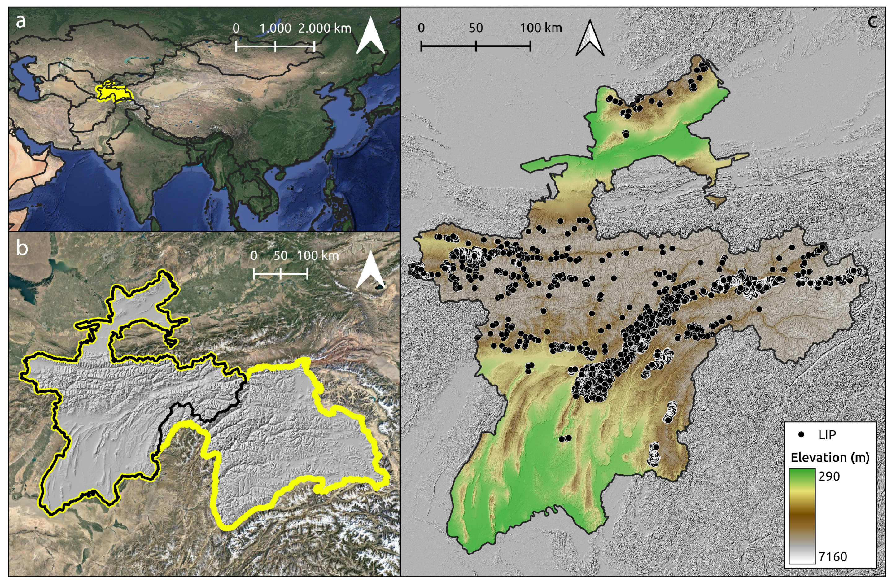
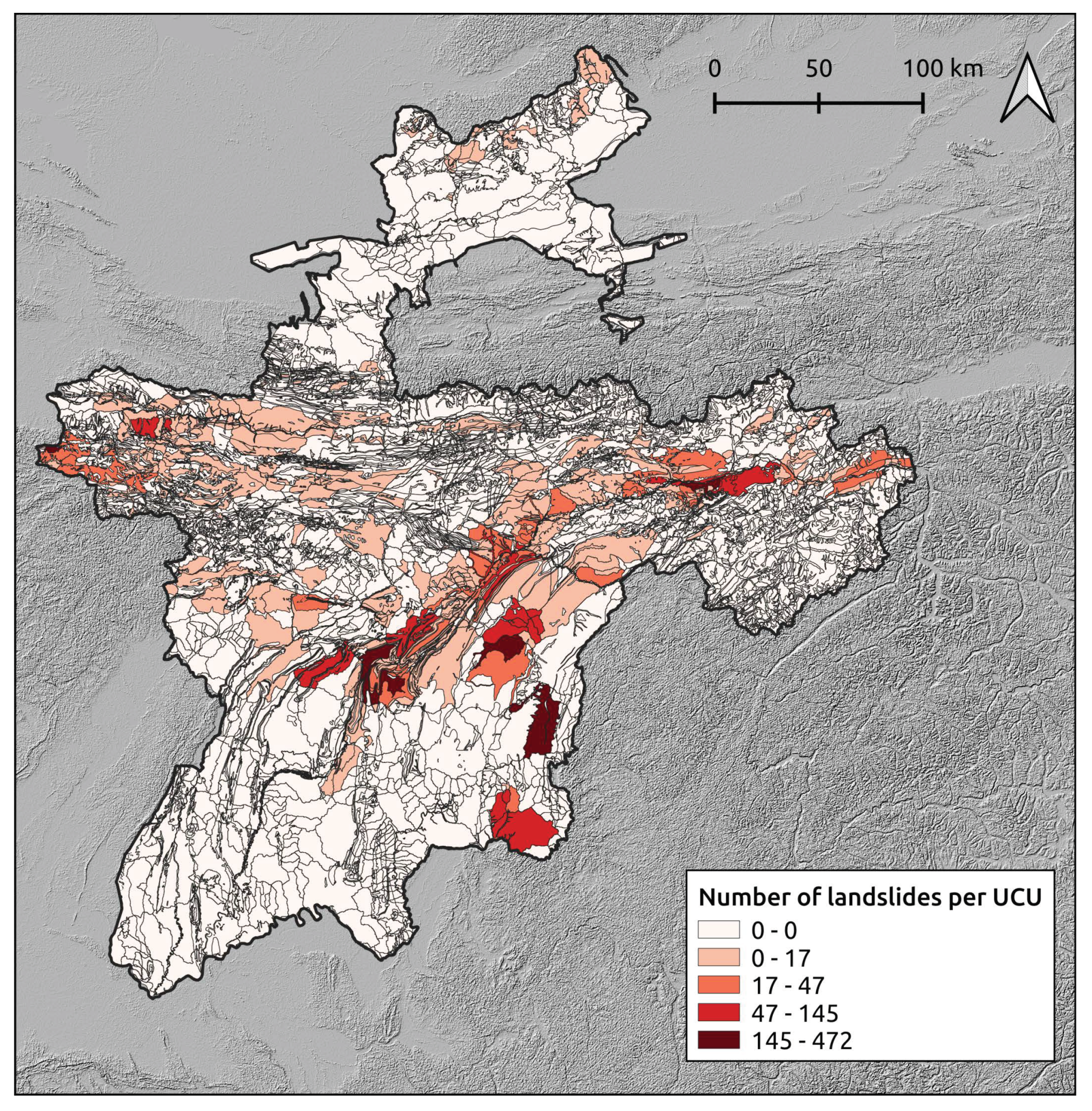
2.1. Tajikistan and Its Reference Landslide Inventory

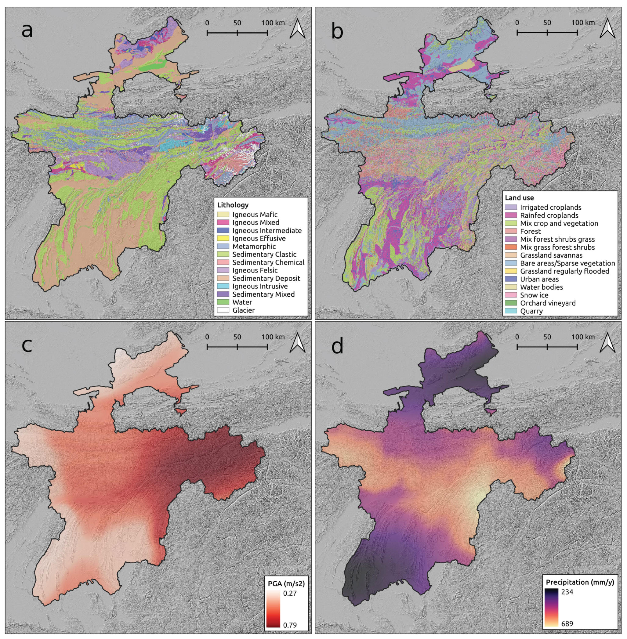
Tajikistan is characterized by an extremely complex rough terrain, with approximately 44% of its territory potentially hosting permafrost, which is rapidly thawing [32]. Thick soils with a relatively high erodibility index [33] characterize the area. In conjunction with these peculiarities, high intensity precipitation affects the whole territory and strong earthquakes have been reported throughout the history of the country. This combination makes Tajikistan particularly prone to landslides. Shallow and fast landslides are mainly visible in Tajikistan, such as debris slides and debris flows.

Numerous examples of earthquake-induced landslides [34,35,36], rainfall-induced ones [37,38,39], and a combination of both effects exist [40]. This has even produced the highest landslide dam in the world [41] after a coseismic failure.

Due to the large area of the country, we focused on the western part, excluding the eastern region of Gorno-Badakhshan, which is characterized by the presence of numerous glaciers and by the very low density of population and infrastructure.

Geologically, the western part of Tajikistan is extremely complex, with 12% of its lithologies being of igneous origins, 11% metamorphic, 72% sedimentary, and 3% covered by glaciers (see Figure 2a). In terms of land use, the anthropic control on the natural environment is very limited, with relatively small pockets of croplands and large areas with bare land or sparse vegetation (see Figure 2b).

As for the main landslide triggers, the strongest seismic activity is registered in the central eastern regions, partly overlapping with the areas with the highest amount of rainfall (see Figure 2c,d).

Landslides were mapped as individual points, without any attributes on the classification with respect to type and age, focusing on the initiation areas. Some information has been collected from Havenith et al. [35], Nazirova and Saidov [42], and others have been mapped using image interpretation from Google Earth Images. In addition to this, we used the earthquake-induced landslide inventories for some of the historical earthquakes (e.g., the Khait earthquake 1949) [36,43]. Each point representative of a landslide was assigned to the highest point along the landslide crown. We chose this representation instead of the common alternative of a centroid (see [44]) because of the shallow nature of the recognized landslides. This is in fact the most conservative choice in case of shallow flow-like landslides although a laboratory test have also highlighted that the same processes can also exhibit a marked retrogressive behavior (e.g., [45]). Nevertheless, due to the relatively coarse size of the mapping unit we chose (see Section 2.3), the models we tested would not be sensitive to either point representation criteria. In other words, both the centroid or the highest point along the landslide crown would fall within the same mapping unit, thus labeled as unstable for the following analyses.

2.2. Covariates

Nine morphometrical, seismic, and meteorological covariates were selected and pre-processed (see

Table 1. Covariates used in the analysis, types, acronyms, and units.

Covariate	Original Type	Acronym	Unit
Slope degree	Continuous	Slope	degree (°)
Relative relief	Continuous	Rlf	m
Plan curvature	Continuous	PlC	${\mathrm{m}}^{-1}$
Profile curvature	Continuous	PrC	${\mathrm{m}}^{-1}$
Peak Ground Acceleration	Continuous	PGA	$\mathrm{m}/{\mathrm{s}}^2$
Annual precipitation	Continuous	Rn	mm/y
Land use	Categorical	LU	unitless
Lithology	Categorical	Litho	unitless
Area with Slope > 10° per map unit	Continuous	Area	${\mathrm{m}}^2$

), seven of which are continuous and two categorical.

Relative relief, slope degree, plan curvature (curvature tangent to the contour line), and profile curvature (curvature tangent to the slope line) have been derived from the 30-m Shuttle Radar Topography Mission (SRTM) DEM [46]. The former has been calculated as the range between the maximum and minimum elevation in a neighborhood of 1 km of radius, the others using the formula by Zevenbergen and Thorne [47].

The annual rainfall map is the result of the cumulative daily precipitation of one year averaged over 10 years of data (2010–2019). The precipitation data was obtained from the Multi-Satellite Retrievals for Global Precipitation Measure (IMERG) [48] with a cell size of 10 × 10 km.

The PGA has been mapped with the 475-year Return Period by Ischuk et al. [49].

Lithology provided by the Tajikistan General Office of Geology [50], which has been classified into 13 classes (see Figure 2a) and Land use in 14 classes (see Figure 2b).

Grid-cells with a slope steepness less than 10 degrees were masked out before computing any of the covariates mentioned above, as these were considered a priori as not being susceptible to landslide initiation. Before any susceptibility analyses was run, a mean zero, unit variance rescaling procedure was applied to all numerical variables.

2.3. Mapping Units

Different methods may be used to obtain the terrain objects in which a given study area is partitioned. In the landslide susceptibility literature, these objects commonly consist of grid cells, terrain units, Unique Condition Units (UCUs), slope units, geo-hydrological units, topographic units, and administrative units [51].

To evaluate the landslide susceptibility in Tajikistan, the study area was subdivided into mapping units that take into account the landslides predisposing factors according to the concept of the Unique Condition Unit (UCU) [52,53]. The reason behind such a choice was meant to partition the study area into spatial object that are as independent as possible from the adjacent once while respecting the natural hydrological, geomorphological, and geological structure of the landscape under consideration. This is particularly relevant in case of statistical models, for they assume independence among each instance of the target variable.

Specifically, we intersected a catchment partition (obtained via ’r.watersheds’ in QGIS) with the lithology map (scale 1:2,800,000). This operation produced 16,020 UCUs with a maximum size of 738 km ${}^2$. These UCUs were assigned with a binary status 1/0 according to the presence/absence of landslides. After this operation, 677 UCUs contained at least one landslide and 15,343 were considered stable (Figure 3).

As for the covariate information associated to each of the UCUs, we opted to summarize the distribution of each continuous parameter via its mean and standard deviation (with the exception of the area). Conversely, the categorical covariates have been expressed in terms of the predominant class per UCU. Overall, this operation led to the generation of 15 covariates. Their specific use within the model will be explained below.

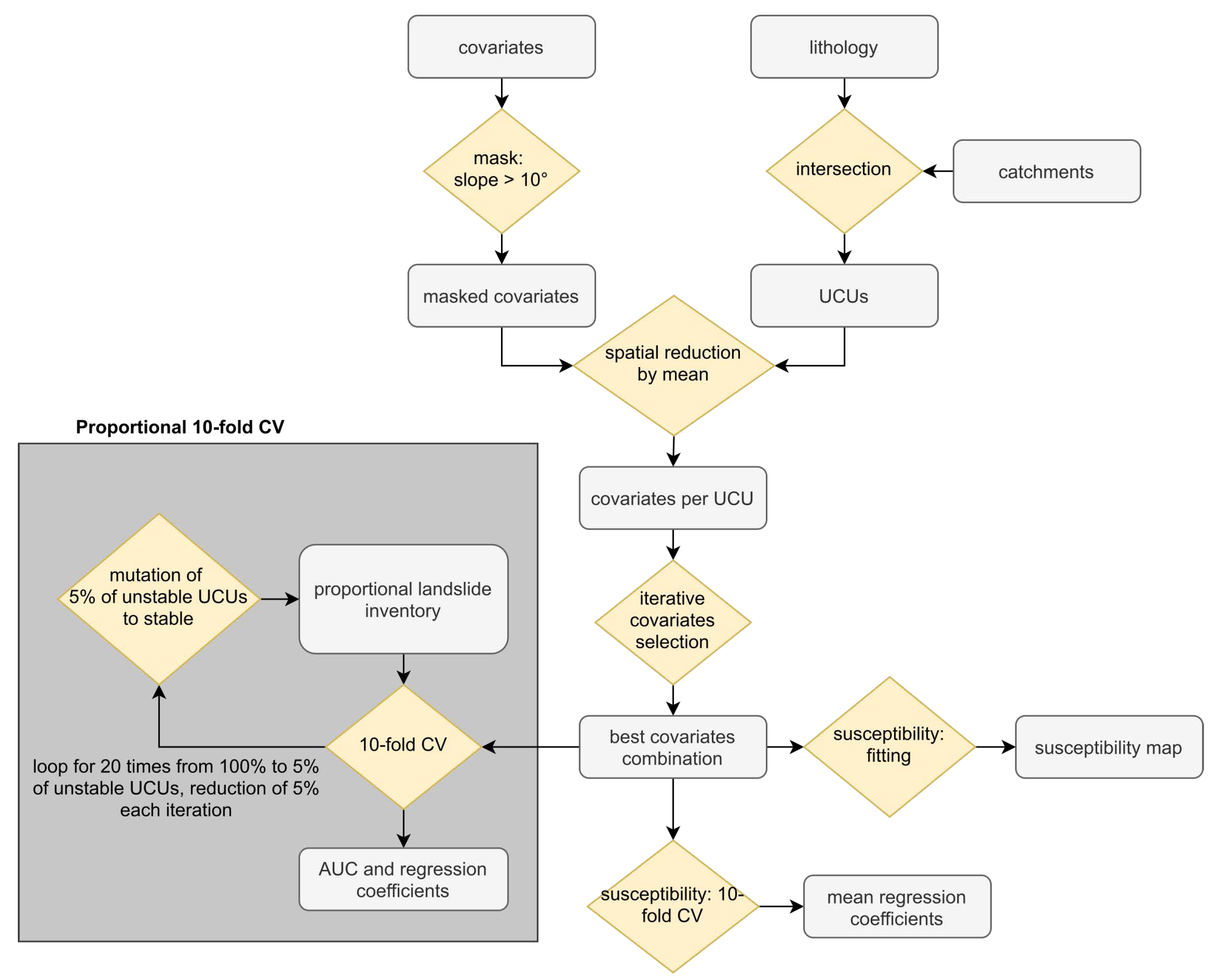
2.4. Modeling Strategy

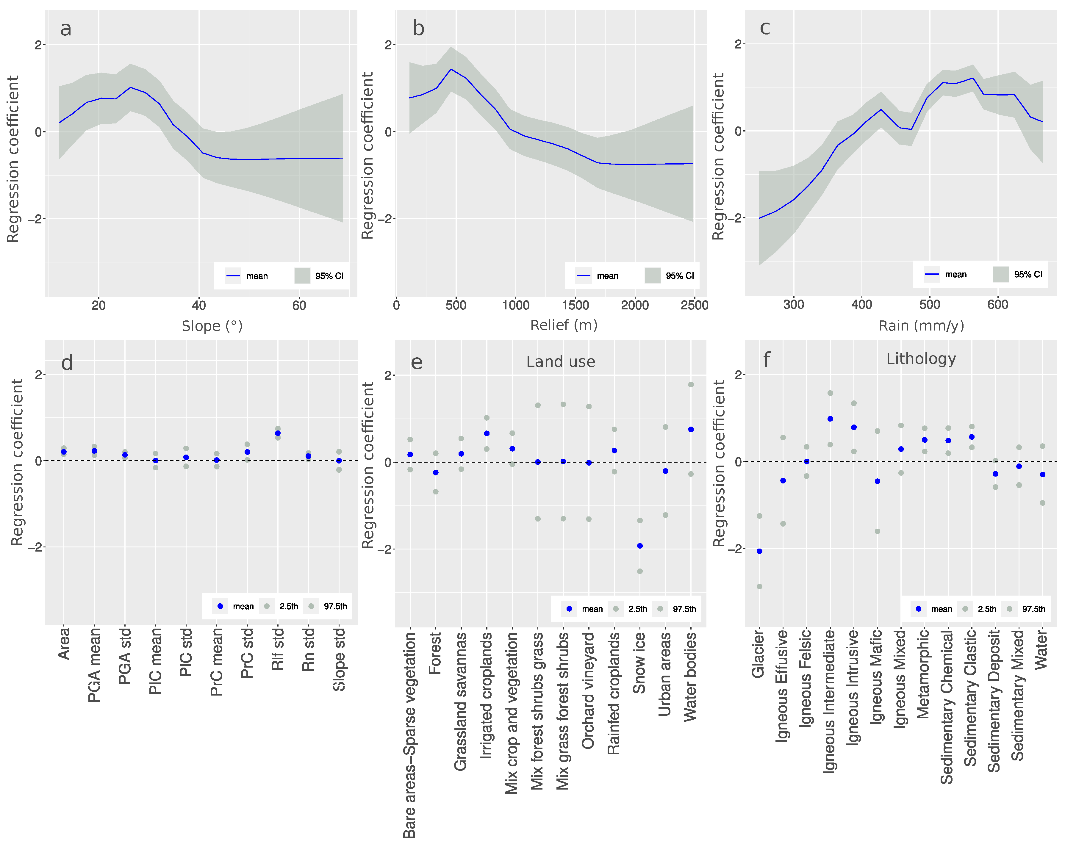
2.4.1. Generalized Additive Model

To estimate the landslide susceptibility of Tajikistan, we chose a Bayesian version of a binomial Generalized Additive Model (GAM) [22,54]. This is being implemented in INLA [55,56].

The binomial GAM we implemented can be denoted as follows:

$$\eta \left(P\right)={\beta }_0+\sum _{j=1}^J{\beta }_j{x}_j+f\left(Litho\right)+f\left(LU\right)+f\left(R{n}_{\mu }\right)+f\left(Slop{e}_{\mu }\right),$$

(1)

where:

• $\eta$ is the logit link;
• P is the probability of landslide occurrence;
• ${\beta }_0$ is the global intercept;
• ${\beta }_j$ are the jth regression coefficients estimated for the xth covariates which we modeled as fixed effects (or linear properties);
• $f\left(Litho\right)$ and $f\left(LU\right)$ are two random effects (non linear properties), which we modeled as independent and identically distributed (iid) covariates. This implies that the regression coefficient associated with each class is estimated independently from the other classes;
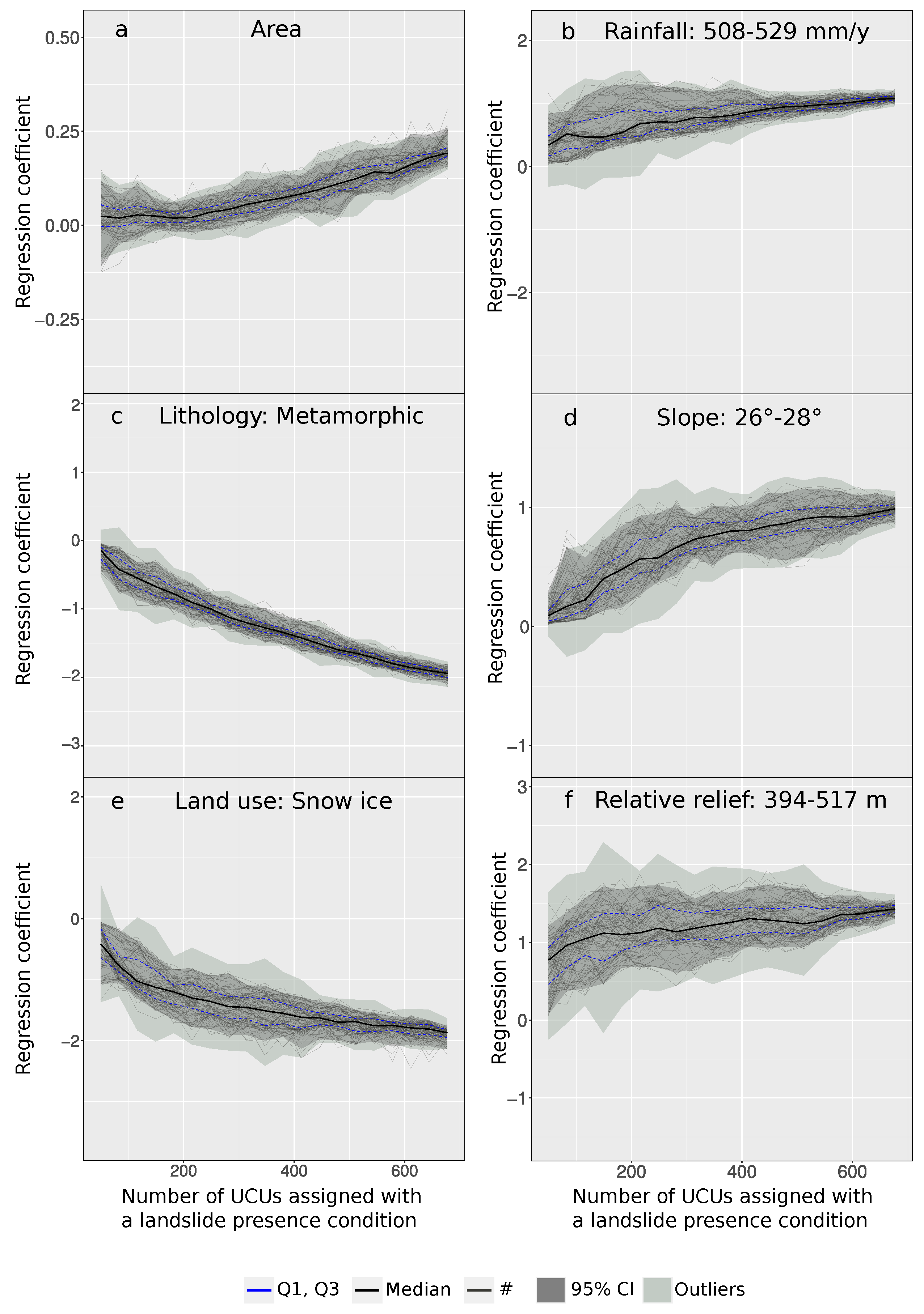
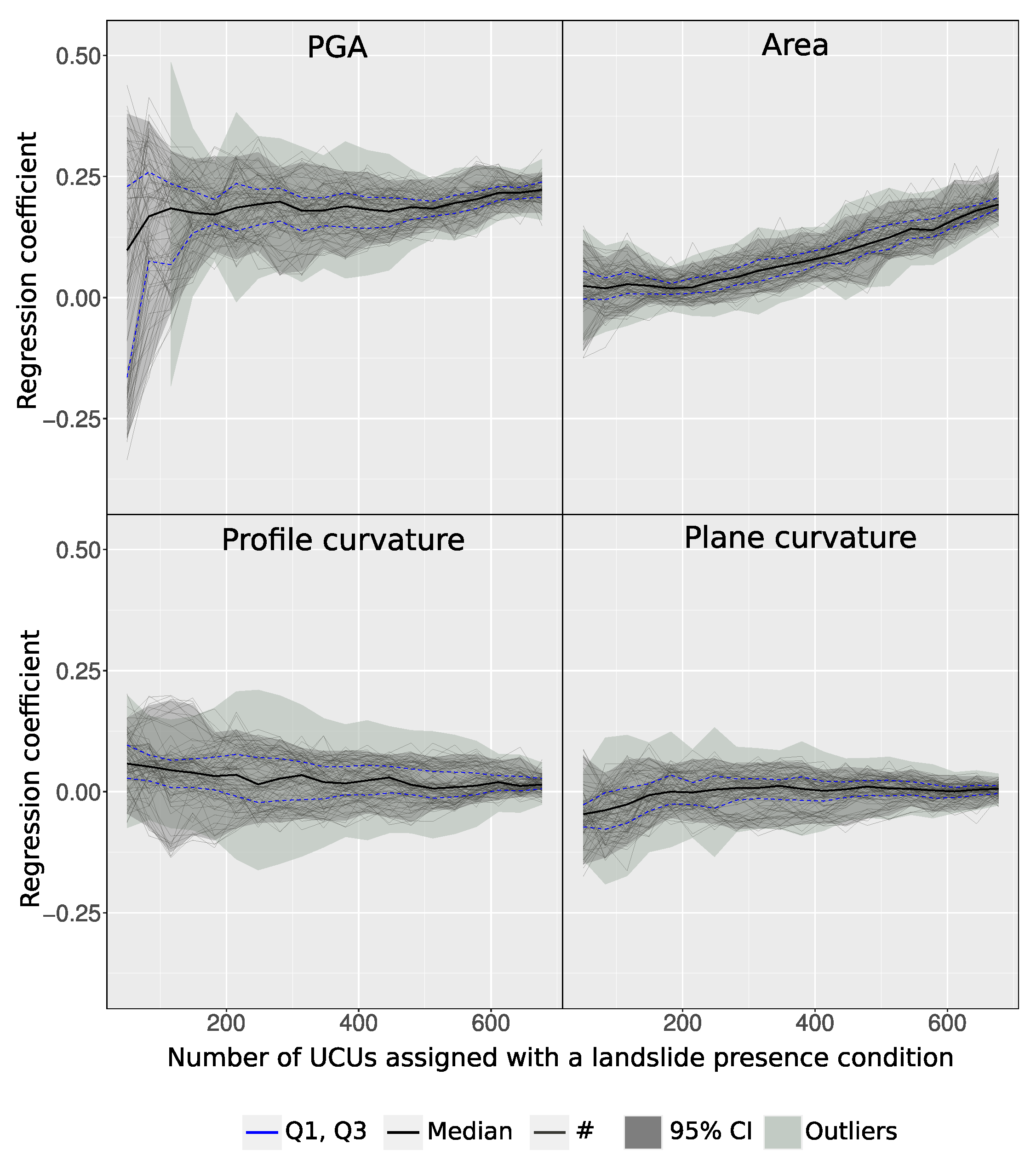
• $f\left(R{n}_{\mu }\right)$ and $f\left(Slop{e}_{\mu }\right)$ are two random effects (non linear properties) that we modeled as random walks of the first order ($rw1$) covariates. This implies that the regression coefficient associated with each class is estimated with an adjacent class dependence. In other words, the coefficient of a single class depends on the coefficient estimated for the class before and after. The use of a random walk allows one to retain the ordinal structure of a covariate that was originally continuous in nature, which we reclassified to obtain a non linear function of the same.

The choice of which variable have to be used linearly or non linearly was tested in a pre-processing step where a bivariate binomial GAM was fitted by using one covariate at a time, with a $rw1$ structure. Then, the covariates that exhibited a nonlinear relation with respect to landslide occurrences have been used accordingly, leaving the others as linear properties.

2.4.2. Performance Assessment

To measure the modeling performance throughout the analyses implemented in this work, we use the Receiver Operating Characteristic (ROC) curves and their Area Under the Curve (AUC), following the performance classification scheme proposed by Hosmer and Lemeshow [57].

Specifically, we tested the performance of the reference susceptibility model by using a standard 10-fold cross-validation. This means that 10 times the 90% of the UCUs is used to calibrate the model and the remaining 10% of the whole data are used to test the prediction skill. Notably, each 10% subset was randomly selected with the constriction to not appear in the subsequent sample, ensuring that each testing dataset was mutually exclusive with the others and each sample maintain the exact proportion between presence/absence UCUs of the original dataset.

For models built by using a grid-cell partition, it is more advisable that the cross-validation subsets are also spatially constrained. When this condition is met, we refer to this procedure as spatial cross-validation (see [58]), and it is of fundamental importance to remove any residual dependence in space from the performance assessment. In our case, being the mapping unit a UCU, which is assumed to be independent from the neighboring ones by definition, we did not use an explicit spatial cross-validation although we stress here that this is of fundamental importance whenever the mapping units finely discretize the study area at hand.

Taking one step back, the idea behind a ROC curve is that the spectrum of susceptibility values can be cut into two parts, turning the continuous probability values into two binary label, one consisting of stable slope conditions and the other of unstable ones. These instances can then be matched with the observed data on mapping units that actually contain at least a landslide or not, allowing one to compute confusion matrices reporting True and False Positives as well as True and False Negatives [59]. A ROC curve is then defined by slicing the susceptibility spectrum via multiple cutoffs, storing the True and False Positives Rates each time.

In this work, not only were the ROC curves used to assess the model performance but we also took inspiration to produce a robust classification of the susceptibility map. The literature is rich of articles where different approaches to classify the susceptibility are used. These span from using a quantile description to more robust statistical criteria with no justification at all (details in [27]). In this study we decided to classify the maps in four susceptibility classes: Very low, low, high, and very high. To select the best four probability cutoffs, we tested a large number of combinations through an optimization algorithm (Genetic Algorithm-based) and extracted the four thresholds that yielded the highest AUC value [60]. This was done both by using a cutoff that best replicates the number of unstable UCUs per probability bin (classical ROC), and by using the cutoff that best replicates the area (with slope > 10°) of unstable UCUs per probability bin (ROC weighted over the UCUs area).

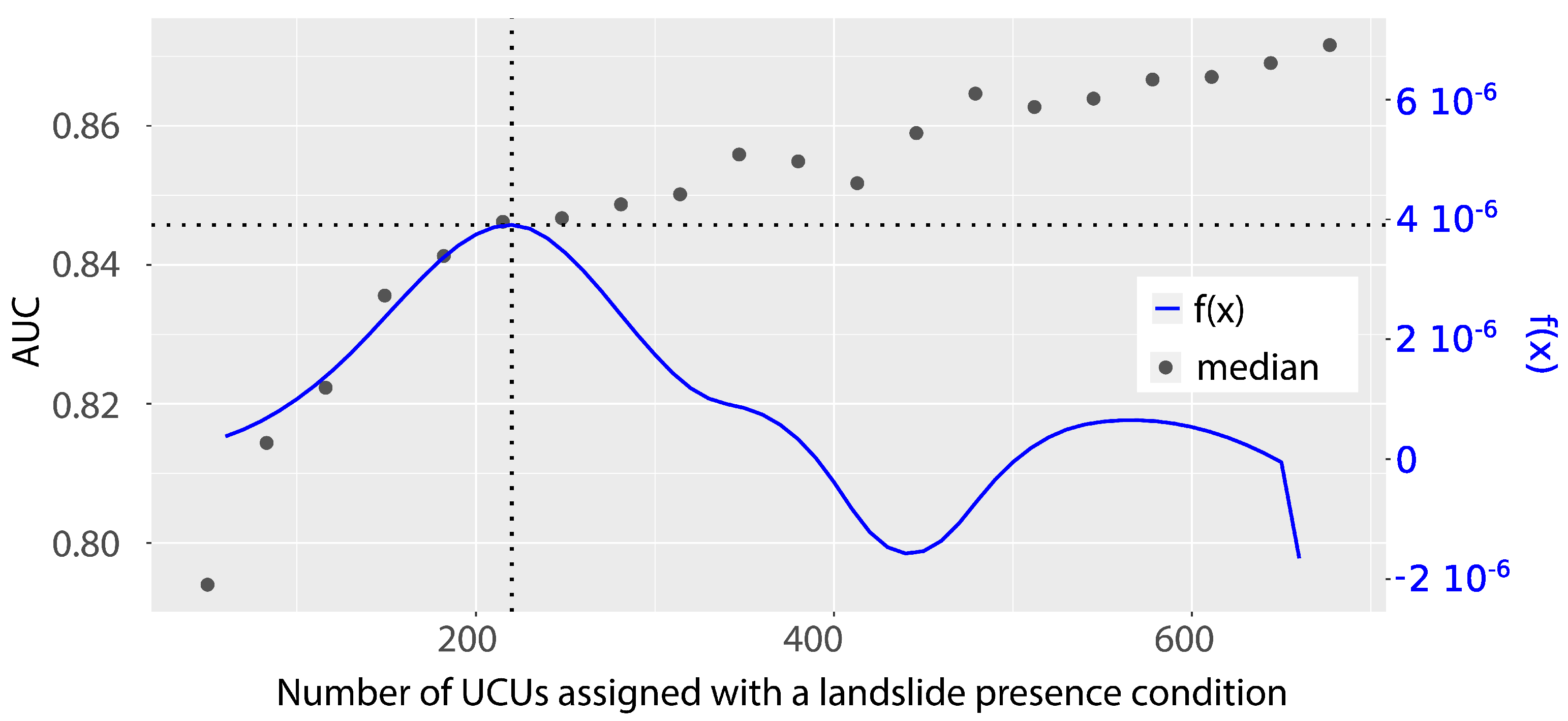
2.4.3. Fitting Different Presence Data Proportions

To investigate the effect of partially-mapped landslides in a data scarce environment, we fitted several binomial GAMs at varying proportions of presence information in the model. Specifically, we used a reference model fitted by using the whole landslide presence/absence information and then, we compared to the reference, a series of models fitted by randomly changing the presence instances into absences. This operation numerically mimics a situation where an actual mapping unit containing a landslide is not properly scanned, thus leading one to miss the landslide occurrence at that location and assigning an absence condition to that UCU. Our random substitution of presences into absences has been gradually run, switching 5% of the total presences at a time, from 0% of the total presence to the 95%. This means that the second run has included 95% of the landslide inventory (5% turned into absences) and the last run with 5% of the inventory. In this manner, each run is linked to the previous by the same landslides sample minus its 5% (as absolute value, the 5% is always relative to the total presences with no switches). Each substitution has been tested with a 10-fold cross-validation. The entire operation has been repeated 10 times for each substitution, creating a routine for which the prediction was tested with respect to the remaining data, which was left unchanged (landslide presences were still presences). In total, 2000 runs has been completed.

As a result of this procedure, we monitored the variation in AUC as the landslide presence information decreased to just 5% of the data we used in the reference model. We also monitored the variation in the regression coefficients estimated for each covariate, being either linearly or nonlinearly used in our model.

A graphical summary of the analytical protocol we proposed is shown in the flow-chart of Figure A1.

3. Results and Discussion

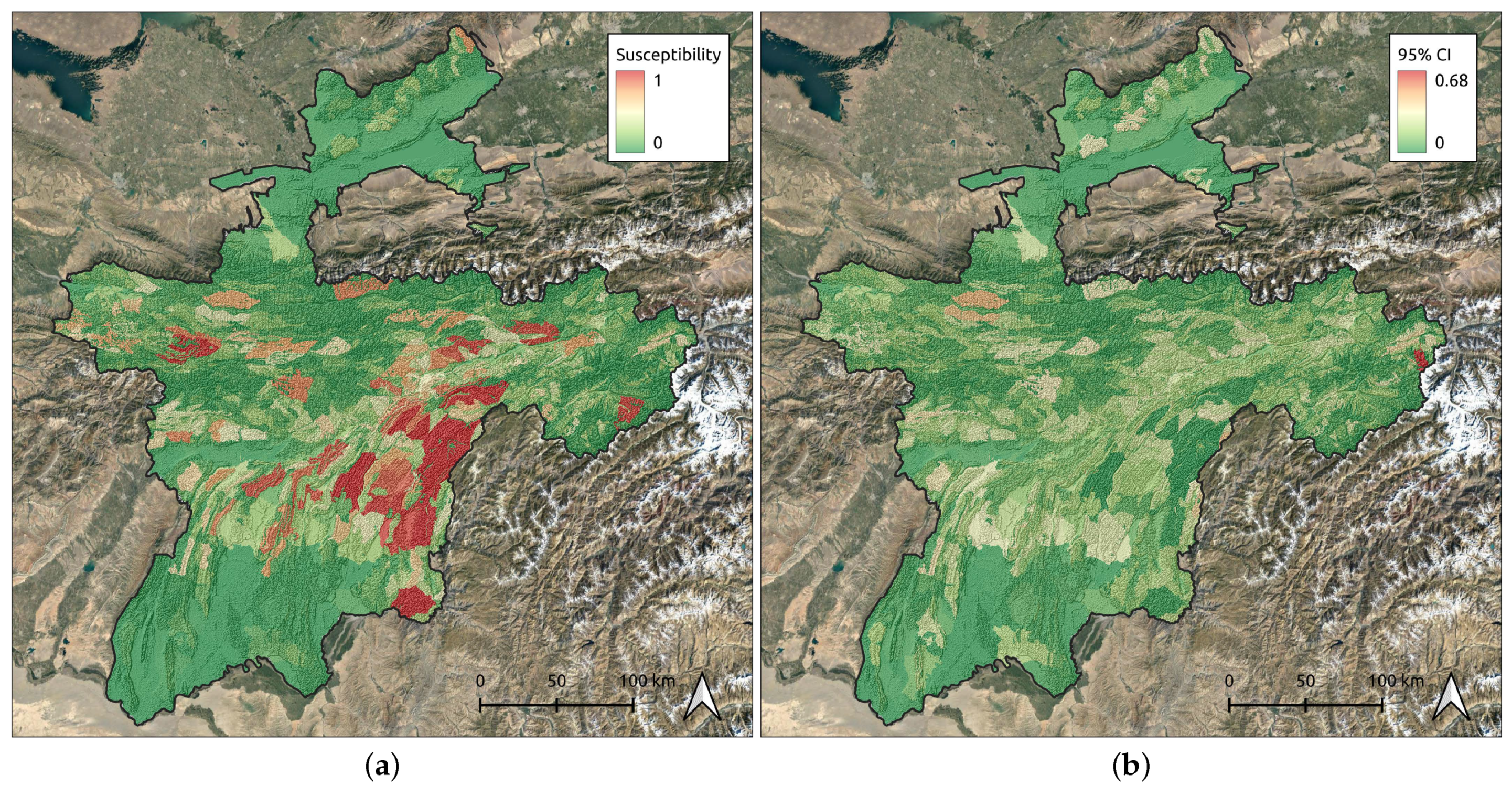
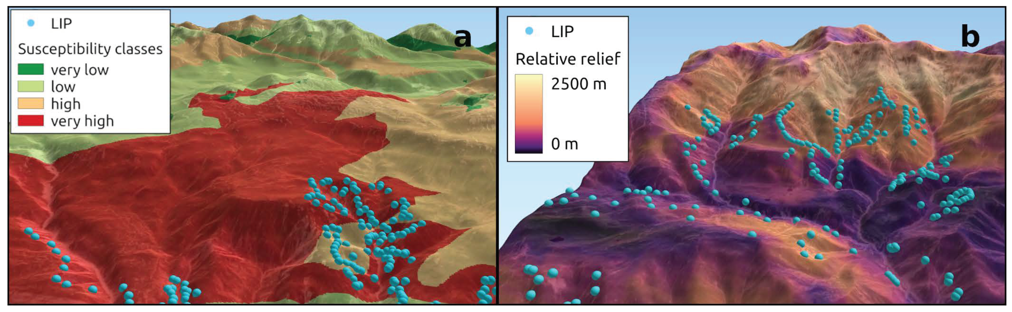
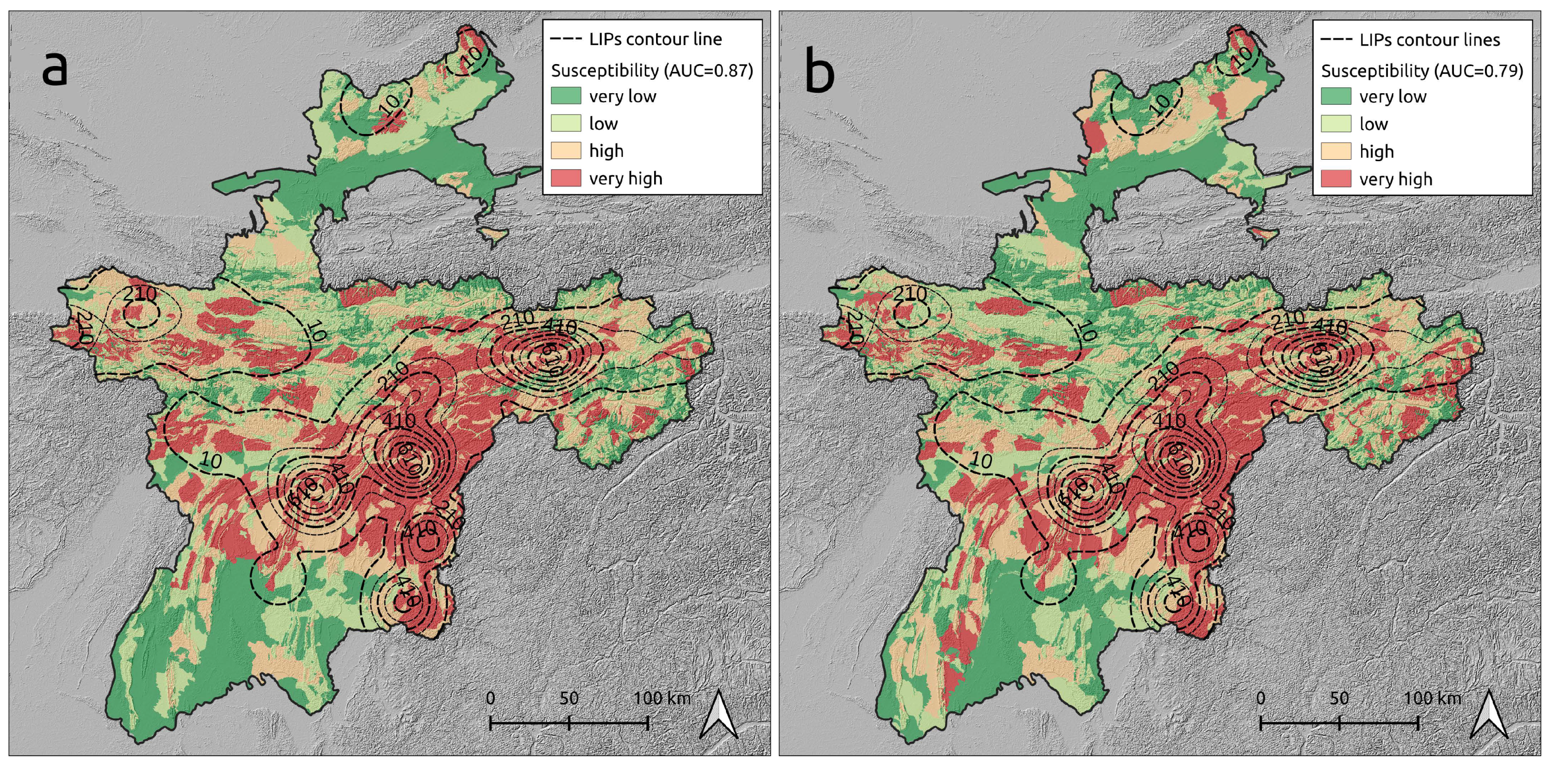
3.1. Reference Susceptibility Model

The first model we tested represents the benchmark for the subsequent analyses. It is trained by fitting a model informed of the total number of unstable UCUs and by featuring all the stable UCUs at the same time. The associated area under the ROC curve (AUC) is 0.88, which is considered an outstanding performance class according to the criteria proposed by Hosmer and Lemeshow [57]. The corresponding susceptibility map (measured in terms of posterior mean and its 95% credible interval) is shown in Figure 4, where we use the continuous spectrum of probability values to plot it in the left panel.

We present each model component in Figure 5. Here the three panels in the first row report the nonlinear effects of the mean slope steepness (Figure 5a), mean relief (Figure 5b), and mean annual precipitation (Figure 5c). The first two appear to share a similar effect: Relatively low steepness and relief values being associated with high regression coefficients whereas the remaining distribution appears to be either not correlated or even negatively correlated to landslide occurrences. As for the rainfall, the pattern appears to be reasonable, with low annual average precipitations being associated with negative regression coefficients, which rapidly increase as the rainfall amount increases.

In Figure 5d, the linear contributions of the UCU area and PGA appear to be significant, increasing the probability of landslide presences per mapping unit. It should be noted, however, that there is only one major earthquake-induced landslide inventory available (for the Khait earthquake in 1949) and that therefore the mapped landslides do not reflect earthquake-triggered events in their majority. Conversely, the plan and profile curvatures were estimated to be not significant and with a posterior mean value around zero. This is related to the selection process of the UCU, which contains often fairly large units with large topographical variations.

The categorical variables, land use (Figure 5e) and lithology (Figure 5f), present a large variation in significance per each category. In detail, land use reveals a significant contribution to increase the probability of landslide presence per UCU with several land use types that have a positive contribution to the presence of landslides. The class with bare or sparse vegetation seems to have less contribution to landslide occurrence that we originally expected. The units with waterbodies have a higher contribution than expected, due to the fact that the slopes around existing hydropower dams have a relatively high landslide density, and the available inventories were more detailed for the areas surrounding hydropower projects. The areas covered by snow and ice decrease the probability of landslide presence per mapping unit. This can also be explained by the difficulty of mapping landslides in these high mountain terrains, where many of the available satellite images have a snow cover, thus leading to a possible (or not) under representation of landslides mapped in these areas.

As regard the role of lithological classes, a large number was estimated to be significant and most were recognized to positively contribute to the susceptibility estimates. These correspond to: Igneous intermediate, igneous intrusive, metamorphic, sedimentary chemical, and sedimentary clastic rocks. Among these, the highest mean regression coefficient is estimated for an igneous intermediate substratum. This could imply that the detrital mantle and soil draping over this bedrock type can be rich in clay as this mineral is the natural product of the long-term weathering effect on igneous rocks [61]. In turn, clays could be responsible for shallow landslides [62] as they are subject to shrink and swell processes at varying soil moisture conditions. Similar to the land use class, the posterior mean value of glaciers in the lithology map is highly negative.

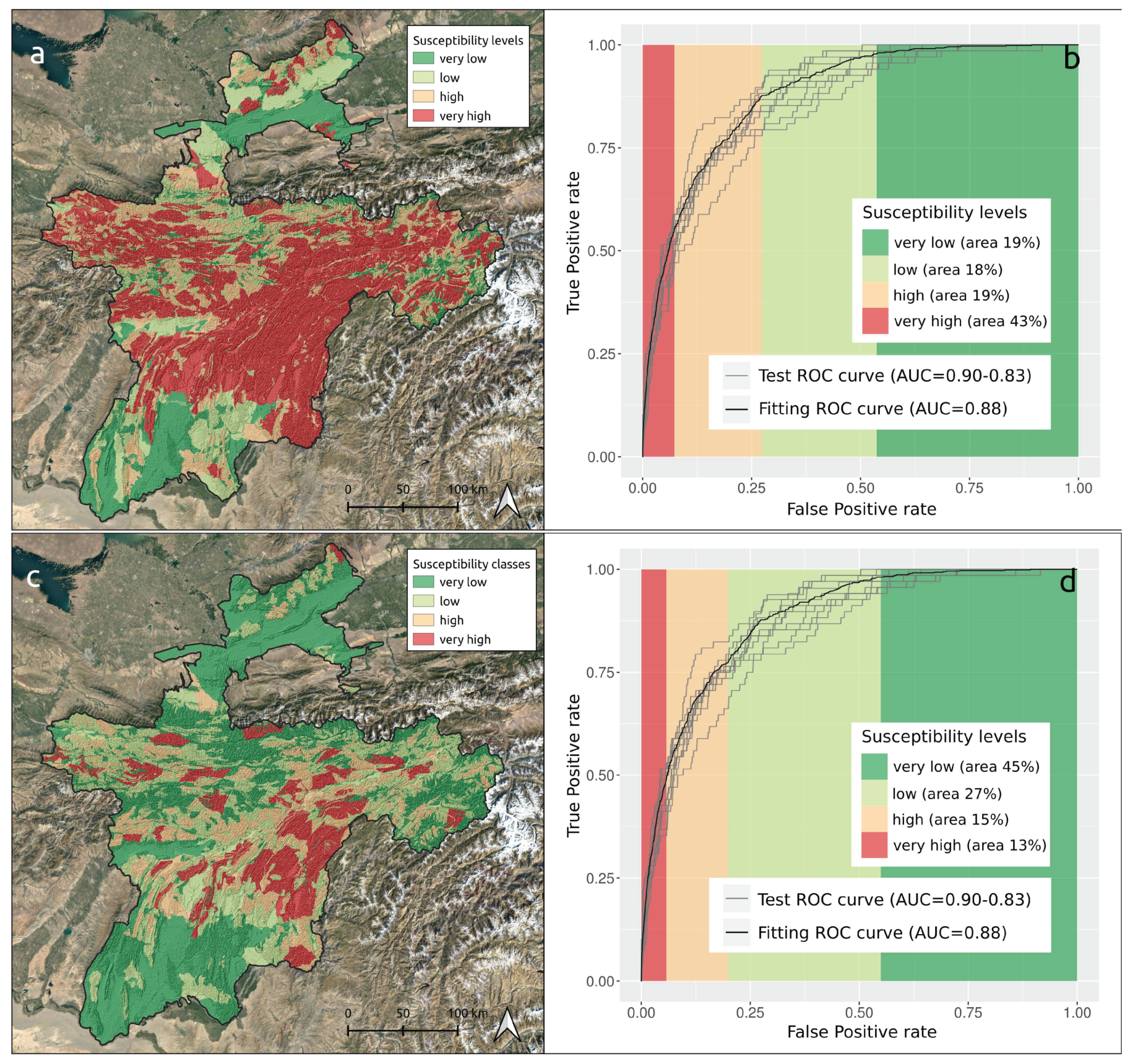
3.2. First set of Cross-Validations

From the 10-fold cross-validation, we extracted the posterior mean to compute the AUC for each replicate. The average AUC out of the 10 calculations is 0.87, and a variability measured with a two-times standard deviation is equal to 0.02. The continuous spectrum of probability which composes the susceptibility map resulting from the first set of traditional cross-validation runs has been classified using two different criteria. The maps are shown in Figure 6a,c. We classified the probabilities using the SZ-plugin developed by Titti et al. [60]. The upper map (Figure 6a) is classified by selecting the edges of each class equal to the cutoffs that maximize the AUC of the segmented ROC curve, which means to maximize the number of unstable UCUs per probability bin. Therefore, being the UCUs irregular spatial objects, the map appears dominated by very high susceptibility conditions. Conversely, the bottom map is generated by cutoffs that maximize the area (with slope > 10°) of unstable UCUs per probability bin (the relative ROC curve is weighted over the area extension). Here the maps appear much more realistic and similar to the benchmark presented in Figure 4 with the main difference being expressed in the extension of the red area, which covers 43,058 km${}^2$ (43% of total area, see Figure 6b) in the first classification and 10,012 km${}^2$ (13% of total area, see Figure 6d) in the second classification.

Figure 7a provides two interesting perspectives on the analyses we have run. It demonstrates that the susceptibility pattern (taken from Figure 6c) closely reproduce the spatial distribution of landslides at the scale of the UCUs. Figure 7b complements this information by highlighting that the highest susceptible zones are not necessarily those with the highest relief, but with the most susceptible lithologies, in combination with the highest levels of rainfall and earthquake acceleration. The relatively lower susceptibility of the high elevation, snow- and ice-covered regions is due to the limited availability of inventories for these areas, and may not reflect the actual situation, or the possible future situation, where climate change will contribute to decreasing glacial coverage.

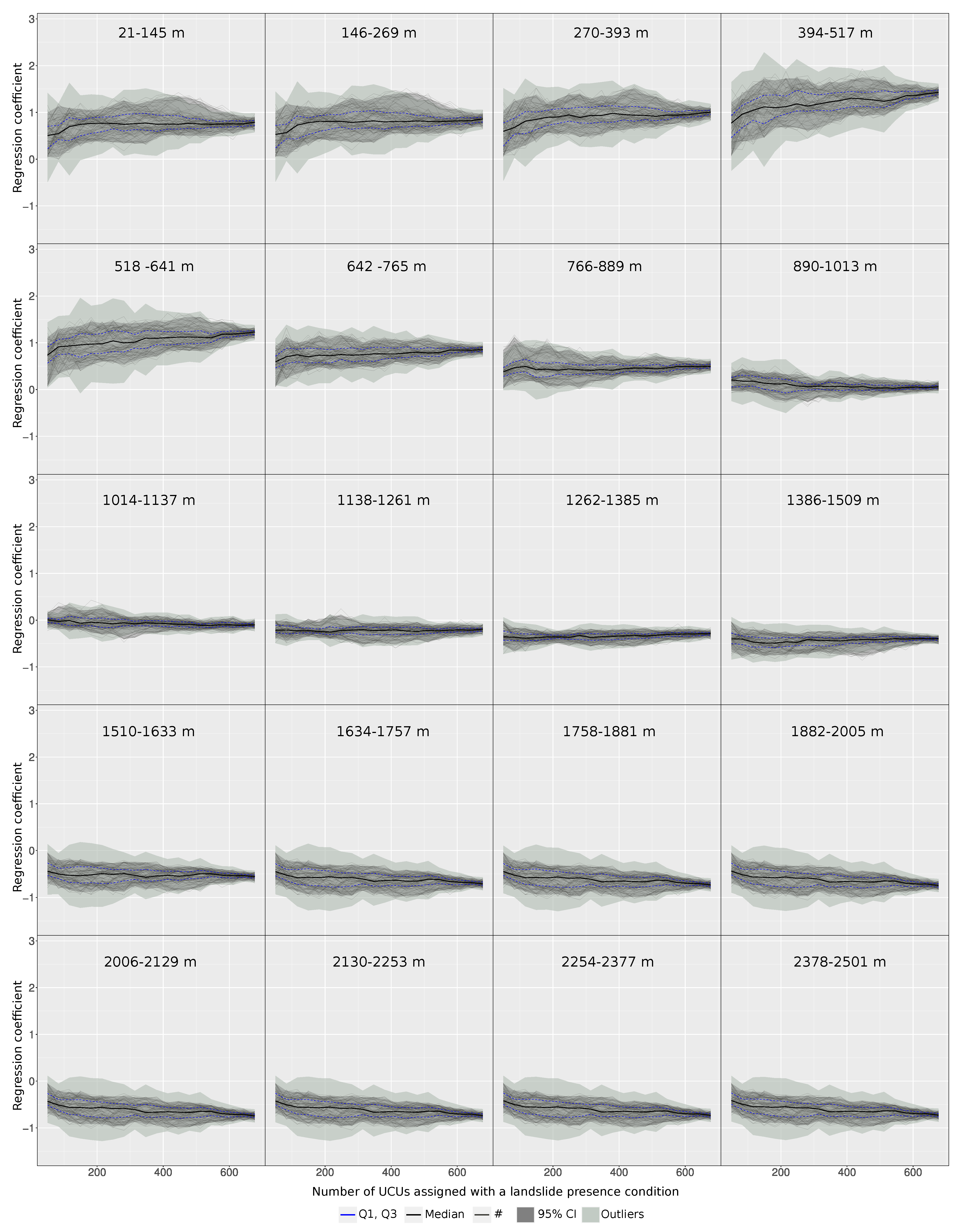
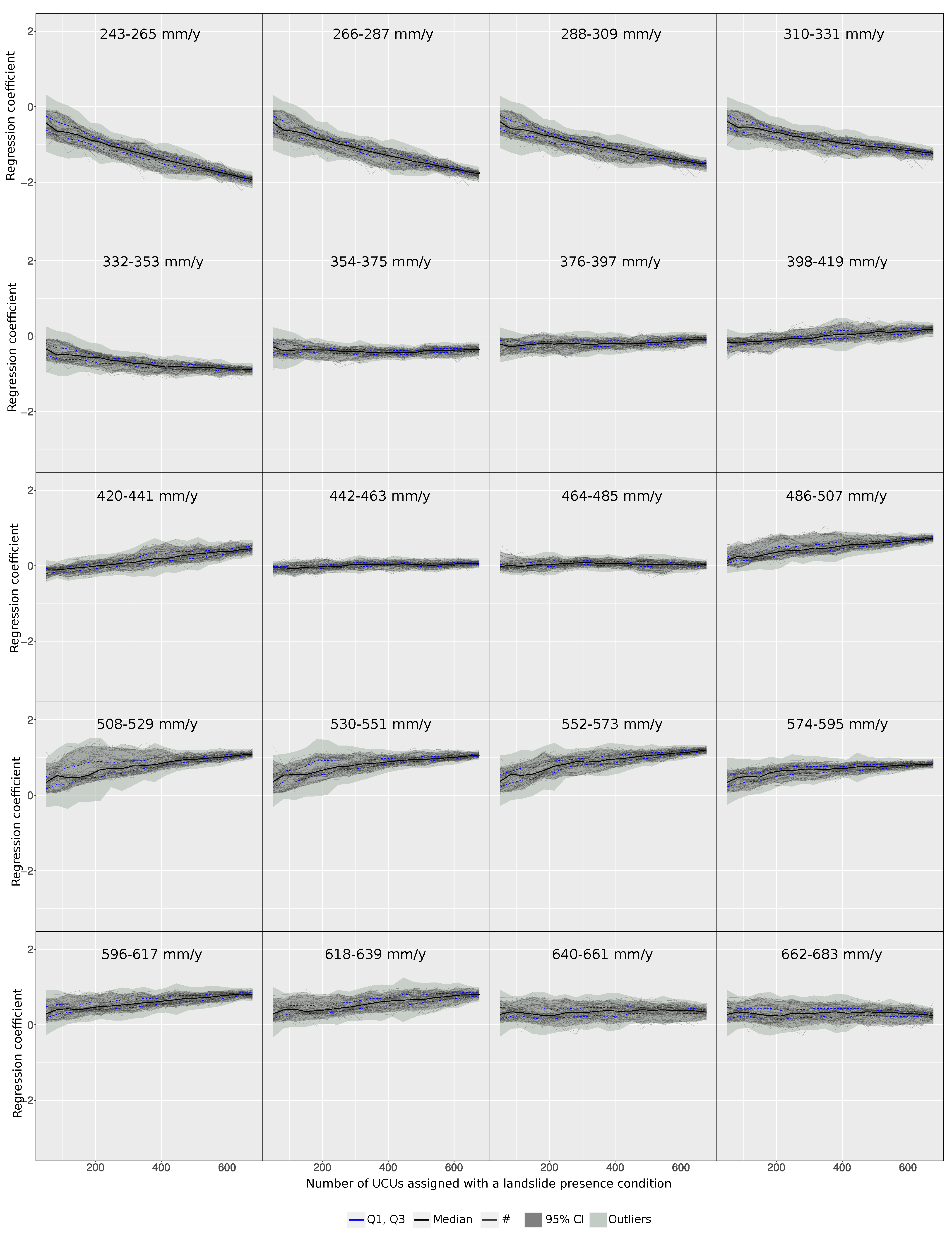
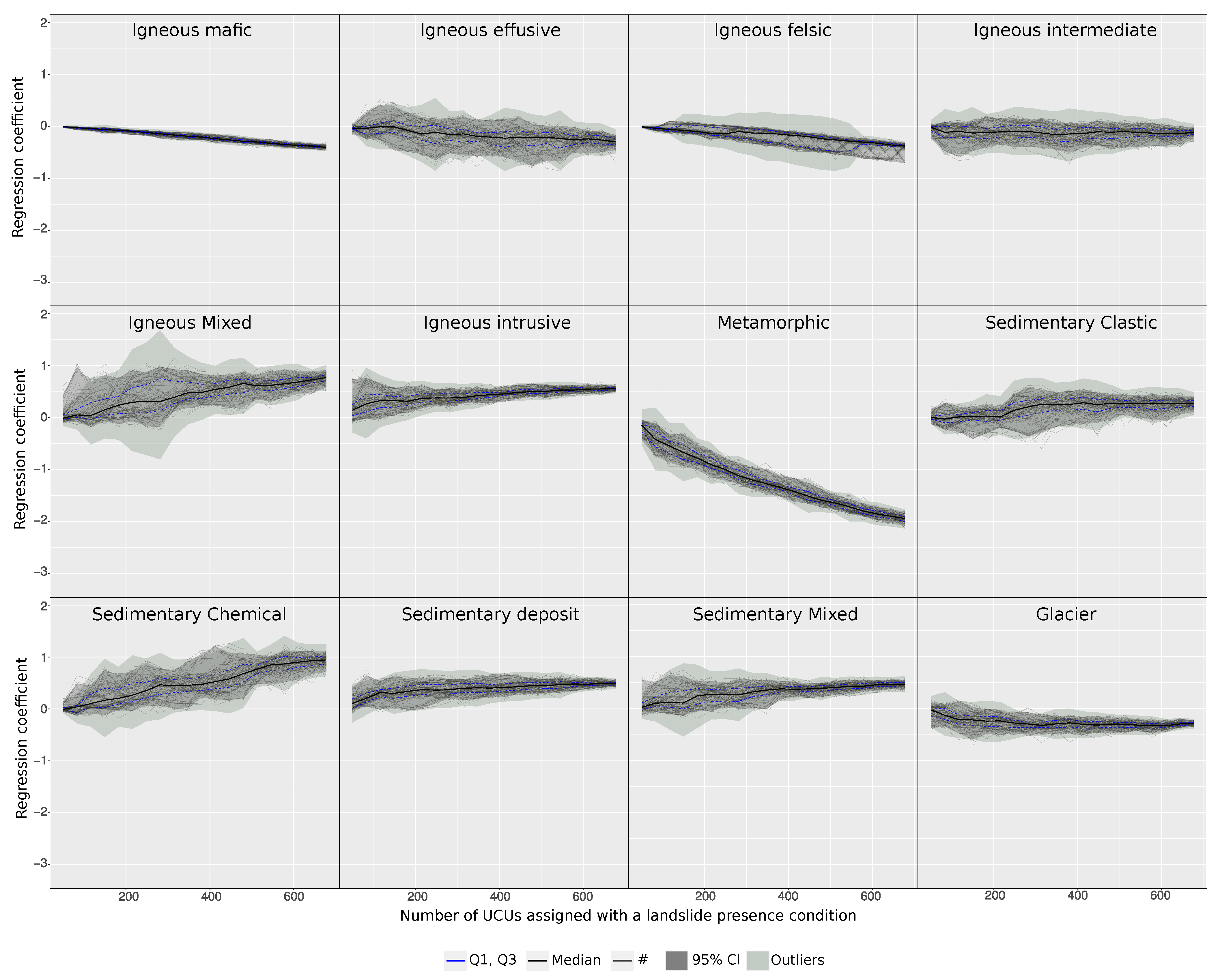
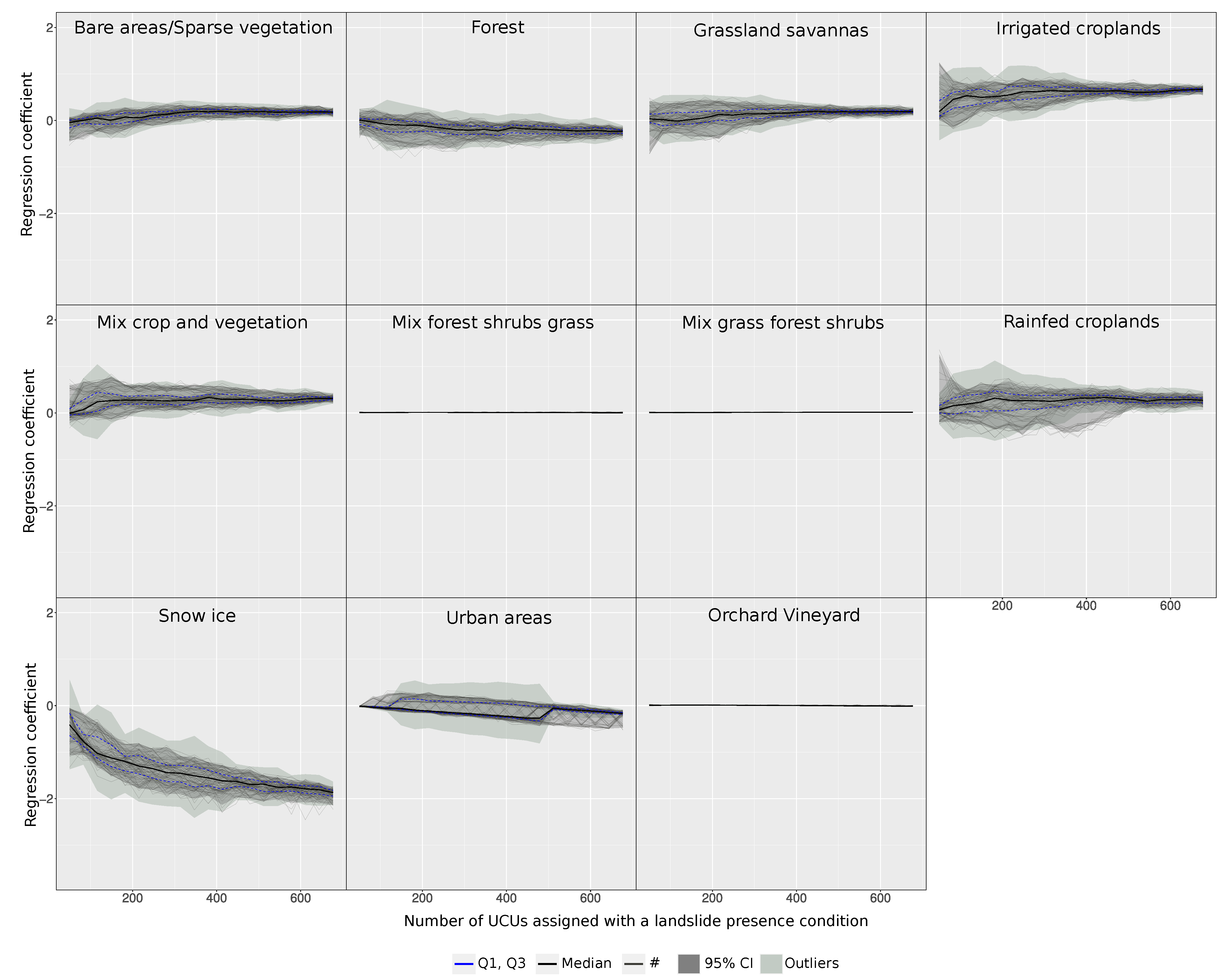
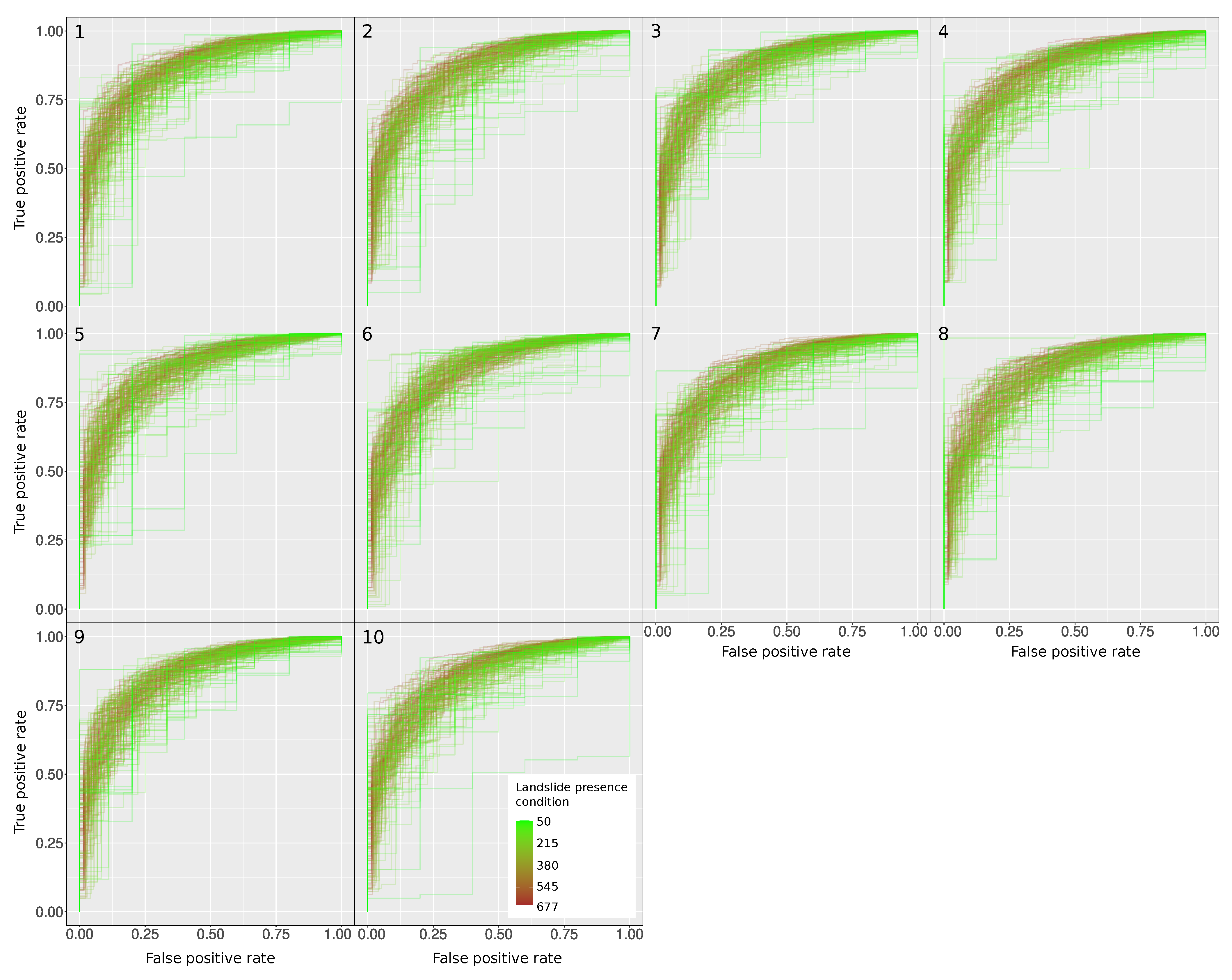
3.3. Sensitivity Analyses at Varying Landslide Presence

In this section, we evaluate the results from the varying proportions of landslide presences per UCU, and compare them with the reference susceptibility model presented in Section 3.1. Figure 8 reports the AUC values obtained for each cross-validation routine from an initial landslide presence sample of 50 UCUs (5% of the reference inventory) up to 677 UCUs (100% of the reference inventory). Surprisingly, the corresponding difference in performance is not as evident as we initially assumed. In fact, just 5% of the reference inventory is enough to reach a median AUC of approximately 0.79. Conversely, 100% of the reference inventory produced a median AUC of 0.87. The latter corresponds to an outstanding performance according to the classification scheme proposed by Hosmer and Lemeshow [57], being clearly preferable to a 0.79 (all the ROC curves are visible in Figure A8). However, in reality the difference in the time and efforts required to map less than one hundred or several hundreds of mapping units with landslides is very large. Thus, specifically for Tajikistan, such a result inevitably raises the question why this happens and whether it is worth to invest resources in mapping landslides when fewer mass movements already produce suitable predictive performances.

Comparing the classified susceptibility maps assessed as the median of the 10 runs with 100% (Figure 9a) and 5% (Figure 9b) of total landslide inventory, it is evident how much the latter is less reliable than the former. In particular, this is clearly visible in the southern and northern part of Tajikistan where, on the contrary to the map in Figure 6c and to the map in Figure 9a, in the susceptibility map modeled with the 5% of total landslides available (Figure 9b), the classes ‘high’ and ‘very high’ cover a larger area.

To investigate this result further, we carefully checked the area and recognized, as also shown in Figure 5, that landslides generally occur in very similar morphometric situations in Tajikistan. At a medium slope and medium relative relief values they are abundant, whereas they tend not to be represented where snow and ice cover the landscape (mainly at high relative relief values). This is interesting because we cannot know whether this effect is real. In fact, snow cover tend to hide landslides or make it impossible to separate a landslide from other active processes, such as snow avalanches, that dominate a high portion of relief. Therefore, with the same probability, landslides may actually be considered absent and present.

Landslides tend to cluster in the wettest portion of the Tajikistan territory. As for the signal captured by categorical properties, many lithologies are quite susceptible to landslides, and contribute more to susceptibility than land use types. The lithological units were grouped into rather broad classes, and therefore the combination of covariates that results in high susceptibility can be characterized by using a relatively small number of UCUs. However, the high AUC values could also be related to the large dimension of the UCUs. Lima et al. [63] states that a “too detailed representation of the terrain may be detrimental in the presence of inaccurate landslide data”. In our case, since the UCUs are rather large terrain units, this could attenuate the effect of the incompleteness we induced by decreasing the number of presences.

We justify the relatively similar predictive performance through the considerations provided above. However, to support them numerically we checked their validity by examining the variations in the estimated regression coefficients as the proportion of presences changed. For conciseness, a brief overview of this procedure is provided in the main text through Figure 10. There we exemplify for the reader the variation of the regression coefficients related to six covariates (one fixed effect, and five classes extracted from five respective random effects), plotted as the information on landslide presence data increases. In Appendix A, we report the variation of the regression coefficients for all the model components estimated to be significant. Specifically, Figure A2 shows the variation for the four fixed effects. The PGA and the two curvatures essentially exhibit the same regression coefficient irrespective of the number of presence conditions in the dataset and among each of the bootstrap replicates. Conversely, the UCU area over 10° of the slope becomes more positive as the proportion of presences increases.

To provide an overview of what happens with a covariate used in a non linear fashion, we report the effects estimated for each of the mean slope steepness classes, mean relative relief classes, and mean annual rainfall classes. The behavior of the slope steepness is shown in Figure A3 where the variations as the number of presence instances in the dataset appear to be stronger than for the linear covariates mentioned before. Specifically, as the number of landslide presences increase, the mean steepness classes 20°–22°, 23°–25°, and 26°–28° are estimated with an increasingly positive contribution to the susceptibility. This trend appears to be interrupted from the class 29°–31° and to invert itself for the classes from 38° to 69° where the regression coefficients become increasingly negative as the proportion of landslide presences increases.

Mean relative relief has been subdivided into 20 classes (Figure A4). The first 7 classes show positive regression coefficients, whereas the others became increasingly negative as the relative relief increases. As the proportion of landslide presences change in each relief class, the regression coefficients remain constant.

On the contrary of the sinusoidal behavior of the slope covariate, precipitation presents a discontinuous trend between the minimum and maximum annual rainfall recorded in 10 years in Tajikistan (Figure A5). In particular, increasing the number of landslides in sample, it contributes negatively to susceptibility from 243 mm/y to about 375 mm/y where the trend inverts itself, the regression coefficients became increasingly positive as the proportion of landslide presences increases from 486 mm/y. The classes between 375 mm/y and 486 mm/y do not significantly contribute to estimate the susceptibility.

The situation for the categorical properties is also quite interesting (see Figure A6 and Figure A7). Metamorphic lithotypes (Figure A6) exhibited the largest variation as the proportion of landslide presences increases. Specifically, they increasingly contribute in a negative manner to the susceptibility model. Other examples exist where the situation is the opposite albeit with a less striking pattern, these being mixed igneous rocks and chemical sedimentary materials.

The land use classes (Figure A7) show a much more stable response to the landslide presence content in the dataset and across cross-validation replicates. The only exception consists of the snow/ice class, which contributes to decreasing the estimated probability of landslide occurrences per UCU.

Notably, across all these plots not a single example exists where we monitored an inversion of the regression coefficient sign as the proportion of landslides increased. This is a fundamental point which justifies the fact that performance-wise, no extreme changes can be observed at varying presence conditions in the training dataset.

To answer the main question of this paper, starting from a complete landslide inventory, we mapped the landslide susceptibility of west Tajikistan and repeated the same analytical protocol, gradually reducing the amount of landslides presence condition of each UCU, labeling them as stable. As a result, we induced systematic incompleteness and associated biases [63] in the the analyses. We did this in the hope of finding a numerical threshold above which the susceptibility map is not sensitive to the addition of new unstable mapping units. However, the AUC distribution plotted in Figure 8 was quite smooth. Although, the transition from median AUC values of 0.79 to 0.87 is an interesting trend to monitor, recognizing a single number of unstable UCUs that separates two different predictive behaviors could not be found.

To further deepen our observation, we opted to calculate the rate at which the median AUC shown in Figure 8 varies from small to large samples of unstable UCUs passed to the model. This is shown in Figure 11 where the rate of change between the subsequent AUC median has been measured with a function $f\left(x\right)$, explained as follows:

$$f\left(x\right)=\Delta g{\left(x\right)}_k^{\prime }-\Delta g{\left(x\right)}_{k-1}^{\prime }$$

(2)

where, $g\left(x\right)$ is the median function, $\Delta g{\left(x\right)}^{\prime }$ is the gap between two consecutive first order derivatives of $g\left(x\right)$ in sliding windows, and $f\left(x\right)$ evaluates how fast the curve trend changes by the difference between the gaps $\Delta g{\left(x\right)}^{\prime }$ of the sliding windows and the previous. Interestingly, the maximum of $f\left(x\right)$ corresponds to 220 UCUs assigned with a presence condition (32% of unstable UCUs and 1.5% of the total UCUs). After this, the model does not significantly improve and therefore, we consider this value as the minimum amount of presence condition required for this study area.

This framework raised the question of when shall the inventory be considered complete and what would have been the implications if we would have stopped mapping earlier than the deadline we set. All the analyses we then performed have been voted to address this issue. A series of sensitivity checks have been tested at decreasing numbers of unstable UCUs.

This observation is much more interesting than the one based on Figure 8 and it does answer the main question posed at the beginning. However, this result may be site-specific and not generalizable to other study sites or to other kinds of mapping units.

4. Conclusions

This research was part of a large international project for which a landslide susceptibility assessment was required for landscapes intersected by the new silk road. The first limitation we found was to access landslide inventories in countries with scarce data availability, among which is Tajikistan. As a result, we mapped landslides under the assumption that we could not map them all and that at a certain point, we should have stopped and considered our inventory suitable for susceptibility modeling.

This framework raised the question when the landslide inventory can be considered complete enough to serve as a basis for susceptibility modeling and what would have been the implications if we would have stopped mapping earlier than the deadline we set. All the analyses we performed were aimed to address this issue, including sensitivity checks tested at decreasing numbers of unstable UCUs. The susceptibility patterns and associated performances appeared quite robust, with relatively small differences when using a small or a large sample of unstable UCUs. This may be due to the relatively coarse spatial partition we adopted, and the use of the UCUs, which were defined as the intersection between catchments and geological units.

The susceptibility analysis measures the propensity of the territory to generate landslides, from the presence/absence information associated to the mapping units and from the selected covariates. The small variations we found may imply that UCUs are already sufficient to capture the landslide distribution even with a relatively small sample of landslides, and that UCUs that are unstable share very specific characteristics. In fact, the difference in AUC between a median model yielding 0.79 and a median model yielding a 0.87 approximately corresponds to just 80 km${}^2$, for the very high susceptible class in quartile classification. Therefore, from a pure performance perspective, it seems that it could have been convenient to stop mapping long before the deadline we set for ourselves. However, merely looking at the absolute performance would be a mistake. In particular, the spatial distribution of the probability with an AUC of 0.79 shows high and very high levels of susceptibility in areas where we expected stable conditions.

Therefore, we further investigated the best compromise in between the two extremes. This is shown in Figure 11 where we measured the rate of variations in AUC as the unstable sample increased. There, the largest variation coincides with 220 unstable UCUs, after which the improvement rate of the susceptibility significantly drops.

One of the limitations in the generalization of the results we obtained may be due to the mapping unit we chose. In fact, coarser mapping units are less sensitive to variations in the number and distribution of landslides. Conversely, smaller mapping units would likely capture the variations induced by our modeling strategy at varying landslide proportions. This in turn may have led to variations in model performance and covariate effects. We are currently testing the same analytical protocol on the basis of a slope unit-based partition to monitor whether the choice of finer mapping units may yield to slightly different conclusions.

All these considerations could still be very local and not relevant to any landslide susceptibility studies outside Tajikistan. However, we believe the protocol developed is a very interesting tool to investigate a problem that is heavily underestimated in the literature. We envision future development to measure whether the spatial incompleteness we tested here can be extended to its spatio-temporal counterpart.

To promote reproducible and repeatable analyses and to stimulate further research on this topic, we have shared the R codes at this repository https://github.com/giactitti/GAM-Tajikistan, accessed on 8 November 2021.

References

1. Bout, B.; Lombardo, L.; van Westen, C.; Jetten, V. Integration of two-phase solid fluid equations in a catchment model for flashfloods, debris flows and shallow slope failures. Environ. Model. Softw. 2018, 105, 1–16. [Google Scholar] [CrossRef]
2. Van Den Bout, B.; Lombardo, L.; Chiyang, M.; van Westen, C.; Jetten, V. Physically-based catchment-scale prediction of slope failure volume and geometry. Eng. Geol. 2021, 284, 105942. [Google Scholar] [CrossRef]
3. Carrara, A.; Cardinali, M.; Guzzetti, F.; Reichenbach, P. GIS technology in mapping landslide hazard. In Geographical Information Systems in Assessing Natural Hazards; Springer: Dordrecht, The Netherland, 1995; pp. 135–175. [Google Scholar]
4. Guzzetti, F.; Reichenbach, P.; Ardizzone, F.; Cardinali, M.; Galli, M. Estimating the quality of landslide susceptibility models. Geomorphology 2006, 81, 166–184. [Google Scholar] [CrossRef]
5. Heckmann, T.; Gegg, K.; Gegg, A.; Becht, M. Sample size matters: Investigating the effect of sample size on a logistic regression susceptibility model for debris flows. Nat. Hazards Earth Syst. Sci. 2014, 14, 259–278. [Google Scholar] [CrossRef] [Green Version]
6. Frattini, P.; Crosta, G.; Carrara, A. Techniques for evaluating the performance of landslide susceptibility models. Eng. Geol. 2010, 111, 62–72. [Google Scholar] [CrossRef]
7. Van Den Eeckhaut, M.; Vanwalleghem, T.; Poesen, J.; Govers, G.; Verstraeten, G.; Vandekerckhove, L. Prediction of landslide susceptibility using rare events logistic regression: A case-study in the Flemish Ardennes (Belgium). Geomorphology 2006, 76, 392–410. [Google Scholar] [CrossRef]
8. Petschko, H.; Brenning, A.; Bell, R.; Goetz, J.; Glade, T. Assessing the quality of landslide susceptibility maps—case study Lower Austria. Nat. Hazards Earth Syst. Sci. 2014, 14, 95–118. [Google Scholar] [CrossRef] [Green Version]
9. Conoscenti, C.; Rotigliano, E.; Cama, M.; Caraballo-Arias, N.A.; Lombardo, L.; Agnesi, V. Exploring the effect of absence selection on landslide susceptibility models: A case study in Sicily, Italy. Geomorphology 2016, 261, 222–235. [Google Scholar] [CrossRef]
10. Lombardo, L.; Mai, P.M. Presenting logistic regression-based landslide susceptibility results. Eng. Geol. 2018, 244, 14–24. [Google Scholar] [CrossRef]
11. Steger, S.; Brenning, A.; Bell, R.; Glade, T. The influence of systematically incomplete shallow landslide inventories on statistical susceptibility models and suggestions for improvements. Landslides 2017, 14, 1767–1781. [Google Scholar] [CrossRef] [Green Version]
12. Steger, S.; Brenning, A.; Bell, R.; Glade, T. The propagation of inventory-based positional errors into statistical landslide susceptibility models. Nat. Hazards Earth Syst. Sci. 2016, 16, 2729–2745. [Google Scholar] [CrossRef] [Green Version]
13. Lin, Q.; Lima, P.; Steger, S.; Glade, T.; Jiang, T.; Zhang, J.; Liu, T.; Wang, Y. National-scale data-driven rainfall induced landslide susceptibility mapping for China by accounting for incomplete landslide data. Geosci. Front. 2021, 12, 101248. [Google Scholar] [CrossRef]
14. Steger, S.; Mair, V.; Kofler, C.; Pittore, M.; Zebisch, M.; Schneiderbauer, S. Correlation does not imply geomorphic causation in data-driven landslide susceptibility modelling–Benefits of exploring landslide data collection effects. Sci. Total Environ. 2021, 776, 145935. [Google Scholar] [CrossRef]
15. Jacobs, L.; Dewitte, O.; Poesen, J.; Delvaux, D.; Thiery, W.; Kervyn, M. The Rwenzori Mountains, a landslide-prone region? Landslides 2016, 13, 519–536. [Google Scholar] [CrossRef] [Green Version]
16. Jacobs, L.; Dewitte, O.; Poesen, J.; Maes, J.; Mertens, K.; Sekajugo, J.; Kervyn, M. Landslide characteristics and spatial distribution in the Rwenzori Mountains, Uganda. J. Afr. Earth Sci. 2017, 134, 917–930. [Google Scholar] [CrossRef]
17. Jacobs, L.; Dewitte, O.; Poesen, J.; Sekajugo, J.; Nobile, A.; Rossi, M.; Thiery, W.; Kervyn, M. Field-based landslide susceptibility assessment in a data-scarce environment: The populated areas of the Rwenzori Mountains. Nat. Hazards Earth Syst. Sci. 2018, 18, 105–124. [Google Scholar] [CrossRef] [Green Version]
18. Dewitte, O.; Dille, A.; Depicker, A.; Kubwimana, D.; Mateso, J.C.M.; Bibentyo, T.M.; Uwihirwe, J.; Monsieurs, E. Constraining landslide timing in a data-scarce context: From recent to very old processes in the tropical environment of the North Tanganyika-Kivu Rift region. Landslides 2021, 18, 161–177. [Google Scholar] [CrossRef]
19. Depicker, A.; Govers, G.; Jacobs, L.; Campforts, B.; Uwihirwe, J.; Dewitte, O. Interactions between deforestation, landscape rejuvenation, and shallow landslides in the North Tanganyika–Kivu rift region, Africa. Earth Surf. Dyn. 2021, 9, 445–462. [Google Scholar] [CrossRef]
20. Lei, Y.; Peng, C.; Regmi, A.D.; Murray, V.; Pasuto, A.; Titti, G.; Shafique, M.; Priyadarshana, D.G.T. An international program on Silk Road Disaster Risk Reduction—A Belt and Road initiative (2016–2020). J. Mt. Sci. 2018, 15, 1383–1396. [Google Scholar] [CrossRef] [Green Version]
21. Titti, G.; Borgatti, L.; Qiang, Z.; Peng, C.; Pasuto, A. Landslide susceptibility in the Belt and Road Countries: Continental step of a multi-scale approach. Environ. Earth Sci. 2021, 80, 630. [Google Scholar] [CrossRef]
22. Goetz, J.N.; Guthrie, R.H.; Brenning, A. Integrating physical and empirical landslide susceptibility models using generalized additive models. Geomorphology 2011, 129, 376–386. [Google Scholar] [CrossRef]
23. Goetz, J.; Brenning, A.; Petschko, H.; Leopold, P. Evaluating machine learning and statistical prediction techniques for landslide susceptibility modeling. Comput. Geosci. 2015, 81, 1–11. [Google Scholar] [CrossRef]
24. Lombardo, L.; Tanyas, H. Chrono-validation of near-real-time landslide susceptibility models via plug-in statistical simulations. Eng. Geol. 2020, 278, 105818. [Google Scholar] [CrossRef]
25. Lombardo, L.; Saia, S.; Schillaci, C.; Mai, P.M.; Huser, R. Modeling soil organic carbon with Quantile Regression: Dissecting predictors’ effects on carbon stocks. Geoderma 2018, 318, 148–159. [Google Scholar] [CrossRef] [Green Version]
26. Lombardo, L.; Bakka, H.; Tanyas, H.; van Westen, C.; Mai, P.M.; Huser, R. Geostatistical modeling to capture seismic-shaking patterns from earthquake-induced landslides. J. Geophys. Res. Earth Surf. 2019, 124, 1958–1980. [Google Scholar] [CrossRef]
27. Lombardo, L.; Opitz, T.; Ardizzone, F.; Guzzetti, F.; Huser, R. Space-time landslide predictive modelling. Earth-Sci. Rev. 2020, 209, 103318. [Google Scholar] [CrossRef]
28. R Core Team. R: A Language and Environment for Statistical Computing; R Foundation for Statistical Computing: Vienna, Austria, 2020. [Google Scholar]
29. Lindgren, F.; Rue, H. Bayesian spatial modelling with R-INLA. J. Stat. Softw. 2015, 63, 1–25. [Google Scholar] [CrossRef] [Green Version]
30. Bakka, H.; Rue, H.; Fuglstad, G.A.; Riebler, A.; Bolin, D.; Illian, J.; Krainski, E.; Simpson, D.; Lindgren, F. Spatial modeling with R-INLA: A review. Wiley Interdiscip. Rev. Comput. Stat. 2018, 10, e1443. [Google Scholar] [CrossRef] [Green Version]
31. Krainski, E.; Gómez-Rubio, V.; Bakka, H.; Lenzi, A.; Castro-Camilo, D.; Simpson, D.; Lindgren, F.; Rue, H. Advanced Spatial Modeling with Stochastic Partial Differential Equations Using R and INLA; Chapman and Hall/CRC: New York, NY, USA, 2018. [Google Scholar]
32. Mergili, M.; Kopf, C.; Müllebner, B.; Schneider, J.F. Changes of the cryosphere and related geohazards in the high-mountain areas of Tajikistan and Austria: A comparison. Geogr. Ann. Ser. A Phys. Geogr. 2012, 94, 79–96. [Google Scholar] [CrossRef]
33. Bühlmann, E.; Wolfgramm, B.; Maselli, D.; Hurni, H.; Sanginov, S.; Liniger, H. Geographic information system–based decision support for soil conservation planning in Tajikistan. J. Soil Water Conserv. 2010, 65, 151–159. [Google Scholar] [CrossRef] [Green Version]
34. Havenith, H.B.; Strom, A.; Jongmans, D.; Abdrakhmatov, A.; Delvaux, D.; Tréfois, P. Seismic triggering of landslides, Part A: Field evidence from the Northern Tien Shan. Nat. Hazards Earth Syst. Sci. 2003, 3, 135–149. [Google Scholar] [CrossRef]
35. Havenith, H.B.; Strom, A.; Torgoev, I.; Torgoev, A.; Lamair, L.; Ischuk, A.; Abdrakhmatov, K. Tien Shan Geohazards Database: Earthquakes and landslides. Geomorphology 2015, 249, 16–31. [Google Scholar] [CrossRef]
36. Evans, S.G.; Roberts, N.J.; Ischuk, A.; Delaney, K.B.; Morozova, G.S.; Tutubalina, O. Landslides triggered by the 1949 Khait earthquake, Tajikistan, and associated loss of life. Eng. Geol. 2009, 109, 195–212. [Google Scholar] [CrossRef]
37. Wang, X.; Otto, M.; Scherer, D. Atmospheric triggering conditions and climatic disposition of landslides in Kyrgyzstan and Tajikistan at the beginning of the 21st century. Nat. Hazards Earth Syst. Sci. Discuss. 2021, 21, 2125–2144. [Google Scholar] [CrossRef]
38. Schneider, J.F.; Mergili, M.; Schneider, D. Analysis and mitigation of remote geohazards in high mountain areas of Tajikistan with special emphasis on glacial lake outburst floods. In Proceedings of the EGU General Assembly Conference Abstracts, Vienna, Austria, 2–7 May 2010; p. 4905. [Google Scholar]
39. Wolfgramm, B.; Liniger, H.; Nazarmavloev, F. Integrated Watershed Management in Tajikistan. 2014. Available online: https://boris.unibe.ch/63804/1/IWSM_eng.pdf (accessed on 10 November 2021). [CrossRef]
40. Torgoev, A.; Lamair, L.; Torgoev, I.; Havenith, H.B. A review of recent case studies of landslides investigated in the Tien Shan using microseismic and other geophysical methods. In Earthquake-Induced Landslides; Springer: Berlin/Heidelberg, Germany, 2013; pp. 285–294. [Google Scholar]
41. Hanisch, J. Usoi landslide dam in Tajikistan–the world’s highest dam. First stability assessment of the rock slopes at Lake Sarez. In Landslides; Routledge: London, UK, 2018; pp. 189–192. [Google Scholar]
42. Nazirova, D.; Saidov, S. Features of the development of landslides in Tajikistan in various engineering-geological conditions (central Tajikistan). Sci. New Technol. 2015, 2, 60–63. [Google Scholar]
43. Yablokov, A. The Tragedy of Khait: A Natural Disaster in Tajikistan. Mt. Res. Dev. 2001, 21, 91–93. [Google Scholar] [CrossRef] [Green Version]
44. Hussin, H.Y.; Zumpano, V.; Reichenbach, P.; Sterlacchini, S.; Micu, M.; van Westen, C.; Bălteanu, D. Different landslide sampling strategies in a grid-based bi-variate statistical susceptibility model. Geomorphology 2016, 253, 508–523. [Google Scholar] [CrossRef]
45. Acharya, G.; Cochrane, T.; Davies, T.; Bowman, E. The influence of shallow landslides on sediment supply: A flume-based investigation using sandy soil. Eng. Geol. 2009, 109, 161–169. [Google Scholar] [CrossRef]
46. Farr, T.G.; Rosen, P.A.; Caro, E.; Crippen, R.; Duren, R.; Hensley, S.; Kobrick, M.; Paller, M.; Rodriguez, E.; Roth, L.; et al. The Shuttle Radar Topography Mission. Rev. Geophys. 2007, 45, 1–33. [Google Scholar] [CrossRef] [Green Version]
47. Zevenbergen, L.W.; Thorne, C.R. Quantitative analysis of land surface topography. Earth Surf. Process. Landf. 1987, 12, 47–56. [Google Scholar] [CrossRef]
48. Huffman, J.G.; Stocker, E.F.; Bolvin, D.T.; Nelkin, E.J.; Jackson, T. GPM IMERG Final Precipitation L3 1 Day 0.1 Degree x 0.1 Degree V06; Savtchenko, A., Ed.; Goddard Earth Sciences Data and Information Services Center (GES DISC): Greenbelt, MD, USA, 2019. [CrossRef]
49. Ischuk, A.; Bjerrum, L.W.; Kamchybekov, M.; Abdrakhmatov, K.; Lindholm, C. Probabilistic Seismic Hazard Assessment for the Area of Kyrgyzstan, Tajikistan, and Eastern Uzbekistan, Central Asia. Bull. Seismol. Soc. Am. 2017, 108, 130–144. [Google Scholar] [CrossRef]
50. Tajikistan General Office of Geology. Geological Map of Tajikistan. 1974. Available online: https://geoportal-tj.org/maps/ (accessed on 10 November 2021).
51. Reichenbach, P.; Rossi, M.; Malamud, B.D.; Mihir, M.; Guzzetti, F. A Review of Statistically-Based Landslide Susceptibility Models. Earth-Sci. Rev. 2018, 180, 60–91. [Google Scholar] [CrossRef]
52. Ermini, L.; Catani, F.; Casagli, N. Artificial Neural Networks applied to landslide susceptibility assessment. Geomorphology 2005, 66, 327–343. [Google Scholar] [CrossRef]
53. Chiessi, V.; Toti, S.; Vitale, V. Landslide Susceptibility Assessment Using Conditional Analysis and Rare Events Logistics Regression: A Case-Study in the Antrodoco Area (Rieti, Italy). J. Geosci. Environ. Prot. 2016, 4, 1–21. [Google Scholar] [CrossRef] [Green Version]
54. Lombardo, L.; Tanyas, H.; Nicu, I.C. Spatial modeling of multi-hazard threat to cultural heritage sites. Eng. Geol. 2020, 277, 105776. [Google Scholar] [CrossRef]
55. Rue, H.; Riebler, A.; Sørbye, S.H.; Illian, J.B.; Simpson, D.P.; Lindgren, F.K. Bayesian computing with INLA: A review. Annu. Rev. Stat. Appl. 2017, 4, 395–421. [Google Scholar] [CrossRef] [Green Version]
56. Lombardo, L.; Tanyas, H. From scenario-based seismic hazard to scenario-based landslide hazard: Fast-forwarding to the future via statistical simulations. Stoch. Environ. Res. Risk Assess. 2021, 1–14. [Google Scholar] [CrossRef]
57. Hosmer, D.W.; Lemeshow, S. Applied Logistic Regression, 2nd ed.; Wiley: New York, NY, USA, 2000. [Google Scholar]
58. Brenning, A. Spatial prediction models for landslide hazards: Review, comparison and evaluation. Nat. Hazards Earth Syst. Sci. 2005, 5, 853–862. [Google Scholar] [CrossRef]
59. Rahmati, O.; Kornejady, A.; Samadi, M.; Deo, R.C.; Conoscenti, C.; Lombardo, L.; Dayal, K.; Taghizadeh-Mehrjardi, R.; Pourghasemi, H.R.; Kumar, S.; et al. PMT: New analytical framework for automated evaluation of geo-environmental modelling approaches. Sci. Total Environ. 2019, 664, 296–311. [Google Scholar] [CrossRef]
60. Titti, G.; Sarretta, A.; Lombardo, L. CNR-IRPI-Padova/SZ: SZ Plugin. 2021. Available online: https://zenodo.org/record/5693351 (accessed on 13 November 2021). [CrossRef]
61. Cawsey, D.C.; Mellon, P. A review of experimental weathering of basic igneous rocks. Geol. Soc. Lond. Spec. Publ. 1983, 11, 19–24. [Google Scholar] [CrossRef]
62. Ubaidulloev, A.; Kaiheng, H.; Rustamov, M.; Kurbanova, M. Landslide Inventory along a National Highway Corridor in the Hissar-Allay Mountains, Central Tajikistan. GeoHazards 2021, 2, 212–227. [Google Scholar] [CrossRef]
63. Lima, P.; Steger, S.; Glade, T. Counteracting flawed landslide data in statistically based landslide susceptibility modelling for very large areas: A national-scale assessment for Austria. Landslides 2021, 18, 3531–3546. [Google Scholar] [CrossRef]
Figure 1. Panel (a) locates Tajikistan in yellow. Panel (b) shows the study area corresponding to the western sector of Tajikistan. Panel (c) reports the Landslide Identification Points (LIP) for the mapped landslides.
Geosciences 11 00469 g001
Figure 2. Four of the nine covariates used in this study: (a) Land use, (b) lithology, (c) PGA maps of the 475-year Return Period, and (d) average annual precipitation (over a 10-year period).
Geosciences 11 00469 g002
Figure 3. Landslide distribution per UCU.
Geosciences 11 00469 g003
Figure 4. (a) Landslide susceptibility map of Tajikistan. (b) 95% of Confidence Interval (CI) of the landslide susceptibility map of Tajikistan.
Geosciences 11 00469 g004
Figure 5. Performance of the single covariate used to model the landslide susceptibility map: (a) slope, (b) relative relief, (c) annual precipitation, (d) covariates modeled as fixed effects, (e) land use, (f) lithology. See Table 1 for the explanation of the abbreviations of the covariates.
Geosciences 11 00469 g005
Figure 6. (a) Tajikistan landslide susceptibility map classified by maximizing the AUC and the relative ROC curves with respect to the unstable UCUs. (c) Tajikistan landslide susceptibility map classified by maximizing the AUC of the area-weighted ROC curve and the relative ROC curves. Panels (b,d) show the corresponding classification schemes and the relative percentage area per class.
Geosciences 11 00469 g006
Figure 7. (a) 3D representations of the landslides distribution on the classified, area-based (Figure 6c) susceptibility map. (b) 3D representation of the landslides distribution and of the relative relief.
Geosciences 11 00469 g007
Figure 8. Distribution of the Area Under the ROC Curve (AUC) values of the 2000 model runs with different proportions of number presence condition.
Geosciences 11 00469 g008
Figure 9. (a) 10-runs median susceptibility map with 100% of total landslide inventory (AUC = 0.87) classified in quartiles and the contour lines of the landslides density distribution; (b) 10-runs median susceptibility map with 5% of total landslide inventory (AUC = 0.79) classified in quartiles and the contour lines of the landslides density distribution.
Geosciences 11 00469 g009
Figure 10. Example of covariate effects estimated at a varying proportion of landslide presence data for: (a) Area, (b) annual rainfall, (c) lithology, (d) slope, (e) land use, and (f) relative relief.
Geosciences 11 00469 g010
Figure 11. Graph in dots of the median AUC also visible in Figure 8 and the relative f function (Equation (2)) which measure how much the trend of the median graph varies.
Geosciences 11 00469 g011