Hydro-Thermal Modeling for Geothermal Energy Extraction from Soultz-sous-Forêts, France

Abstract

The deep geothermal energy project at Soultz-sous-Forêts is located in the Upper Rhine Graben, France. As part of the Multidisciplinary and multi-contact demonstration of EGS exploration and Exploitation Techniques and potentials (MEET) project, this study aimed to evaluate the possibility of extracting higher amounts of energy from the existing industrial infrastructure. To achieve this objective, the effect of reinjecting fluid at lower temperature than the current fluid injection temperature of 70 °C was modeled and the drop in the production wellhead temperature for 100 years of operation was quantified. Two injection-production rate scenarios were considered and compared for their effect on overall production wellhead temperature. For each scenario, reinjection temperatures of 40, 50, and 60 °C were chosen and compared with the 70 °C injection case. For the lower production rate scenario, the results show that the production wellhead temperature is approximately 1–1.5 °C higher than for the higher production rate scenario after 100 years of operation. In conclusion, no significant thermal breakthrough was observed with the applied flow rates and lowered injection temperatures even after 100 years of operation.

1. Introduction

Geothermal energy is a clean, renewable and low-cost solution for heating and power generation. One of the most challenging problems that humanity is facing is how to mitigate climate change and the anthropogenic emission of carbon dioxide, in order to achieve the target of the Paris agreement, which limits the atmospheric temperature rise to 2 °C or less [1]. Carbon geosequestration is the most desirable solution to this problem [2,3,4,5]. However associated cost and underdeveloped technology limits the industry from its implementation. Therefore, use of geothermal energy to replace the carbon-based energy sources is gaining momentum [6]. A milestone of the installation of 2 million heat pumps by the European geothermal heat pump market was achieved in 2019 [7]. The geothermal heat usage and electricity production in Europe is expected to grow up to 880–1050 TWh/year and 100–210 TWh/year in 2050 respectively. This contribution is equivalent to 4–7% of European power generation in the year 2050 [8]. As part of the Multidisciplinary and multi-contact demonstration of EGS exploration and Exploitation Techniques and potentials [9] project, a numerical hydrothermal model was developed to critically validate the flow behavior of the Soultz-sous-Forêts geothermal power plant from existing operational data. Furthermore, our model was enhanced by including discrete fault structures and validated with operational data to allow for a realistic prediction of the future operational behavior.

Soultz-sous-Forêts is located in the central Upper Rhine Graben, France and has a great potential for geothermal energy exploitation. Soultz-sous-Forêts is the most investigated site in terms of geoscientific studies. The top 1.5 km of the geological succession is made of thick Quaternary and Tertiary sediments, Mesozoic to Paleozoic sedimentary rocks above the crystalline basement, which is represented by naturally fractured granite. The Mesozoic to Paleozoic sedimentary rocks can be subdivided into two layers: Buntsandstein and Permian. The Buntsandstein is approximately 350 m thick and comprised of fluvial deposits whereas the Permian represents more alluvial continental deposit filling the paleo-basin of the variscan orogeny [10]. The basement is composed of monzogranite with K-feldspar mega crystals with localized concentration of biotite (depth between 1420 and 4700 m) and a two-mica granite containing muscovite (depth between 4700 and 5000 m) [11,12]. In

Table 1. Rock matrix parameters [13,20,21,22].

Parameter	Unit	Upper Sediment	Buntsandstein	Granite
Hydraulic conductivity	m·s−1	5 × 10−8	1 × 10−8	9 × 10−9
Specific storage	1·m−1	8 × 10−7	5 × 10−7	1.75 × 10−8
Porosity	-	0.1	0.03	0.03
Thermal conductivity	W·m−1·K−1	2.8	2.5	2.5
Thermal capacity	J·m−3 K−1·	2 × 106	3.2 × 106	2.9 × 106
Heat production	W·m−3	5 × 10−7	5 × 10−7	3 × 10−7

, the rock properties for the two sandstone layers and granite are listed [13,14]. It must be noted that the data presented in Table 1 and

Table 2. Fault parameters [13].

Parameter	Unit	FZ1800	FZ2120	FZ4760	FZ4770	FZ4925
$\mathrm{Hydraulic} \mathrm{conductivity} ({\mathrm{K}}_{\mathrm{f},0}$)	m·s−1	6.08 × 10−6	1.7 × 10−5	0.05	2 × 10−5	6.3 × 10−5
Specific storage	1·m−1	2 × 10−6	2 × 10−6	2 × 10−6	2 × 10−6	2 × 10−6
Porosity	-	0.1	0.1	0.1	0.1	0.1
Thermal conductivity	W·m−1·K−1	2.5	2.5	2.5	2.5	2.5
Thermal capacity	J·m−3 K−1	2.9 × 10−6	2.9 × 10−6	2.9 × 10−6	2.9 × 10−6	2.9 × 10−6
$\mathrm{Thickness} ({\mathrm{F}}_0$)	m	12	15	8	15	1
Heat production	W·m−3	3 × 106	3 × 106	3 × 106	3 × 106	3 × 106
Transmissivity	m2·s−1	7.3 × 10−5	2.55 × 10−4	0.4	3 × 10−4	6.3 × 10−5

are based on the calibration through the field data and discussed in the unpublished works of the MEET project. The sedimentary section has a maximum geothermal gradient of up to >100 K km⁻¹ making the Soultz-sous-Forêts site ideal for geothermal energy extraction [15]. Figure 1 shows that the temperature around the wellbores of Soultz-sous-Forêts is higher than that of the surrounding region. Free convection along the major faults [16,17,18] is the primary reason causing the increased thermal gradients. For depths greater than 3700 m, the geothermal gradient becomes 10 K/km.

Figure 2 shows the geothermal gradient at the Soultz-sous-Forêts site. Sausse et al. [23] and Dezayes et al. [24] used borehole image logs and core studies to characterize 3D realistic and static fractures of Soultz granite. Sausse et al. [23] found 53 structures including 39 fracture zones, seven microseismic structures and six vertical seismic profiles (VSP) at the Soultz-sous-Forêts site. In addition, Dezayes et al. [24] also identified 39 fractures aligned with a general strike of N160°E at the Soultz site. The sedimentary layer above 1400 m is considered for geothermal activity in the literature due to its remoteness from the main fluid circulation, and it is considered as a caprock.

The geothermal project was commenced at Soultz-sous-Forêts in 1984 and the drilling started in 1987 [26]. The earliest plan was to create a fractured granite reservoir in the deep crystalline rock at a depth of 5 km to generate electricity. The industrial electricity production at this site started in June 2016. Presently, the Soultz-sous-Forêts site operates three wells with a maximum depth of up to 5000 m (GPK-2, GPK-3 and GPK-4, see Figure 3). These wells follow the main fault along the NNW–SSE direction. The binary geothermal power plant is working on an Organic Rankine Cycle (ORC) for the heat to electricity conversion. The production well is GPK-2 whereas two wells, GPK-3 and GPK-4, are re-injection wells. The hot fluid produced from GPK-2 is fed into the heat exchanger where the heat is transferred to the isobutane of the ORC cycle and reinjected after being cooled. The fluid production temperature at the Soultz plant is >150 °C and the injection temperature is 70 °C. The production well (GPK-2) and one injection well (GPK-3) indicate fluid leakage in the respective depth intervals at 1431–4170 m measured depth from ground level (MDGL) and 1447–3988 m MDGL, respectively [27]. There is not enough precise data available for the leakage zone and, therefore, it is assumed to be homogeneous over the depth. Both injection wells are cased only at the top, whereas the granitic reservoir section is not completed and in an open-hole condition.

For the model geometry, only the hydraulically active fractures with high permeability, as proven by thermal anomalies, detected microseismicity during stimulation and operation [23], and which are intersecting multiple wells, were included. The model is thus limited to only five major fractures out of 39 faults or fault zones as shown in Figure 3. The properties of these fractures (fault zones) are listed in Table 2.

Although the Soultz-sous-Forêts site has been the focus of more than 60 PhD theses and 300 peer-reviewed articles [19], only a few hydrothermal modeling studies have been conducted to understand the hydro-thermal behavior of the reservoir in detail. These studies were coupled with and validated by field operational data specifically with tracer tests to understand the flow path within the fractured granite [14].

The flow circulation between GPK-3 and GPK-2 wells was addressed by Sanjuan et al. [27] through an analytical dispersive transfer model, whereas Blumenthal et al. [28], Gessner et al. [29] and Egert et al. [30] also used dispersive transport models for the Soultz-sous-Forêts site. They investigated the hydraulic connectivity between the injection well (GPK3) and production wells (GPK2 and GPK4) using a multi-well tracer test. Gentier et al. [31] developed the first discrete fracture network (DFN) model while employing a particle tracking method to consider the hydraulically active parts and fracture sets for both wells. More recent modeling studies include Magnenet et al. [32], where a 2D THM model was developed based on a finite element grid (FEM); Aliyu and Chen [33], where finite element method (FEM) was used to model hydro-thermal (HT) processes of Soultz while using different working fluids; and most recently Vallier et al. [14], where a THM model based on FEM was developed at reservoir scale coupled with gravity measurements.

Previous studies showed that a single-fracture approach is not sufficient to represent the hydraulic flow existing at Soultz and 2D models are limited to represent the site in terms of the complex geometry and interconnection of dominating faults. Thus, this study takes its roots from the developed 3D THM model based on FEM while hosting five fractures (FZ1800, FZ2120, FZ4760, FZ4770 and FZ4925; also see Table 2) [13].

From the above literature, it is clear that cold water is injected at 70 °C through both the injection wells. Therefore, injection of cold water below this temperature may enable much higher geothermal energy extraction. However, no numerical studies have been conducted thus far to support this idea. In the presented study, the energy extraction potential from Soultz-Sous-Forêts for 100 years was investigated, allowing the thermal drawdown at the production well to be quantified. The major simplification of this study is neglecting the mechanical behavior. For the short term, as the temperature and pressure development are limited in the wellbore regions, this simplification is relevant and we can use the modeling hydro-thermal simulation result matching with the operational data to better characterize the wellbore effect and reservoir properties. In the ongoing study, we are trying to examine THM behavior of this system for a better prediction for the long term. Another simplification considered here is scaling in the reservoir. Possible scaling effects on the pipelines and heat exchanger devices are beyond the scope of this study. The reservoir size considered for the numerical simulation is large and computational modeling of kinetic controlled reactive fluid flow in such a reservoir requires significantly high computational resources. The possible incompatibility is insignificant because of the reinjection of the same fluid for the entire operation. However, the effect of temperature reduction on the chemical reactions requires experimental work to update the permeability variation.

The manuscript outline is as follows: First, we present a brief geological setting of Soultz-Sous-Forêts, followed by numerical modeling studies for the site. Furthermore, the mathematical and computational technique to model hydro-thermal processes during heat mining from a fractured reservoir is discussed. Next, the wellbore–reservoir coupling is demonstrated and its impact on wellhead temperature is quantified. In the following section, model results and their discussion are followed by final conclusions.

2. Methodology

In this section, the mathematical modeling is discussed in two stages. In the first part, governing equations for cold water dynamics in the porous media are presented, and in the second part a mathematical model for fluid leakage from the wellbore is discussed.

2.1. Reservoir Flow Modeling

A constant heat flux of 0.07 W/m² [17] was assigned at the bottom boundary of the domain. All other exterior boundaries of the modeled domain are defined as no flow for both fluid and heat transmission. Because the weather conditions of Soultz are not available, the monthly averaged daily weather fluctuation of Strasbourg, France was used for this study. Strasbourg is approximately 40 km SSE from the Soultz geothermal site. All fractures within the domain are regarded as internal boundaries, implicitly considering the mass and energy exchange between porous media and fractures or fault zones. In the injection well, the diameter of the well is small and can, as a simplification, be represented by a line.

The coupled heat and mass transfer in a fractured rock matrix can be modeled using the mass balance equation integrated with heat transport. The governing equation for heat and mass flow in porous media can be written as [34]:

$${\rho }_1\left({\varphi }_m{S}_1+\left(1-{\varphi }_m\right)S_m\right)\frac{\partial p}{\partial t}-{\rho }_1\left({\alpha }_m\left({\varphi }_m{\beta }_1+\left(1-{\varphi }_m\right){\beta }_m\right)\right)\frac{\partial T}{\partial t}=\nabla .(\frac{{\rho }_1{k}_m}{\mu }\nabla p)$$

(1)

In the above equation, fluid pressure and temperature in the rock matrix are denoted by p and T, respectively. Here, rock porosity is ${\varphi }_m$, and storage coefficients for rock and fluid are $S_1$ and $S_m$. The thermal expansion coefficient of the fluid and rock matrix is denoted by ${\beta }_1$ and ${\beta }_m$, respectively. The fluid density and dynamic viscosity are indicated using ${\rho }_1$ and $\mu$, whereas the reservoir permeability is denoted by $k_m$.

The fractures are assumed as internal boundaries and the flow along the internal fractures can be denoted by:

$${\rho }_1\left({\varphi }_f{S}_1+\left(1-{\varphi }_f\right)S_{mf}\right)e_h\frac{\partial p}{\partial t}-{\rho }_1\left({\alpha }_f\left({\varphi }_f{\beta }_1+\left(1-{\varphi }_f\right){\beta }_f\right)\right)e_h\frac{\partial T}{\partial t}={\nabla }_T.\left(\frac{e_h{\rho }_1{k}_f}{\mu }{\nabla }_{T}p\right)+n.Q_m$$

(2)

Here, fluid pressure and temperature in the fracture are indicated by p and T respectively. Additionally, ${\varphi }_f, S_f, {\beta }_f, e_h$ and $k_f$ denote the fracture porosity, storage coefficients of the fracture, thermal expansion coefficient of the fracture, hydraulic aperture between the two fracture surfaces, and fracture permeability, respectively. The mass flux exchange between the fracture and matrix are denoted by $n.Q_m=n.(-\frac{\rho k_m}{\mu \nabla p})$, whereas the gradient operator applicable along the fracture tangential plane is indicated by ${\nabla }_T$.

The local thermal non-equilibrium (LTNE) approach to model heat exchange between the rock matrix and water is implemented in this study. The conductive heat transfer between rock matrix and pore fluid is the dominant heat exchange mechanism. For the rock matrix, the heat transfer equation can be written as:

$$\left(1-{\varphi }_m\right){\rho }_m{C}_{p,m}\frac{\partial T_m}{\partial t}=\nabla .\left(\left(1-{\varphi }_m\right){\lambda }_m\nabla T_m\right)+q_{ml}\left(T_l-T_m\right)$$

(3)

In the above equation, rock matrix and fluid temperatures are denoted by $T_m$ and $T_l$, respectively. Here, rock density, rock-specific heat capacity, rock thermal conductivity and the rock–fluid heat transfer coefficient are denoted by ${\rho }_m$, $C_{p,m}$, ${\lambda }_m$ and $q_{ml}$, respectively. The heat flux leaving the domain and received by the adjacent fracture can be written as:

$$\left(1-{\varphi }_f\right)e_h{\rho }_f{C}_{p,f}\frac{\partial T_m}{\partial t}={\nabla }_T.\left(\left(1-{\varphi }_f\right)e_h{\lambda }_f{\nabla }_T{T}_m\right)+e_h{q}_{fl}\left(T_l-T_m\right)+n.\left(-\left(1-{\varphi }_m\right){\lambda }_m\nabla T_m\right)$$

(4)

where $T_m$ and $T_l$ are the matrix and fluid temperatures in the fracture, respectively; ${\rho }_f$ is the density of the fracture; $C_{p,f}$ is the specific heat capacity of the fracture; ${\lambda }_f$ is the thermal conductivity of the fracture; and $q_{fl}$ represents the rock fracture–fluid interface heat transfer coefficient, related to the fracture aperture. The last term on the right-hand side of Equation (4) represents the heat flux exchange between the rock matrix and the fracture.

The heat convection equation for the pore fluid can be written as:

$${\varphi }_m{\rho }_l{C}_{p,l}\frac{\partial T_l}{\partial t}+{\varphi }_m{\rho }_l{C}_{p,l}(-\frac{k_m\nabla p}{\mu }).\nabla T_l=\nabla .\left({\varphi }_m{\lambda }_l\nabla T_l\right)+q_{ml}\left(T_m-T_l\right)$$

(5)

Here $C_{p,l}$ is the heat capacity of the fluid at a constant pressure and ${\lambda }_l$ is the thermal conductivity of the fluid.

The heat flux coupling relationship of the fluid between the domain and the fracture is satisfied by:

$${\varphi }_f{e}_h{\rho }_l{C}_{p,l}\frac{\partial T_l}{\partial t}+{\varphi }_f{e}_h{\rho }_l{C}_{p,l}(-\frac{k_f{\nabla }_{T}p}{\mu }).{\nabla }_T{T}_l={\nabla }_T.\left({\varphi }_f{e}_h{\lambda }_l{\nabla }_T{T}_l\right)+e_h{q}_{fl}\left(T_m-T_l\right)+n.q_l$$

(6)

where the heat flux $n.q_l=n.\left(-{\varphi }_l{\lambda }_l\nabla T_l\right)$ denotes the heat exchange of the fluid between porous media and the fracture.

Temperature-dependent fluid thermodynamic properties are implemented into the coupled hydrothermal mass and energy balance equations. The thermophysical properties of water as a function of temperature, including dynamic viscosity ($\mu$), specific heat capacity ($C_p$), density ($\rho$) and thermal diffusivity ($\kappa$), are listed below [34]:

$$\begin{array}{cc}\hfill \mu & =1.38-2.12\times {10}^{-2}\times T^1+1.36\times {10}^{-4}\times T^2-4.65\times {10}^{-7}\times T^3+8.90\times {10}^{-10}\times T^4\hfill \\ \hfill & -9.08\times {10}^{-13}\times T^5+3.85\times {10}^{-16}\times T^6 \left(273.15-413.15 K\right)\hfill \end{array}$$

(7)

$$\mu =4.01\times {10}^{-3}-2.11\times {10}^{-5}\times T^1+3.86\times {10}^{-8}\times T^2-2.40\times {10}^{-11}\times T^3 \left(413.15-553.15 K\right)$$

(8)

$$C_p=1.20\times {10}^4-8.04\times {10}^1\times T^1+3.10\times {10}^{-1}\times T^2-5.38\times {10}^{-4}\times T^3+3.63\times {10}^{-7}\times T^4$$

(9)

$$\rho =1.03\times {10}^{-5}\times T^3-1.34\times {10}^{-2}\times T^2+4.97\times T+4.32\times {10}^2$$

(10)

$$\kappa =-8.69\times {10}^{-1}+8.95\times {10}^{-3}\times T^1-1.58\times {10}^{-5}\times T^2+7.98\times {10}^{-9}\times T^3$$

(11)

We used the commercial software COMSOL Multiphysics, version 5.6 [34] for numerically solving the coupled mass and energy conservation equations listed above. COMSOL Multiphysics solves general-purpose partial differential equations using the finite element method.

2.2. Wellbore Leakage Modeling

Understanding the fluid flowing temperature along the wellbore can be useful for an accurate estimation of the overall heat production at the production wellhead temperature, and for estimating any possible leakage caused by heat loss along the wellbore. Several reliable analytical techniques are reported in the literature to calculate the flowing temperature distribution along a wellbore [35,36,37].

We integrated our reservoir simulation with a wellbore flow model as developed by Hasan et al. [36]. The model constitutes an analytical approach to estimate wellbore-fluid temperature distribution for steady state flow. The analytical equations are solved sequentially for each section. Figure 4 shows a simplification of a typical geothermal well with one deviation angle. The well is inclined at an angle α with the horizontal plane. The heat transfer between the wellbore fluid and the rock matrix occurs due to the temperature difference between them. A general energy balance equation for single phase fluid flow can be expressed as:

$$\frac{dH}{dz}-g sin\alpha +\nu \frac{d\nu }{dz}=\pm \frac{Q}{w}$$

(12)

Here, $H$ is the fluid enthalpy, $g$ is the gravitational constant, $z$ is the variable well depth from the surface, $\nu$ is the flow velocity, $Q$ is the heat flux per unit of well length and $w$ is the mass rate. When assuming no-phase change conditions, enthalpy will become:

$$dH={(\frac{\partial H}{\partial T})}_{p}dT+{(\frac{\partial H}{\partial p})}_{T}dp=c_{p}dT-C_J{c}_{p}dp$$

(13)

In the above equation, $T$ is the fluid temperature and $p$ is the pressure, $c_p$ is the specific heat capacity of fluid and $C_J$ is the Joule–Thomson coefficient. If $T_f$ is the fluid temperature, the energy balance equation will be:

$$\frac{d{T}_f}{dz}=C_J\frac{dp}{dz}+\frac{1}{c_p}(\pm \frac{Q}{W}+g sin\alpha -\nu \frac{d\nu }{dz})$$

(14)

The heat flux per unit wellbore length can be expressed as:

$$Q\equiv -L_{R}w{c}_p\left(T_f-T_{ei}\right)$$

(15)

Here, $T_{ei}$ is the rock temperature, and $L_R$ is the relaxation parameter defined as:

$$L_R\equiv \frac{2\pi }{c_{p}w}[\frac{r_{to}{U}_{to}{k}_e}{{\lambda }_m+\left(r_{to}{U}_{to}{T}_D\right)}]$$

(16)

$$T_f=T_{ei}+\frac{1-{\mathrm{e}}^{\left(z-L\right)L_R} }{L_R}[g_G sin\alpha +\Phi -\frac{g sin\alpha }{c_p}]$$

(17)

In Equations (16) and (17), $r_{to}$ is the tubing outside radius, $U_{to}$ is the overall heat transfer coefficient, $k_e$ is rock thermal conductivity, $T_D$ is the nondimensional temperature, $L$ is the measured depth of the wellbore, $g_G$ is the geothermal gradient and $\Phi$ is the lumped parameter, which lumps the kinetic energy term and the Joule–Thomson coefficient term.

If $V$ is the fluid specific volume and $S$ is fluid entropy then from Maxwell identities, we can write:

$${(\frac{\partial H}{\partial p})}_T=V+T{(\frac{\partial S}{\partial p})}_T \& {(\frac{\partial S}{\partial p})}_T=-{(\frac{\partial V}{\partial T})}_p$$

(18)

$$dH=c_{p}dT+[V-T{(\frac{\partial V}{\partial T})}_p]dp$$

(19)

$$c_p{C}_J=-[V-T{(\frac{\partial V}{\partial T})}_p]$$

(20)

For liquids where $\rho$ is the liquid density, volume expansivity ($\beta$) can be calculated as:

$$\beta \equiv (\frac{1}{V}){(\frac{\partial V}{\partial T})}_p\equiv (-\frac{1}{\rho }){(\frac{\partial \rho }{\partial T})}_p$$

(21)

$$dH=c_{p}dT+V\left(1-\beta T\right)dp$$

(22)

$$c_p{C}_J=-V\left(1-\beta T\right)$$

(23)

Therefore, the final output temperature from the wellhead will be:

$$T_{out}=\frac{{\int }^{ }m c_p T dz}{{\int }^{ }m c_p dz}$$

(24)

In this text, we considered three wells: GPK-3 and GPK-4 as two injection wells and GPK-2 as a production well. In GPK-3, the wellbore leakage was assumed between 1282 and 4852 m depth measured from the surface. In the case of GPK-2, the wellbore leakage was modeled between 1264 m to 4244 m depth measured from the surface. The fluid is single phase water flow and the model parameters are constant specific heat capacity of water as 4200 J·kg⁻¹K⁻¹, $L_R=0.00001$ m⁻¹, and $\Phi =0.00345$ Km⁻¹, respectively. Here, $L_R$ and $\Phi$ accounts for the casing properties, cement properties and their thicknesses.

The coupling between the reservoir and the wellbore model is achieved through a sequential approach. First, the temperature drop due to heat exchange between the injection wellbore and the rock matrix is calculated through the analytical model. From this, the final wellbore bottom temperature is obtained, which is used as an input for the first iteration of the numerical reservoir model (heat exchange between the rock and the fluid). In the next stage, the wellbore heat exchange effect is implemented through the updated values for the reservoir temperature measured at the production wellbore bottom. The wellbore heat exchange effect is defined analytically and the temperature alongside the wellbore is obtained. Wellbore radius is very small compared to the reservoir size, and is considered as a line with the calculated temperature profile through the analytical model inside the reservoir simulation. The total number of elements in the geometry is 142,051, whereas boundary elements number 8305 and edge elements number 666.

3. Results and Discussions

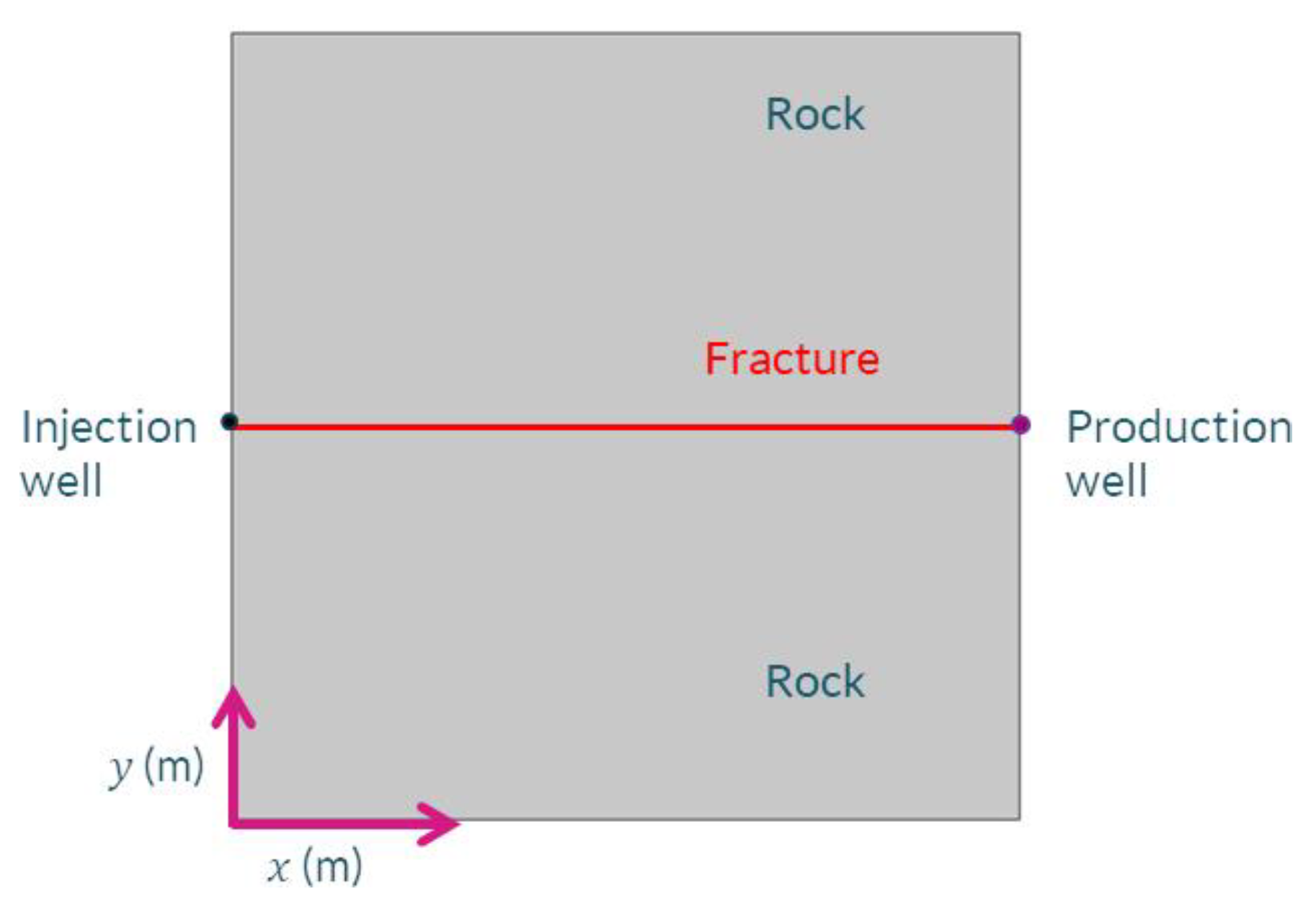
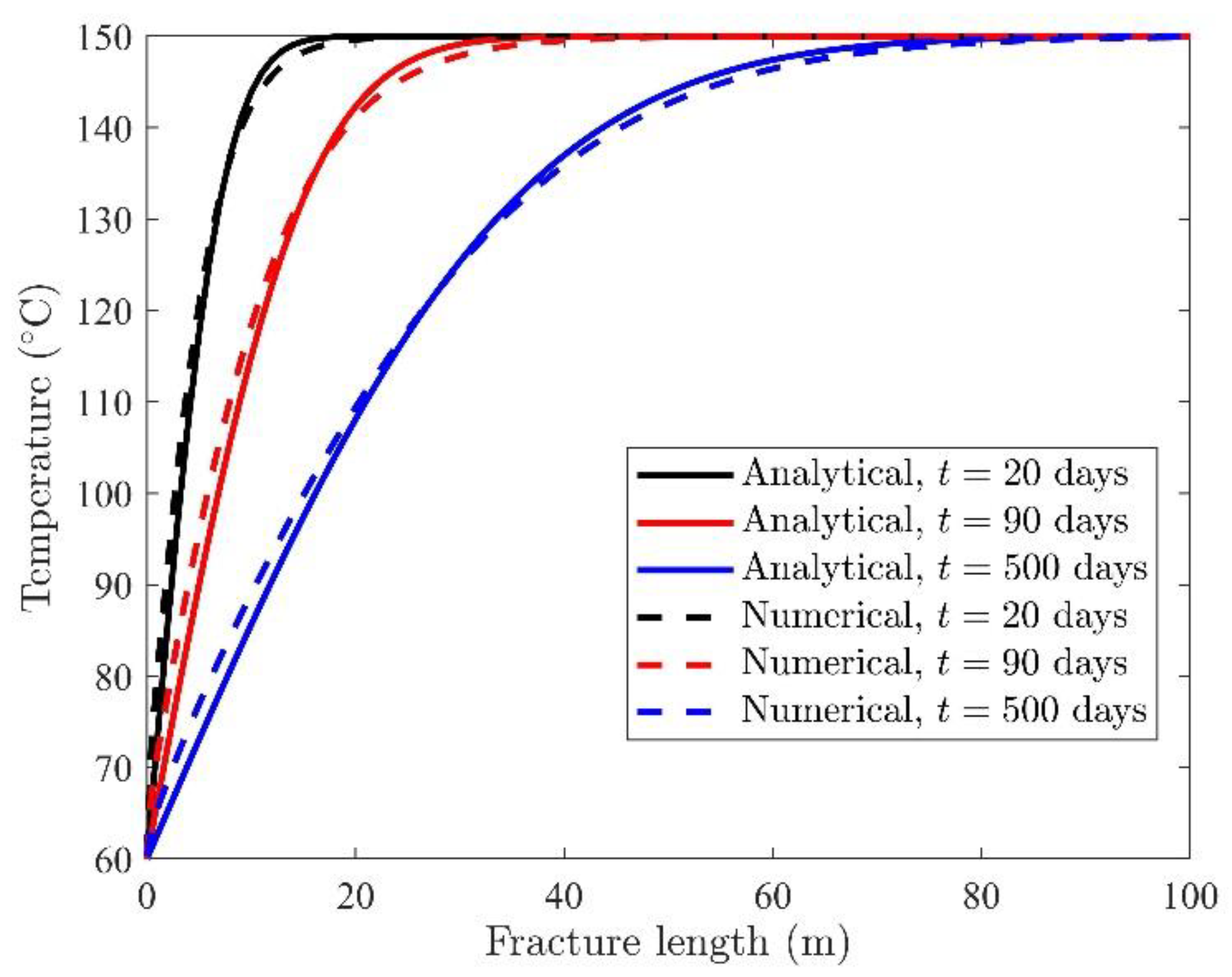
In this section, first we present the benchmark for our numerical model. Then, the hydro-thermal numerical modeling results are compared with the operational data measured at Soultz-sous-Forêts for three years of operation. Furthermore, new injection scenarios are proposed that can be adopted with the existing industrial setup to enhance the energy extraction capability. Finally, we perform sensitivity analysis on ten governing parameters and estimate their impact on the production temperature.

3.1. Benchmarking

For benchmarking the numerical model, we used the approach adopted by Cheng et al. [38] and Bongole et al. [39] by using a simplified 1D heat transfer problem for a single fracture system. This approach is used in the previous studies to benchmark the models. The analytical equation for heat transfer considers that the geometry is infinitely extended in both directions (see Figure 5), there is no flow boundary conditions for heat exchange, steady state fluid flow occurs only through the fracture and the rock permeability is zero, and the thermophysical properties of water are constant throughout the simulation. The temperature distribution for the fluid is identical to that of the rock matrix due to the local thermal equilibrium assumption. The analytical solution for the fluid temperature distribution is [38,39]:

$$T_{fD}\left(x,t\right)=\frac{T_0-T_f\left(x,t\right)}{T_0-T_{in}}=erfc\left[\left(\frac{2{\lambda }_{m}x}{e_h{u}_f\rho C_{p,l}}\right)\sqrt{\frac{u_f{\rho }_m{C}_{p,m}}{4{\lambda }_m\left(u_{f}t-x\right)}}\right]$$

In the above equation, $T_{fD}$ is the nondimensional fracture temperature and $u_f$ is the fluid velocity.

We observe a good agreement between the numerical and analytical solutions, as demonstrated in Figure 6.

The operational data for three years was made available for Soultz-sous-Forêts site by the site operators and is used here to calibrate the coupled unsteady hydro-thermal model. Figure 7 shows the injection and production rates at the wellhead for 1163 days from June 2016 to September 2019. The fluid injection temperature is 70 °C for both the injection wells.

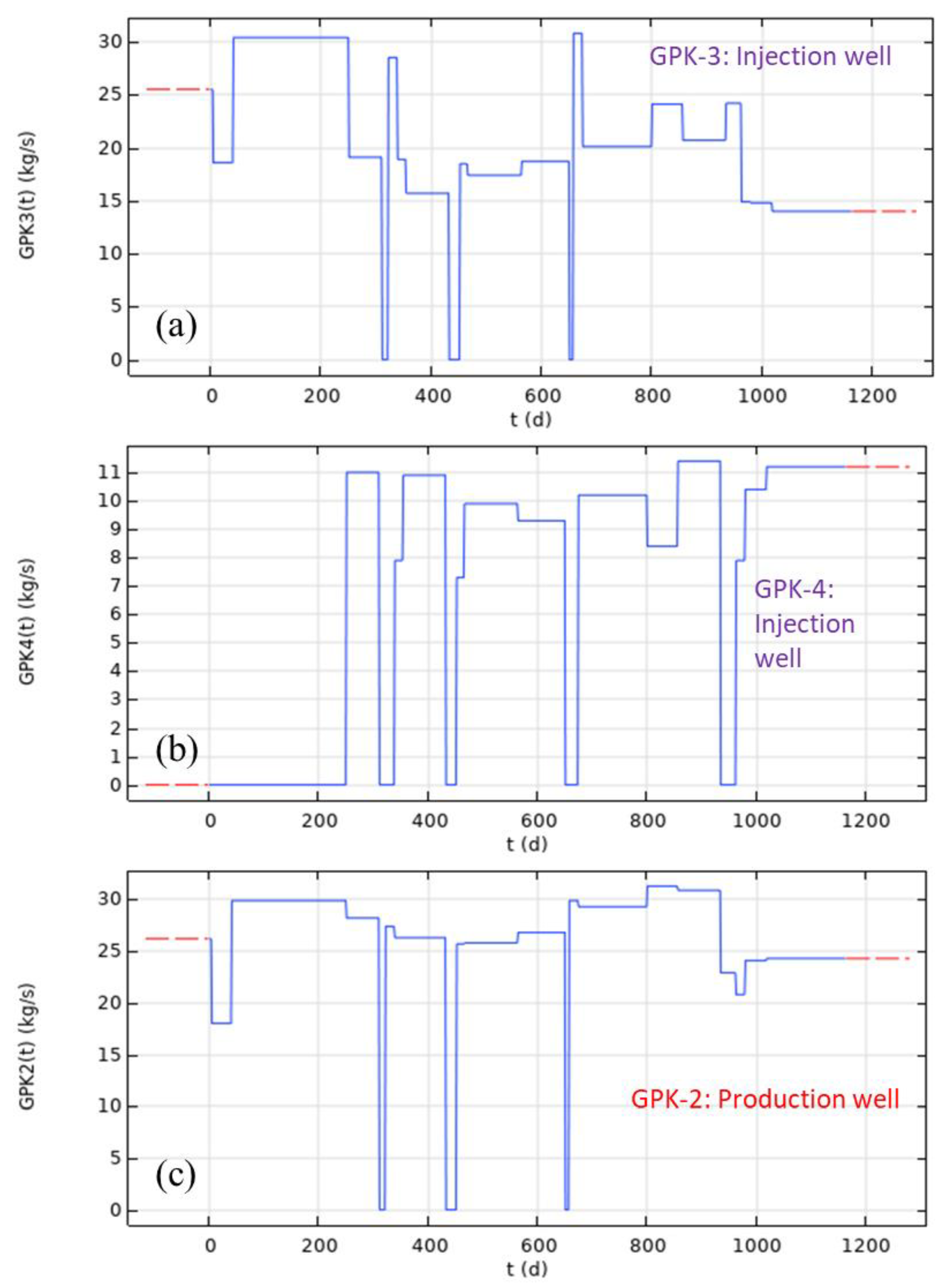
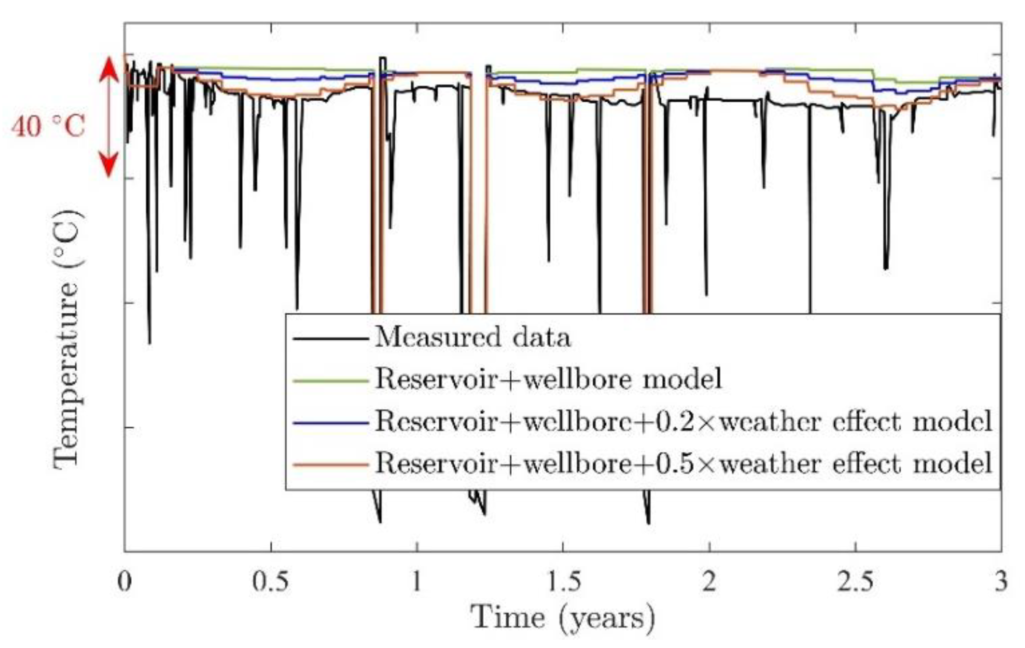
3.2. Validation with Operational Data

In Figure 8, the numerical model data is validated with operational data for the time period as described above. Unfortunately, it is not possible to publish the exact values of operational data due to concerns of our industrial partners and we can only show the amount of change. These are the actual temperature values shown by different colors for operational and simulations (not the differences). The measured temperature data is the operational data for 1163 days at the production wellhead. The temperature at the production well based on the hydro-thermal model is significantly different compared to the operational data. For most of the operational period, the predicted production well temperature is 15 °C higher than the measured temperature. Only operation onset and termination stages display smaller deviation in predicted temperature than observed temperature. Because the wellhead temperature measuring device may be affected by the local ambient temperature and the monthly average temperature near the geothermal site is almost the same for the corresponding months in each operational year, a correction factor to account for the weather impact on the measuring device based on the numerical model is introduced. Two scenarios of seasonal impact on the production fluid temperature are considered: (a) 20% impact of ambient temperature (T_effective=T_simulation + 0.2 × ambient temperature) and (b) 50% impact of ambient temperature (T_effective =T_simulation + 0.5 × ambient temperature).

Figure 8 shows the comparison of the operational data with the coupled reservoir-wellbore model and the weather-influenced production fluid temperature. The integrated wellbore–reservoir model has the highest overestimation of production temperature. However, when daily weather fluctuations in the integrated wellbore–reservoir model are considered, the prediction matches very well for most of the operation, as shown in Figure 8. The temperature differences are more relevant to understand its deviation from the actual value rather than the original temperature. The difference between operational and numerical data while considering 50% of the ambient temperature on the production temperature of the coupled wellbore–reservoir model has the best matching among all models. However, the model deviates by more than 15 °C from the operation data during the periods of 1.8 and 2.4 years. Because no other reasons for these deviations are provided with the operational data set, different measurement procedures or false measurements at the wellhead are assumed as reasons for these deviations.

3.3. Long-Term Operational Behavior

In the next study, the model was extended to a simulation period of 100 years of operation to predict the wellhead temperature development at the production well. In this section, different initial temperatures at the bottom hole section than the operationally measured data were used. The main objective of this study was to estimate the temperature at the production well (GPK-2) for different injection temperatures for long-term operational periods. In both scenarios, the injection rates for the first 1163 days are the same as in the provided operational data set. The recently designed heat exchanger at Soultz-sous-Forêts is capable of cooling the water from 70 to 40 °C using a cooling loop at 15 °C and 40 m³/h [40]. Therefore, two scenarios were considered, A and B, for different injection temperatures. For the remaining operational period, scenario A considers four different fluid injection temperatures at the injection wellhead (70, 60, 50 and 40 °C). The fluid injection rates are 13.3 and 11 L/s for GPK-3 and GPK-4, respectively, and the production fluid rate of GPK-2 is 24.3 L/s for the remaining operational period. In Scenario B, the injection rates after 1163 days are 19.6 and 9.7 L/s for GPK-3 and GPK-4, respectively, and the production rate of GPK-2 is 29.3 L/s; the same four injection wellhead temperatures as for scenario A were considered: 70, 60, 50 and 40 °C. These values of the injection and production rates are the operational requirements requested by our industrial partner.

Figure 9a–d shows the temperature along the wellbore for scenarios A and B, respectively, for both injection wells. The wellbore GPK-3 has an open hole section that causes a linear temperature drop along the wellbore instead of a nonlinear temperature drop, as shown in Figure 9a,b. It is interesting to note that instead of having different injection-production rates in all three wells, the fluid production temperature at the GPK-2 wellhead is almost similar for both of the scenarios A and B, as shown in Figure 9e,f. The small increase in temperature at the production wellhead is due to the sudden drop in the production wellhead pressure. The contribution in the fluid flow is due to the first pressure shock of the injection that comes from the faulted zones which are located at the bottom of the system with a higher temperature. As time proceeds, the contribution from the matrix and the leakage zone increases and reduces the temperature a few days after the beginning of the injection. To calculate the initial temperature at the wellhead, it is assumed that there is a steady state flow from the combination of the matrix and the fault zones. This initial temperature is slightly lower than that of the unsteady condition at the early time period. The fluid with the lower viscosity shows a delay in the development of the pressure shock resulting from the cold fluid injection. Therefore, the contribution from the matrix and the leakage zone for the fluid with the temperature 40 °C happens later and the main fluid flow from the faulted zone in the bottom of the system lasts for a longer time. Moreover, the temperature increase in scenario B is higher compared to that of scenario A due to the fact that scenario B has a higher production rate than scenario A which reduces the time for exchanging heat in the wellbore.

Figure 10 shows the comparison of temperature distribution in the fractures and along the wellbore for scenarios A and B. The higher production rate results in slightly faster thermal drawdown at the production well bottom for scenario B than scenario A. No thermal breakthrough was observed at the production well bottom even after 100 years of operation, as shown in Figure 10e,f.

3.4. Uncertainties

There are several uncertainties in this model. We considered the wellbore as a line source for the heat flow. The faulted zone is formulated using a fracture. Both of these assumptions are reliable because the size of the wellbore and the fault zone is negligible in comparison to the overall size of the reservoir. Data validation for the short operational period for production confirms this behavior. The matrix zone is considered as homogeneous and isotropic. As the permeability of matrix is lower than faulted zone, its contribution to the heat and mass flux is small. Therefore, this assumption holds true. As we do not know the exact point of the leakage zone alongside the casing area, we considered a homogeneous leakage and tried to compensate for the possible errors by performing a trial-and-error method to find an appropriate lumped parameter that defines the wellbore heat exchange effect. Furthermore, due to the unavailability of the geomechanical and geochemical data, we mainly focused on the hydrothermal behavior of the geothermal system. Short-term validation of this TH model gives an insight regarding the accurate system characterization, including the permeability and porosity distribution, fault placement and its contribution to the overall flow, the wellbore effect on the overall heat exchange, and fluid and rock properties. Therefore, it builds a basis for future THM or THMC (thermo-hydro-mechanical-chemical) simulations. Our expectation regarding the THM behavior is that permeability around the injection would increase (resulting from the localized thermoelastic stress reorientation and increased pore pressure). Therefore, the enhanced permeability will be favorable in the energy extraction. Based on this understanding, TH provides a preliminary basis for the thermoelastic and poroelastic stress development in this geothermal site.

3.5. Sensitivity Analysis of Hydrothermal Uncertainties

To examine the effect of the uncertainty of the involved parameters in hydro-thermal simulations for the Soultz-sous-Forêts geothermal reservoir, a detailed sensitivity analysis was performed, and its results are shown in Figure 11. The base case was selected as scenario A with an injection temperature of 40 °C. The range of parameters are mentioned in

Table 3. Range of parameters for sensitivity analysis.

Parameter	Base Case Value	1st Assumed Value	2nd Assumed Value
Matrix hydraulic conductivity	$9\times {10}^{-9}$ m/s	$0.5\times 9\times {10}^{-9}$ m/s	$2\times 9\times {10}^{-9}$ m/s
Heat flux from the bottom boundary	0.07 W/m2	0.1 W/m2	0.15 W/m2
Matrix specific heat capacity	1115 J/kg/K	1090 J/kg/K	1140 J/kg/K
Hydraulic conductivity of fault zone (see Table 2)	$K_{f,0}$ m/s	$0.5K_{f,0}$ m/s	$2K_{f,0}$ m/s
Porosity of the fault zone	0.1	0.05	0.2
Wellbore leakage fraction	65%	60%	70%
Matrix porosity	0.03	0.01	0.05
Thermal conductivity of the matrix	2.5 W/m/K	2 W/m/K	3 W/m/K
Fault thickness (see Table 2)	$F_0$ m	$0.5F_0$ m	$2F_0$ m
Thermal conductivity of the fault zone	2.5 W/m/K	2 W/m/K	3 W/m/K

. Results show that the hydraulic conductivity of the matrix and fault zone and the wellbore leakage have a considerable effect on the production temperature. This finding is well aligned with the sensitivity analysis of the THM process in the fracture reservoir system [41,42]. However, these values are one order of magnitude lower than the wellbore heat exchange effect, as shown in Figure 9e. The other three parameters—fault thickness, matrix thermal conductivity and the matrix specific heat capacity—have approximately 1 °C variation over 100 years of operation. The porosity of the matrix and the fault zone, in addition to the fault zone thermal conductivity, have no impact on the temperature variation. Interestingly, heat flux has no effect on the production temperature at the surface due to the conductive heat flow in the reservoir and because the fault zones are farther away from the bottom boundary considered for the simulation. Important parameters in this sensitivity analysis show a monotonic effect on the production temperature behavior and they cannot explain the sinusoidal temperature fluctuation of more than 10 °C in each year. To check our assumption regarding the weather fluctuation impact on the production temperature, we tried to estimate the wellbore heat exchange effect. We found that the wellbore heat exchange is mainly flow-rate dependent parameter and the flow rates for the production data are constant from 41 to 250 days, whereas we can see a fluctuation in the recorded temperature. This indicates that the cyclic variability in the production temperature cannot be supported by the wellbore heat exchange argument. Therefore, the most suitable reason of the periodic production temperature variability is weather fluctuation on the measuring device.

4. Conclusions

As part of the MEET project, a coupled reservoir and wellbore model for hydraulic and thermal processes involved during the geothermal energy extraction operation at Soultz Sous Forêts was developed. Operational data from a period of 1163 days of operation was used to validate the numerical model. The validated hydro-thermal numerical model precisely simulates the geothermal energy extraction operation for 3 years. Furthermore, two operational scenarios for 100 years with four different injection wellhead temperatures—70, 60, 50 and 40 °C—were analyzed. It can be observed that even after 100 years of operation, the thermal breakthrough at the production well is only in the range of 10 to 20 °C. After 100 years of cold fluid injection and hot fluid production, the observed temperature drop at the production wellhead is less than 20 °C. Therefore, our numerical model predicts that 100 years of geothermal energy extraction operation at Soultz-sous-Forêts is feasible and will have a sufficiently high production temperature throughout the operation duration.

References

1. COP-21. Paris Agreement, United Nations Framework Convention on Climate Change, Conference of the Parties 21. Available online: https://unfccc.int/process-and-meetings/the-paris-agreement/the-paris-agreement (accessed on 15 June 2021).
2. Mahmoodpour, S.; Amooie, M.A.; Rostami, B.; Bahrami, F. Effect of gas impurity on the convective dissolution of CO2 in porous media. Energy 2020, 199, 117397. [Google Scholar] [CrossRef]
3. Mahmoodpour, S.; Rostami, B.; Soltanian, M.R.; Amooie, A. Convective dissolution of carbon dioxide in deep saline aquifers: Insights from engineering a high-pressure porous cell. Phys. Rev. Appl. 2019, 12, 034016. [Google Scholar] [CrossRef] [Green Version]
4. Singh, M.; Chaudhuri, A.; Stauffer, P.H.; Pawar, R.J. Simulation of gravitational instability and thermo-solutal convection during the dissolution of CO2 in deep storage reservoirs. Wat. Resour. Resear. 2020, 56, e2019WR026126. [Google Scholar]
5. Singh, M.; Tangirala, S.K.; Chaudhuri, A. Potential of CO2 based geothermal energy extraction from hot sedimentary and dry rock reservoirs, and enabling carbon geo-sequestration. Géoméch. Geophys. Geo. Energy Geo. Resour. 2020, 6, 16. [Google Scholar] [CrossRef]
6. Singh, M.; Chaudhuri, A.; Soltanian, M.R.; Stauffer, P.H. Coupled multiphase flow and transport simulation to model CO2 dissolution and local capillary trapping in permeability and capillary heterogeneous reservoir. Int. J. Greenh. Gas Control. 2021, 108, 103329. [Google Scholar] [CrossRef]
7. EGEC Geothermal. The Geothermal Energy Market Grows Exponentially, but Needs the Right Market Conditions to Thrive. Available online: https://www.egec.org/the-geothermal-energy-market-grows-exponentially-but-needs-the-right-market-conditions-to-thrive/ (accessed on 15 June 2021).
8. Longa, F.D.; Nogueira, L.P.; Limberger, J.; van Wees, J.-D.; van der Zwaan, B. Scenarios for geothermal energy deployment in Europe. Energy 2020, 206, 118060. [Google Scholar] [CrossRef]
9. MEET. (N.D.). Multidisciplinary and Multi-Context Demonstration of Enhanced Geothermal Systems Exploration and Exploitation Techniques and Potentials, European Union’s Horizon 2020 Research and Innovation Program under Grant Agreement No. 792037. Available online: https://www.meet-h2020.com/ (accessed on 15 October 2021).
10. Duringer, P.; Aichholzer, C.; Orciani, S.; Genter, A. The complete lithostratigraphic section of the geothermal wells in Rittershoffen (Upper Rhine Graben, eastern France): A key for future geothermal wells. BSGF Earth Sci. Bull. 2019, 190, 13. [Google Scholar] [CrossRef] [Green Version]
11. Cocherie, A.; Guerrot, C.; Fanning, C.M.; Genter, A. Datation U–Pb Des Deux Faciès Du Granite de Soultz (Fossé Rhénan, France). Comptes Rendus Geosci. 2004, 336, 775–787. [Google Scholar] [CrossRef]
12. Schill, E.; Genter, A.; Cuenot, N.; Kohl, T. Hydraulic performance history at the Sultz EGS reservoirs from stimulation and long term circulation tests. Geothermics 2017, 70, 110–124. [Google Scholar] [CrossRef]
13. Rolin, P.; Hehn, R.; Dalmais, E.; Genter, A. D3.3 Hydrothermal Model Matching Colder Reinjection Design, WP3: Upscaling of Thermal Power Production and Optimized Operation of EGS Plants. 2018, H2020 Grant Agreement No-792037, Report. Available online: https://cordis.europa.eu/project/id/792037/reporting (accessed on 10 April 2021).
14. Vallier, B.; Magnenet, V.; Schmittbuhl, J.; Fond, C. THM modeling of gravity anamolies related to deep hydrothermal circulation at Soultz-sous-Forêts (France). Geotherm. Energy 2020, 8, 13. [Google Scholar] [CrossRef]
15. Genter, A.; Guillou-Frottier, L.; Feybesse, J.-L.; Nicol, N.; Dezayes, C.; Schwartz, S. Typology of potential Hot Fractured Rock resources in Europe. Geothermics 2003, 32, 701–710. [Google Scholar] [CrossRef]
16. Bächler, D.; Kohl, T.; Rybach, L. Impact of graben-parallel faults on hydrothermal convection––Rhine Graben case study. Phys. Chem. Earth Parts A B C 2003, 28, 431–441. [Google Scholar] [CrossRef]
17. Kohl, T.; Bächler, D.; Rybach, L. Steps towards a comprehensive thermo-hydraulic analysis of the HDR test site Soultz-sous-Forêts. In Proceedings of the World Geothermal Congress, Beppu/Morioka, Japan, 28 May–10 June 2000; pp. 2671–2676. [Google Scholar]
18. Pribnow, D.; Schellschmidt, R. Thermal tracking of upper crustal fluid flow in the Rhine graben. Geophys. Res. Lett. 2000, 27, 1957–1960. [Google Scholar] [CrossRef]
19. Baillieux, O.; Schill, E.; Edel, J.-B.; Mauri, G. Localization of temperature anomalies in the Upper Rhine Graben: Insights from geophysics and neotectonics activity. Int. Geol. Rev. 2013, 55, 1744–1762. [Google Scholar] [CrossRef]
20. GeORG. Potentiel Géologique Profond du Fossé Rhénan Supérieur. Parties 1 à 4. 2013. Available online: http://www.geopotenziale.eu (accessed on 10 April 2021).
21. Surma, F.; Geraud, Y. Porosity and Thermal Conductivity of the Soultz-sous-Forêts Granite. Pure Appl. Geophys. 2003, 160, 1125–1136. [Google Scholar] [CrossRef]
22. Vallier, B.; Magnenet, V.; Schmittbuhl, J.; Fond, C. Large scale hydro-thermal circulation in the deep geothermal reservoir of Soultz-sous-Forêts (France). Geothermics 2019, 78, 154–169. [Google Scholar] [CrossRef]
23. Sausse, J.; Dezayes, C.; Dorbath, L.; Genter, A.; Place, J. 3D model of fracture zones at Soultz-sous-Forêts based on geological data, image logs, induced microseismicity and vertical seismic profiles. Comptes Rendus Geosci. 2010, 342, 531–545. [Google Scholar] [CrossRef]
24. Dezayes, C.; Genter, A.; Valley, B. Structure of the low permeable naturally fractured geothermal reservoir at Soultz. Comptes Rendus Geosci. 2010, 342, 517–530. [Google Scholar] [CrossRef] [Green Version]
25. Guillou-Frottier, L.; Carrė, C.; Bourgine, B.; Bouchot, V.; Genter, A. Structure of hydrothermal convection in the Upper Rhine Graben as inferred from corrected temperature data and basin-scale numerical models. J. Volcanol. Geotherm. Res. 2013, 256, 29–49. [Google Scholar] [CrossRef] [Green Version]
26. Gérard, A.; Genter, A.; Kohl, T.; Lutz, P.; Rose, P.; Rummel, F. The deep EGS (enhanced geothermal system) project at soultz-sous-Forêts (Alsace, France). Geothermics 2006, 35, 473–483. [Google Scholar] [CrossRef]
27. Sanjuan, B.; Pinault, J.L.; Rose, P.; Gerard, A.; Brach, M.; Braibant, G.; Crouzet, C.; Foucher, J.C.; Gautier, A. Geochemical fluid characteristics and main achievements about traces tests at Soultz-sous-Forêts (France). In Proceedings of the EHDRA Scientific Conference 2006, Soultz-sous-Forêts, France, 15–16 June 2006. [Google Scholar]
28. Blumenthal, M.; Kuhn, M.; Pape, H.; Rath, V.; Clauser, C. Hydraulic model of the deep reservoir quantifying the multi-well tracer test. In Proceedings of the EHDRA Scientific Conference, Soultz-sous-Forêts, France, 28–29 June 2007. [Google Scholar]
29. Gessner, K.; Kühn, M.; Rath, V.; Kosack, C.; Blumenthal, M.; Clauser, C. Coupled Process Models as a Tool for Analysing Hydrothermal Systems. Surv. Geophys. 2009, 30, 133–162. [Google Scholar] [CrossRef]
30. Egert, R.; Maziar, G.K.; Held, S.; Kohl, T. Implications on large-scale flow of the fractured EGS reservoir Soultz inferred from hydraulic data and tracer experiments. Geothermics 2020, 84, 101749. [Google Scholar] [CrossRef]
31. Gentier, S.; Rachez, X.; Ngoc, T.D.T.; Peter-Borie, M.; Souque, C. 3D flow modelling of the medium-term circulation test performed in the deep geothermal site of Soultz-sous-Forêts (France). In Proceedings of the World Geothermal Congress, Bali, Indonesia, 25–30 April 2010; p. 13. [Google Scholar]
32. Magnenet, V.; Fond, C.; Genter, A.; Schmittbuhl, J. Two-dimensional THM modelling of the large scale natural hydrothermal circulation at Soultz-sous-Forêts. Geotherm. Energy 2014, 2, 533. [Google Scholar] [CrossRef] [Green Version]
33. Aliyu, M.D.; Chen, H. Numerical modelling of coupled hydro-thermal processes of the Soultz heterogeneous geothermal system. In Proceedings of the Seventh European Congress on Computational Methods in Applied Sciences and Engineering ECCOMAS Congress Stanford University, Crete Island, Greece, 5–10 June 2016. [Google Scholar]
34. COMSOL Multiphysics® v. 5.6. COMSOL AB: Stockholm, Sweden. Available online: www.comsol.com (accessed on 11 November 2020).
35. Alves, I.; Alhanati, F.; Shoham, O. A Unified Model for Predicting Flowing Temperature Distribution in Wellbores and Pipelines. SPE Prod. Eng. 1992, 7, 363–367. [Google Scholar] [CrossRef]
36. Hasan, A.R.; Kabir, C.S.; Wang, X. A Robust Steady-State Model for Flowing-Fluid Temperature in Complex Wells. SPE Prod. Oper. 2009, 24, 269–276. [Google Scholar] [CrossRef]
37. Moradi, B.; Ayoub, M.; Bataee, M.; Mohammadian, E. Calculation of temperature profile in injection wells. J. Pet. Explor. Prod. Technol. 2020, 10, 687–697. [Google Scholar] [CrossRef] [Green Version]
38. Bongole, K.; Sun, Z.; Yao, J.; Mehmood, A.; Yueying, W.; Mboje, J.; Xin, Y. Multifracture response to supercritical CO2-EGS and water-EGS based on thermo-hydro-mechanical coupling method. Int. J. Energy Res. 2019, 43, 7173–7196. [Google Scholar]
39. Cheng, A.H.-D.; Ghassemi, A.; Detournay, E. Integral equation solution of heat extraction from a fracture in hot dry rock. Int. J. Numer. Anal. Methods Géoméch. 2001, 25, 1327–1338. [Google Scholar] [CrossRef]
40. Ravier, G. Deliverable, D.3.1, Design of a Heat Exchanger for Cold Injection, WP3: Upscaling of Thermal Power Production and Optimized Operation of EGS Plants, Report Submitted to European Union. 2019. Available online: https://www.meet-h2020.com/project-results/deliverables/ (accessed on 11 November 2020).
41. Mahmoodpour, S.; Singh, M.; Turan, A.; Bär, K.; Sass, I. Key parameters affecting the performance of fractured geothermal reservoirs: A sensitivity analysis by thermo-hydraulic-mechanical simulation. arXiv 2021, arXiv:2107.02277. [Google Scholar]
42. Mahmoodpour, S.; Singh, M.; Bär, K.; Sass, I. Thermo-hydro-mechanical modeling of an enhanced geothermal system in a fractured reservoir using CO2 as heat transmission fluid—A sensitivity investigation. arXiv 2021, arXiv:2108.05243. [Google Scholar]
Figure 1. Temperature distribution at 2 km depth TVD in the Upper Rhine Graben [19].
Geosciences 11 00464 g001
Figure 2. Geothermal gradient at the Soultz-sous-Forêts site. Here, an anomaly in temperature is observable in the top 3 km section or in the sedimentary layer. We assumed 10 °C temperature at the surface to calculate this geothermal gradient. The initial data up to the depth of 5.1 km is measured alongside GPK-2 by Pribnow and Schellschmidt [25] and further modified by Rolin et al. [13].
Geosciences 11 00464 g002
Figure 3. Geometry for numerical modeling of Soultz-sous-Forêts geothermal site. Elliptic geometries are faults listed in Table 1 (blue color). Open hole sections of the injection wells are denoted by green colors (GPK-3 and GPK-4) whereas open hole section of the production well is denoted by the dark red color (GPK-2). The leakage zone of the production well is denoted by light red whereas the leakage zone of the GPK-3 is shown by the yellow color.
Geosciences 11 00464 g003
Figure 4. Wellbore heat loss modeling schematic.
Geosciences 11 00464 g004
Figure 5. Geometry for the benchmarking problem.
Geosciences 11 00464 g005
Figure 6. Comparison of the numerical solution with the analytical temperature distribution along the fracture length.
Geosciences 11 00464 g006
Figure 7. Injection schedule at (a) GPK-3 and (b) GPK-4 and (c) production schedule at production well GPK-2 for 1163 days of operation from June 2016 to September 2019. Here, the blue lines are the actual injection and production rates. The red dash lines indicate no operation period.
Geosciences 11 00464 g007
Figure 8. Difference between operational data from June 2016 to September 2019 and the data obtained from the numerical model.
Geosciences 11 00464 g008
Figure 9. Comparison between scenarios A and B for (a,b) temperature along the injection well GPK-3, (c,d) temperature along the injection well GPK-4, and (e,f) wellhead temperature at the production well GPK-2.
Geosciences 11 00464 g009
Figure 10. Comparison of temperature distribution (in SI units) in the fractures for scenarios A and B at time (a,b) 0 year, (c,d) 50 years and (e,f) 100 years. Here, Δ T is the temperature drop in the reservoir from the initial state.
Geosciences 11 00464 g010
Figure 11. Sensitivity analysis for 10 parameters affecting the hydro-thermal processes at Soultz-sous-Forêts for (a) matrix hydraulic conductivity, (b) heat flux from the bottom boundary, (c) matrix specific heat capacity, (d) hydraulic conductivity of faults (here K f , 0 is the fault zone hydraulic conductivity as given in Table 2), (e) porosity of fault zone, (f) leakage contribution to the total fluid flow, (g) matrix porosity, (h) matrix thermal conductivity, (i) fault thickness (here F 0 is the fault thickness as given in Table 2), and (j) thermal conductivity of the fault zone.
Geosciences 11 00464 g011