Abstract
The purpose of the work presented in this paper is to study the reflection and transmission coefficients resulting from the interactions of regular waves with a rectangular breakwater sited at the bottom of a tank. The present investigation is devoted to the analysis of the reflection and transmission coefficients within the framework of linearized potential flow theory using two methods, a numerical method based on the improved version of the meshless singular boundary method, and the analytical approach within the plane wave model. The numerical method is first validated by studying the accuracy of the numerical computations with respect to the number of boundary nodes and the location of the vertical boundaries of the computational domain, for different immersion ratios (h/d) and different relative lengths (w/d) of the obstacle. To assess the limitations of the analytical approach, a comparison analysis is carried out between the analytical and numerical results. To improve the calculations and the effectiveness of the analytical model, slight adjustments are made to the analytical procedure, which is termed here the corrected analytical plane wave model. Finally, the effects of the immersion ratio (h/d) and the relative length (w/d) of the obstacle on the reflection and transmission coefficients are computed using the three methods, and discussed for several wave and structural conditions.
1. Introduction
The coast is a site where several phenomena can appear and affect coastal structures, such as sea-level rise caused by climate change, erosion due to wave actions, and the decrease of fluvial sediment supply caused by the construction of dams, etc. Consequently, researchers, engineers, and scientists have shown that the reflection of swell is one of the convincing and relevant solutions to overcome problems of erosion, surges, marine submersions, and all phenomena to which these structures can be exposed. Therefore, the maximization of wave reflection has become extremely important in coastal engineering, and arouses the interest of many researchers in the literature to investigate the numerical, experimental, and theoretical methods that can study the reflection of wave–structure interactions.
Considerable research has been carried out in the past on different types of breakwaters. Nevertheless, the operating conditions of breakwaters are very challenging and, hence, there is still a need for additional research to fill in the gaps. A short account of what has been delivered up till now is given here. Dean [1] studied the effect of the wave amplitudes on the reflection of surface waves by a submerged plane barrier. Takano [2] evaluated the passage effect of waves propagating under a rectangular breakwater. Patarapanich [3] studied the wave reflection and transmission by a submerged thin horizontal plate using the finite element method (FEM). Using the matched asymptotic method, Liu and Jiankng [4] investigated the transmitted wave intensity through a submerged slit on a vertical barrier. On the other hand, using a parametric experimental design, Stamos et al. [5] compared the reflection and transmission coefficients resulting from the interaction of waves with a variety of submerged water-filled breakwater models of hemi-cylindrical and rectangular shapes. Molin et al. [6] carried out laboratory experiments to investigate the interaction of waves with a rigid vertical plate. Shortly afterwards, Lui et al. [7] examined the Bragg reflections of water waves by multiple submerged semi-circular breakwaters.
Further, the submerged rectangular step is a structure mostly used as a breakwater to protect shorelines by diminishing the destructive effects of the wave actions, reducing the erosion of coasts, and protecting coastal structures from damage [8]. Recently, the rectangular submerged breakwater has started to receive more attention compared to the traditional emerged structures, due to its attractive aesthetics and ability to allow water circulation as well as the passage of fish. Several experimental, analytical, and numerical studies have been devoted to studying the reflection and transmission of swells by this type of structure. Mei and Black [9] studied the problem of scattering properties for bottom and surface obstacles using the variational method. Massel [10] investigated the interaction of waves with an infinite- and finite-length rectangular submerged breakwater. Andrew et al. [11] presented an experimental and numerical study based on the boundary element method (BEM) to investigate the propagation of waves over a submerged impermeable obstacle of a rectangular cross section. Recently, Szmidt [12] studied numerically using the finite difference method (FDM), the interaction of waves with a rectangular breakwater fixed at the bottom of numerical wave tank (NWT), and estimated the efficiency of the breakwater in protecting sea shelf zones from open sea waves.
We propose to investigate, in this paper, the capabilities of the improved version of the meshless singular boundary method (ISBM) [13,14,15] to analyze the reflection and transmission coefficients resulting from the interactions of regular waves with a rectangular breakwater sited at the bottom of a tank. The method is validated by studying the accuracy of the numerical results with respect to the number of boundary nodes and the location of the vertical boundaries of the computational domain for different immersion ratios (h/d) and different relative lengths (w/d) of the obstacle. Further, the analytical reflection and transmission coefficients within the plane wave model (see Appendix A) are compared with the results of the numerical model and discussed for several wave and structural conditions. To improve the shortfalls of the analytical model, slight modifications are introduced to the analytical procedure, which is termed here the corrected analytical plane wave model. Finally, a general discussion is made to highlight the strengths and limitations of the corrected plane wave model.
This paper is divided into five main sections. After presenting the introduction of the work and stating the objective of this research in Section 1, the formulation of the problem and the numerical method used in this work are presented in Section 2 and Section 3. In Section 4, the error sensitivity indicator, and comparisons of the numerical and analytical results and analysis, are presented to study the interactions of regular waves with a rectangular breakwater sited at the bottom of a tank. Finally, some conclusions and perspectives are illustrated in Section 5.
2. Formulation of the Problem
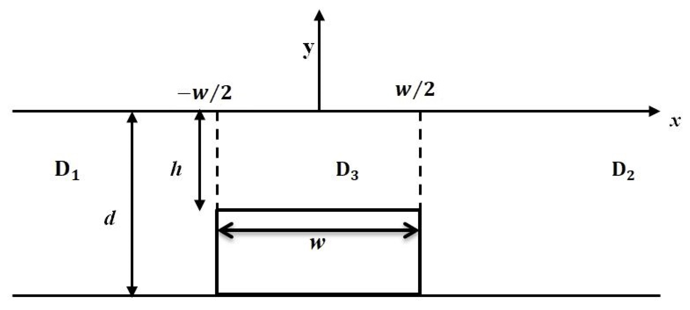
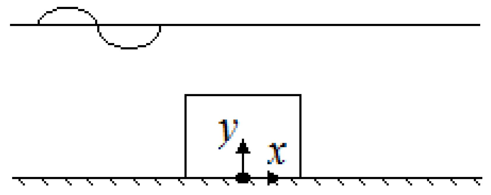
We consider, in this study, a submerged single impermeable rectangular step (breakwater) which is placed at the bottom, as shown in Figure 1.
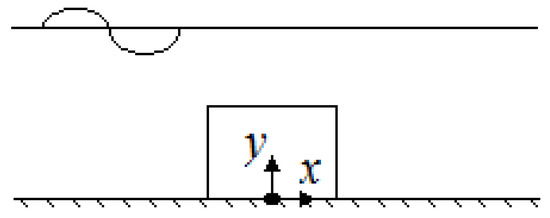
Figure 1.
Breakwater system of this study.
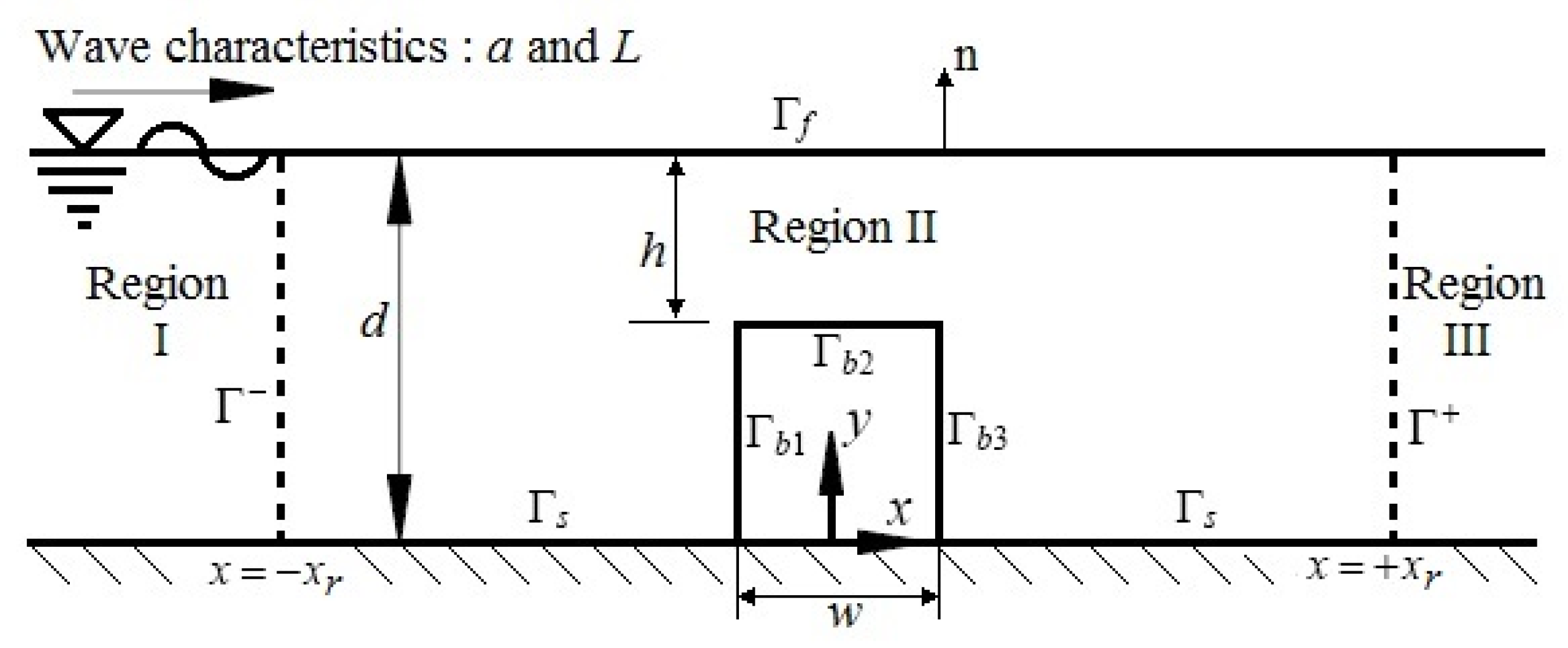
The idealized geometry of the two-dimensional (2D) problem in a Cartesian system (x-y) is shown in Figure 2. Regular waves of small amplitude a, period T, and wavelength L impinge from the left in water of depth d. Assuming an irrotational flow and incompressible fluid motion, the problem is formulated using a velocity potential where Re denotes the real part, is the time independent spatial velocity potential, is the wave angular frequency, and t is the time. The wave number is the solution of the dispersion relation , where g is the gravitational acceleration. The wave field is totally specified if the two-dimensional velocity potential is known.
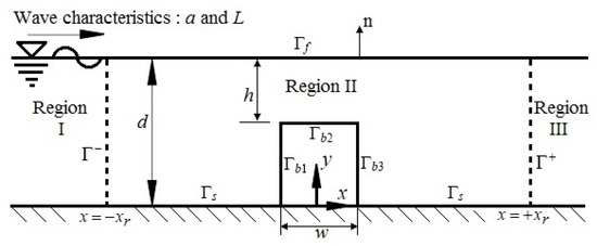
Figure 2.
Problem definitions for the breakwater system.
The breakwater is described by the immersion ratio h/d and relative length (w/d), where d is the water depth in the absence of the obstacle, h is the water depth above the obstacle, and w is the length of the obstacle.
The total fluid domain is divided into three regions as shown in Figure 2. Region I at (−∞) is the region where the waves are incoming (inflow), and region III at (+∞) is where the waves are transmitted (outflow). Region II is between regions I and III, and is delimited by the rigid (impermeable) walls of the breakwater (, , and ), the free surface boundary , the seabed boundary , and the radiation boundaries and , respectively, of the inflow and outflow regions. The spatial velocity potential satisfies the following conditions:
where n is the normal to the boundary pointing out of the flow region, and denotes the total rigid (impermeable) boundary of the breakwater.
The radiation conditions at the inflow and outflow regions are expressed as
where is the incident velocity potential.
The radiation conditions in the infinite strip problem are treated by transferring the far field potentials at two fictitious vertical boundaries at finite distances and , representing, respectively, the left boundary and the right boundary of the fluid domain. The analytical series at these boundaries are given by:
where and are unknown complex coefficients to be determined. The disturbances are guaranteed to be out-going waves only (see for example [16,17]). The incident velocity potential is defined as:
The special matching conditions at the interfaces and of the flow regions ensure a smooth transfer of the mass flow from one region to the next. Once the potentials and are calculated by satisfying the radiation boundary conditions of Equations (5) and (6), they are matched to those of Equations (7) and (8), then the unknown coefficients and are evaluated following the method of Yueh and Chuang [18]:
where .
The reflection and transmission coefficients (R and ) are determined from the following expressions (see [16,17] and further details in Appendix B):
3. Numerical Solution by the ISBM
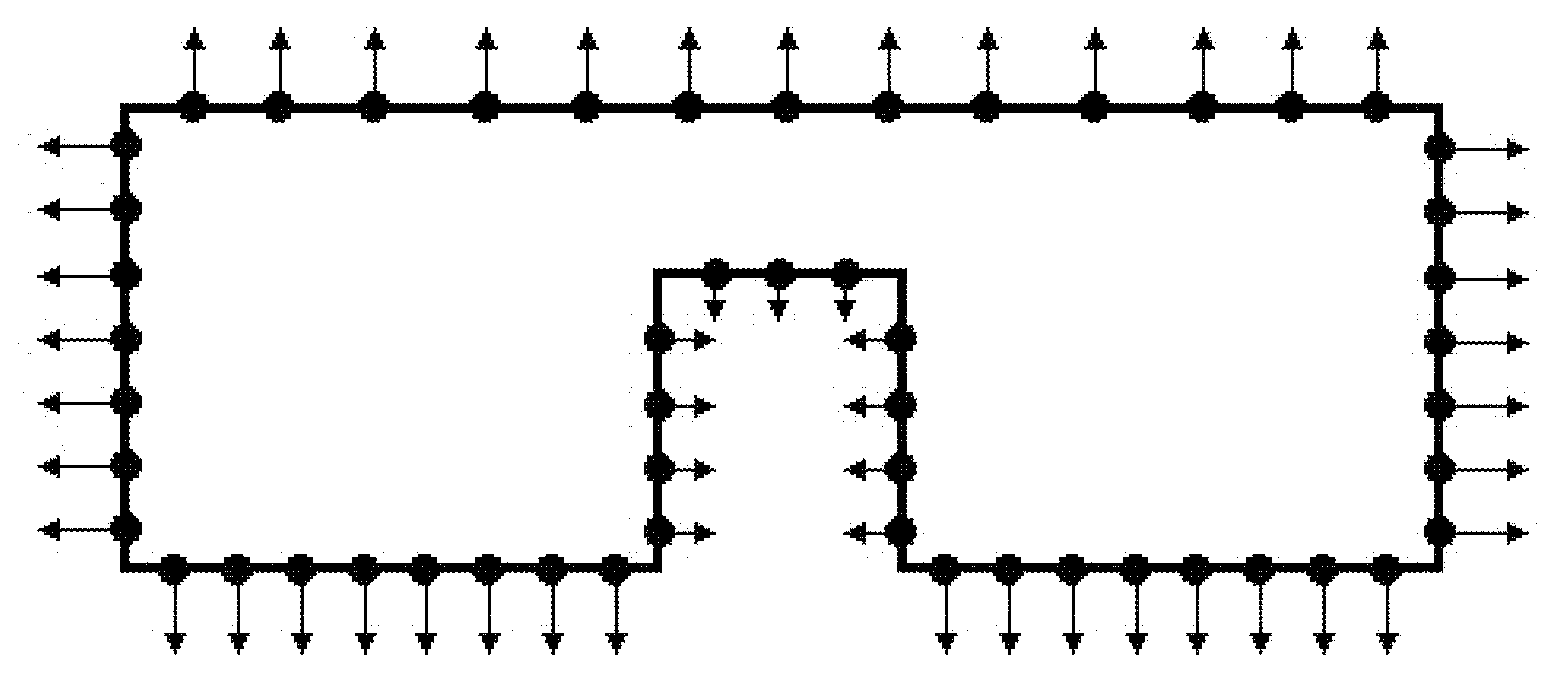
For the numerical solution the total boundary of the whole computational domain is discretized as shown in Figure 3 for the single breakwater.
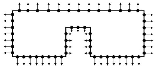
Figure 3.
Domain discretization.
In the ISBM, the nodal values of the potentials and their fluxes are expressed as linear combinations of fundamental solutions and their derivatives [13,14,15],
where are unknown coefficients to be determined, and are, respectively, the collocation points and the source points , and N is the total number of points. and are the Dirichlet and Neumann values, and is the normal at the collocation point . The coefficients and are source intensity factors corresponding, respectively, to the fundamental solution and its derivative. is the fundamental solution of the 2D Laplace equation. It depends only on the Euclidean distance between the collocation points and the source points , i.e., , and is given together with its normal derivative as:
and are the component of the normal at the collocation point .
The coefficients and are the diagonal elements of the ISBM interpolation matrices. They arise when the collocation points and the source points coincide (). Direct evaluation of these coefficients is unfeasible because of the singularities inherent in the fundamental solution and its derivative. In this study, the coefficients are evaluated simply by the integration of the fundamental solution on line segments leading to a simple analytical expression as [19,20]:
For the coefficient , a simple expression is derived by Gu [14], using a regularization process of subtracting and adding-back to remove singularities:
where and are the half distances, respectively, between the collocations points and , and the source points and . is the normal at the source point .
The boundary conditions given by Equations (2)–(6) are satisfied by a linear combination of Equations (13) and (14). The discretization process leads to:
For nodes (free surface boundary):
For nodes (the radiation boundary at ):
For nodes (the radiation boundary at ):
For nodes and (seabed and breakwater boundaries):
The resulting discretized Equations (19)–(22) are written in a more compact matrix form as:
where N is the total number of nodes on the whole domain boundaries, e.g., , where , , , , and are the number of nodes respectively on the boundaries , , , , and . The algebraic system of equations expressed by Equation (23) is solved numerically using a Gaussian elimination algorithm to yield the vector of unknowns . The potential and its derivative at the nodes are then computed using Equations (13) and (14).
4. Results and Discussion
The results of the present investigation are divided into two separate sections. The first section is dedicated to studying the sensitivity of the numerical results of the ISBM to ensure the validity of the proposed numerical wave model. In the Section 2, comparison is made between the results of the ISBM, the analytical approach within the plane wave model (see Appendix A), and the corrected plane wave model.
4.1. Error Indicators Analysis
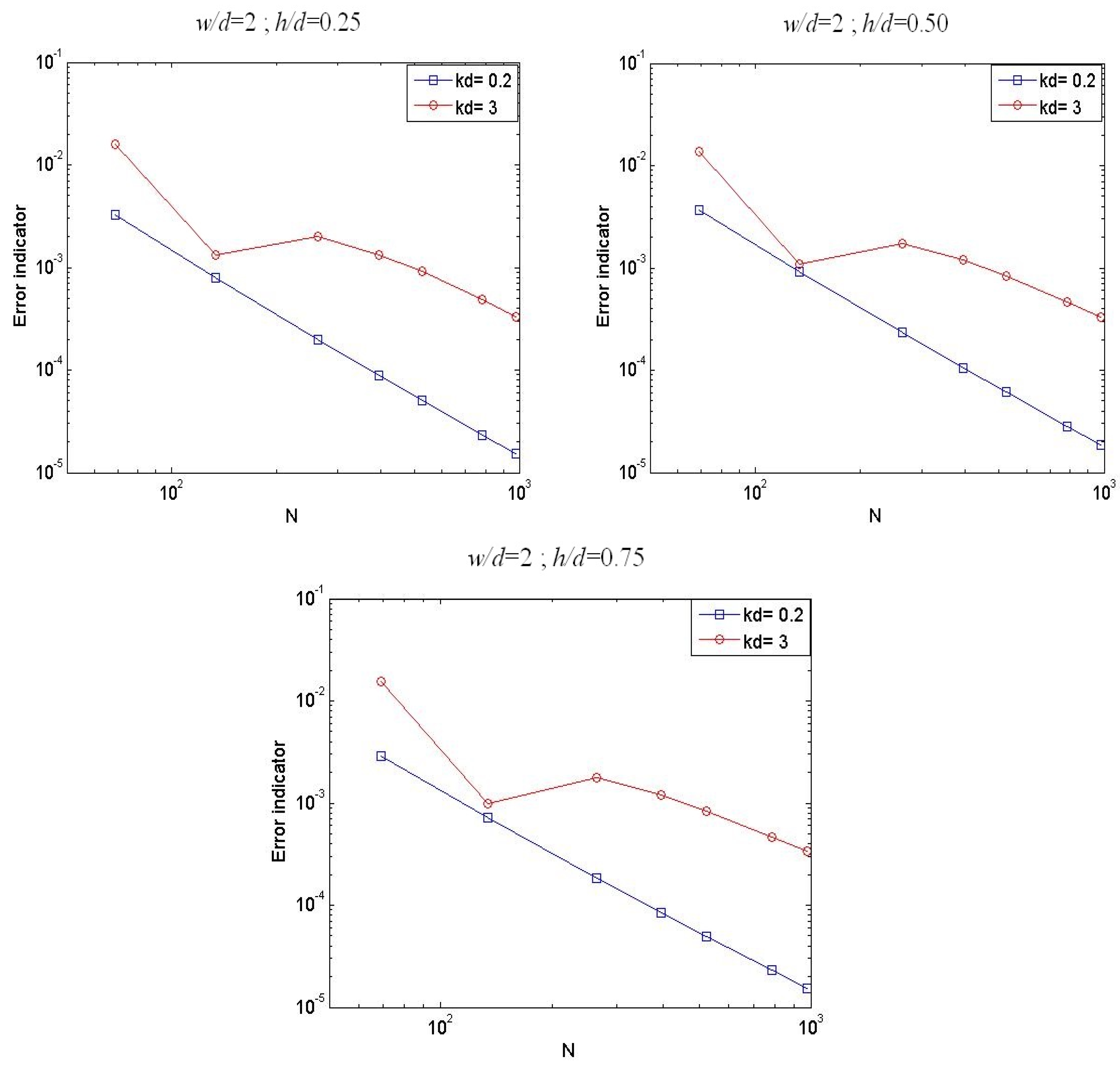
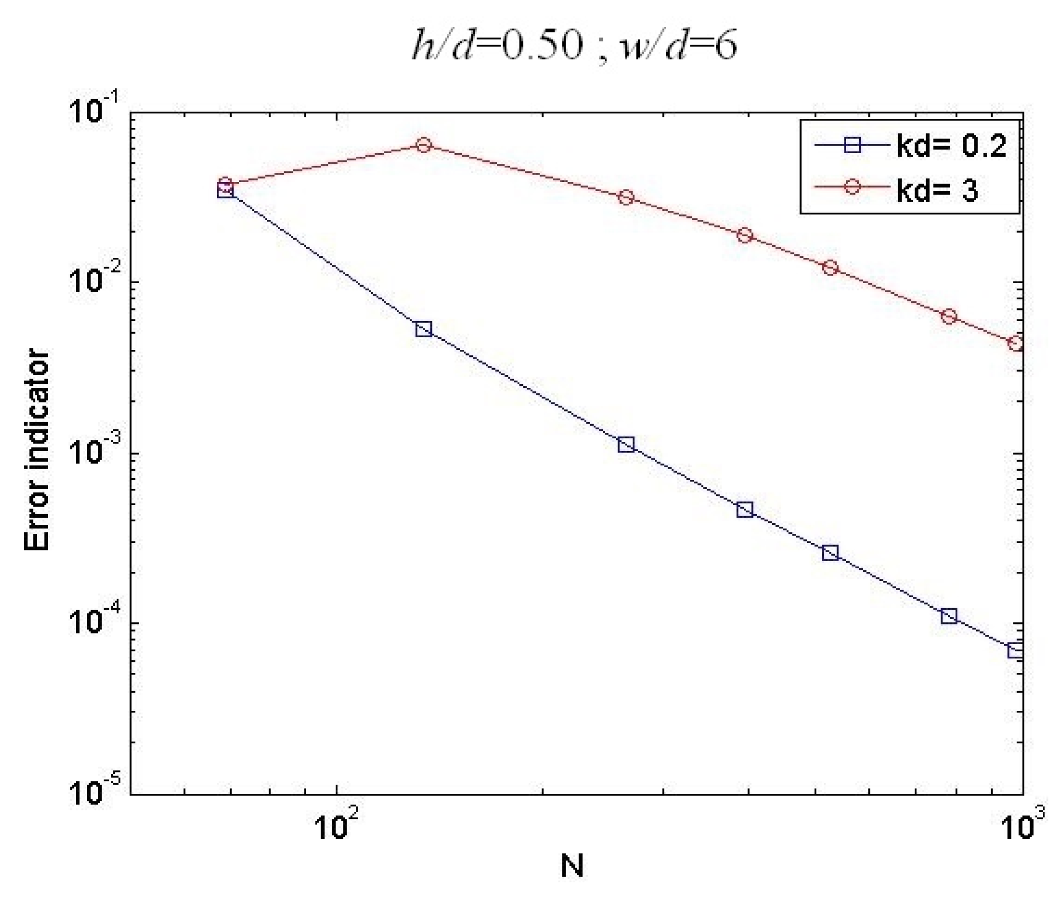
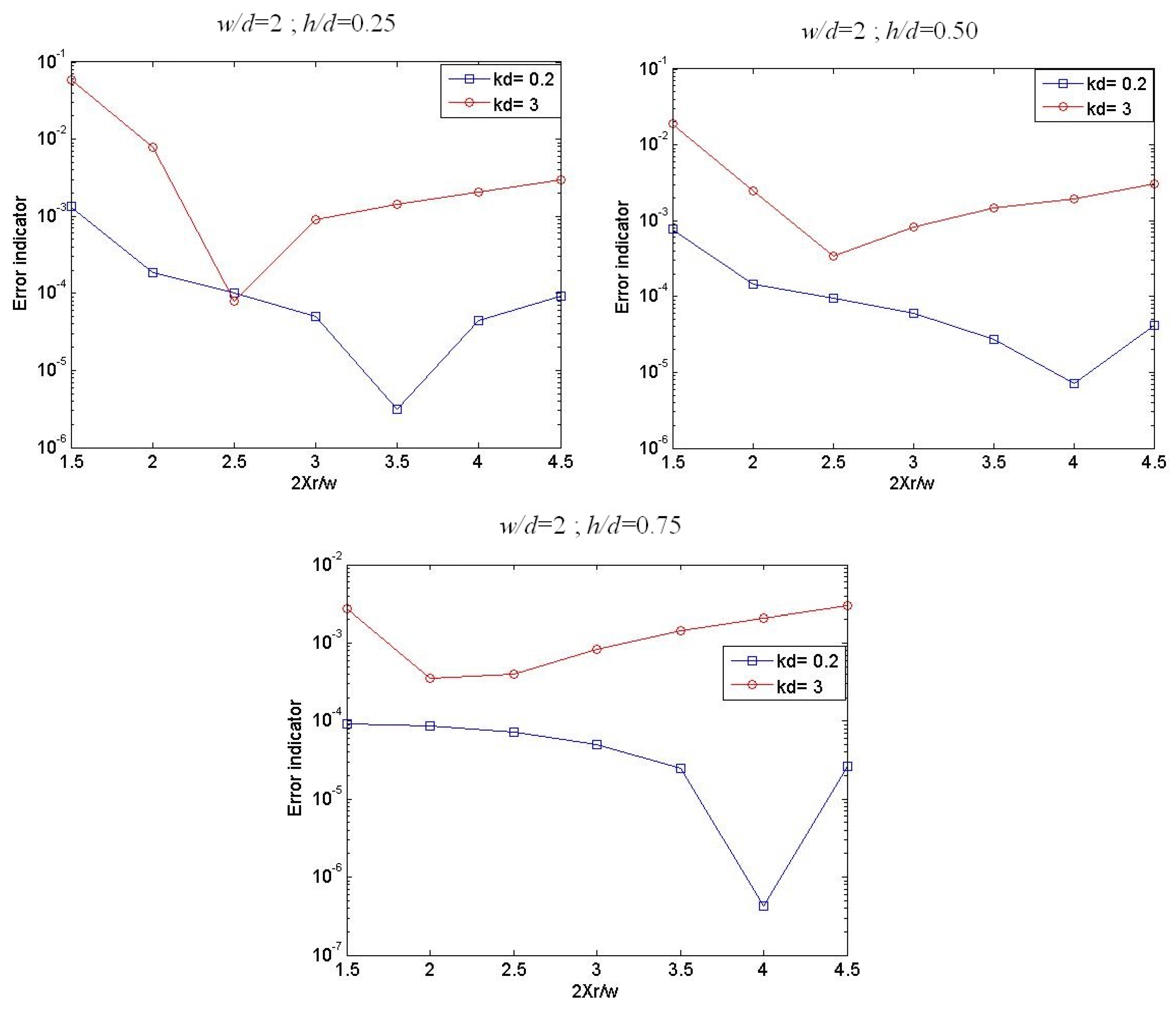
To ensure that the numerical results of the ISBM are acceptable, the sensitivity of the numerical results of the ISBM to the total number of boundary nodes N, and to the positions of the fictitious vertical boundaries, are tested for different immersion ratios (h/d) and for different relative lengths (w/d) of the obstacle. To guarantee tests for small and large values of relative water depth kd, the sensitivity tests are presented for two values of the relative water depths, namely kd = 0.2 and kd = 3.
Energy conservation is expressed as (see [16] for further details), and can be regarded as an error indicator of the numerical solutions. The results are assumed acceptable when errors do not exceed a value of 10−2.
In Figure 4, we examine effects of the total number of boundary nodes N for a fixed relative length w/d = 2 and different immersion ratios, h/d = 0.25, 0.50, 0.75. In Figure 5 the immersion ratio is fixed at h/d = 0.50 and the relative length is varied, w/d = 2, 4, 6. These results show that, for narrow breakwaters (Figure 4), when the immersion ratio h/d is varied, a minimum number of boundary nodes N = 200 is required to ensure that computational errors are small and do not exceed 10−2. However, for wider breakwaters (Figure 5), the total number of boundary nodes is recommended to be at least N = 600 to guarantee that the computational errors remain below 10−2.
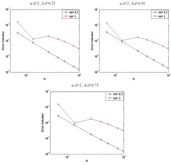
Figure 4.
Error indicator versus the number of boundary nodes for different immersion ratios.
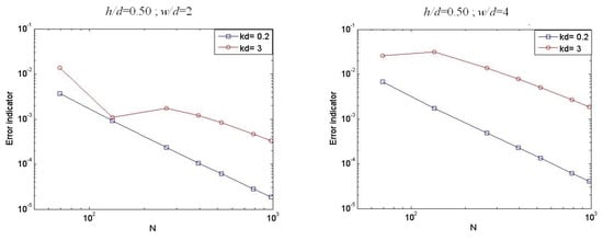
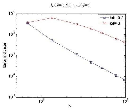
Figure 5.
Error indicator versus the number of boundary nodes for different relative lengths.
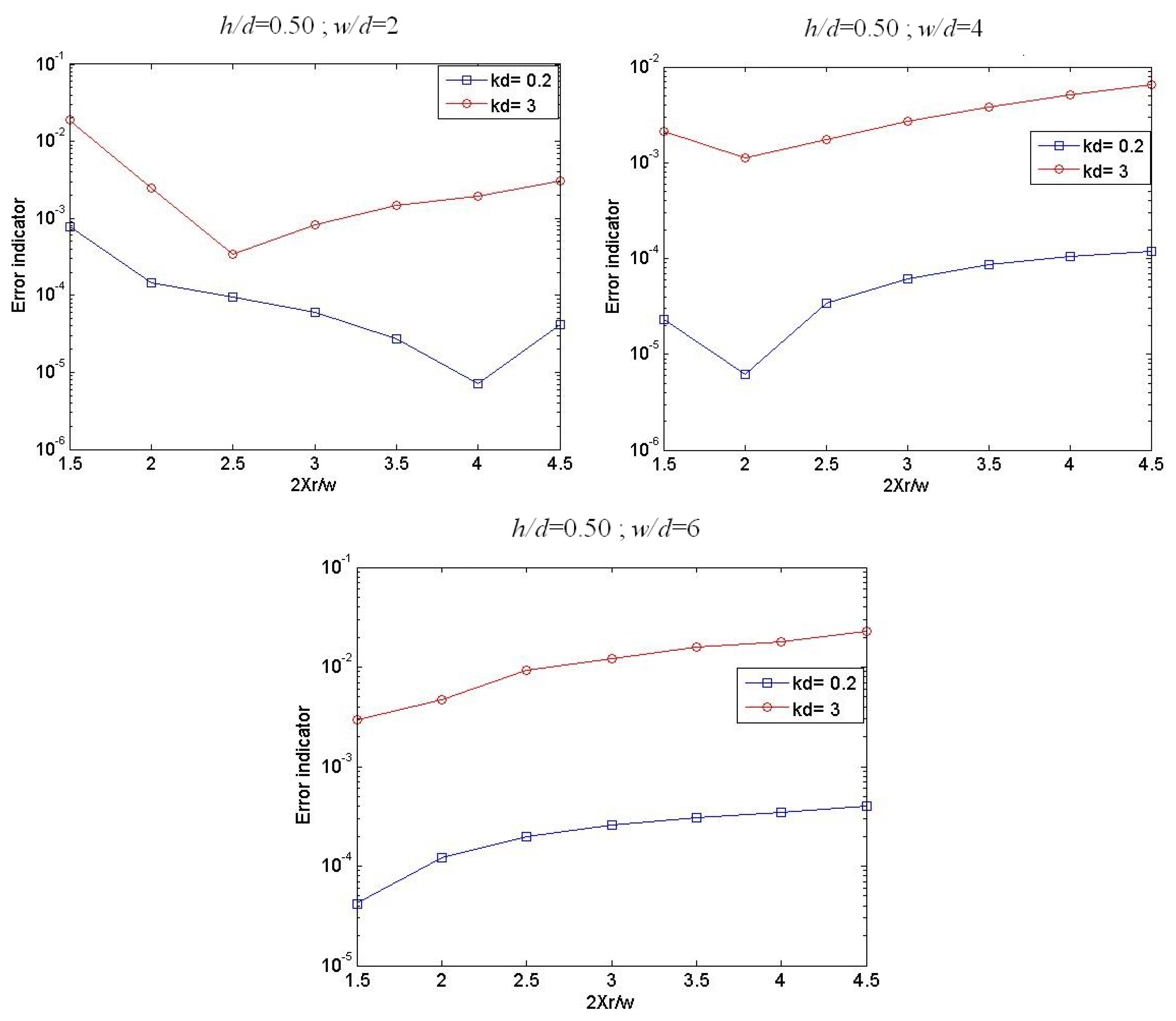
To show the results of the numerical errors with respect to the positions of the fictitious vertical boundaries, we plot the errors against the quantity (relative width of the computational domain). The total number of boundary nodes used in these tests is N = 600. Figure 6 shows the effects of the quantity for a fixed relative length w/d = 2 and different immersion ratios, h/d = 0.25, 0.50, 0.75; whereas, in Figure 7, the immersion ratio is fixed at h/d = 0.50 and the relative length is varied, w/d = 2, 4, 6. The results of Figure 6 for narrow breakwaters show that errors reach minimal values when the quantity is in the range . For these computations, a representative value of = 3 is adopted. Thus, the positions of the fictitious vertical boundaries are fixed, respectively, at . For wider breakwaters, as shown in Figure 7, the results indicate clearly that errors are lowest for . A typical value of = 2 is assumed for these calculations, and therefore the positions of the fictitious vertical boundaries are fixed, respectively, at .
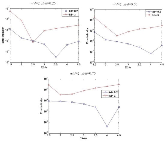
Figure 6.
Error indicator versus the location of vertical fictitious boundaries for different immersion ratios.
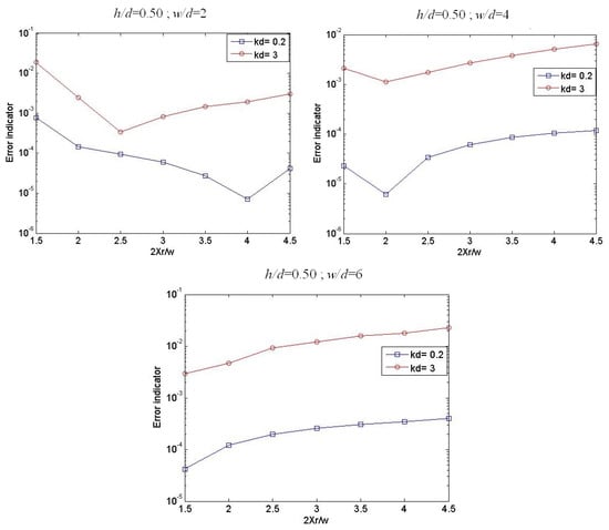
Figure 7.
Error indicator versus the location of vertical fictitious boundaries for different relative lengths.
4.2. Reflection and Transmission Coefficients Analysis
This subsection stands deeply on discussing the reflection and transmission coefficients. Three approaches are used in this work to analyze the reflection and transmission coefficients during the wave interactions with submerged rectangular breakwater. The first approach used is the improved version of the ISBM approach that is already validated in reference [21].
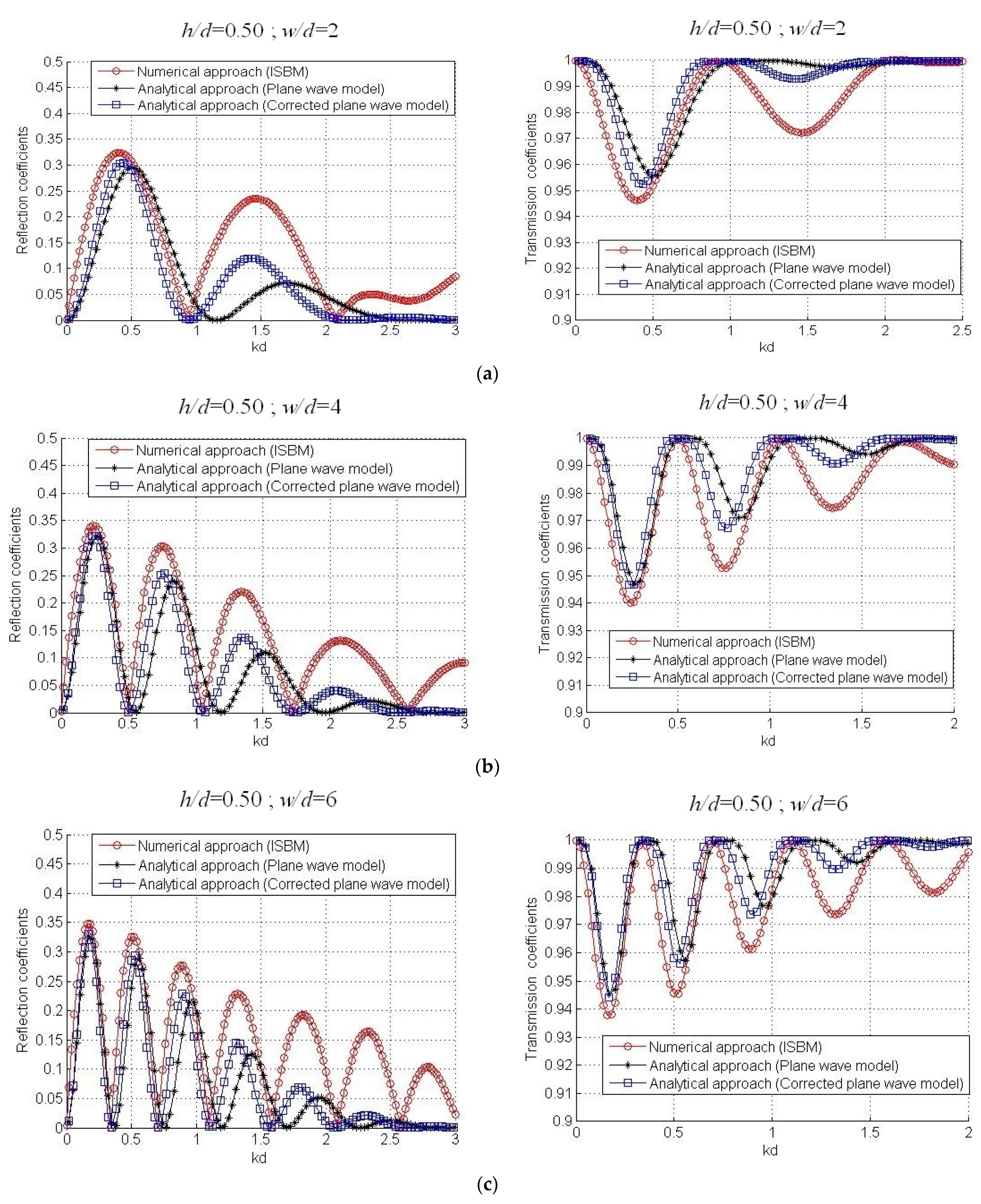
The second approach used is the analytical method within the plane wave model (Appendix A), and the third is the analytical method within the corrected plane wave model. Further, the intention is to figure out the possibility to study the reflection and transmission coefficients using the corrected plane wave model without the introduction of evanescent modes. Firstly, the purpose is to study the validity of reflection and transmission coefficients within the corrected plane wave model, the limitations associated with relative length and the immersion ratio of the submerged rectangular breakwater are studied versus the relative water depth kd, which represents essentially the ratio of water depth to wavelength. Secondly, the goal is to discuss the effect of relative length on reflection and transmission coefficients. Therefore, in Figure 8, the effect of relative length is investigated by fixing the immersion ratio at h/d = 0.50, and varying the relative length into w/d = 2, w/d = 4, and w/d = 6. Thirdly, we aim to study the effect of immersion ratios on reflection and transmission coefficients. Hence, in Figure 9, the effect of immersion ratios is studied by fixing the relative length at w/d = 2, and varying the immersion ratio into h/d = 0.25, h/d = 0.50, and h/d = 0.75.
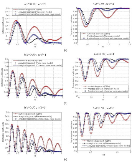
Figure 8.
Variations of reflection and transmission coefficients by fixing the immersion ratio at h/d = 0.50 and varying the relative length: (a) w/d = 2, (b) w/d = 4, and (c) w/d = 6.
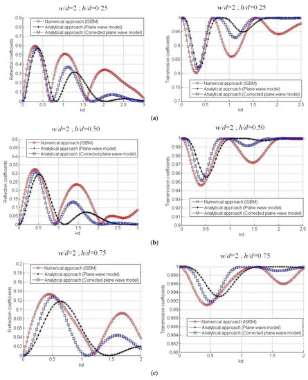
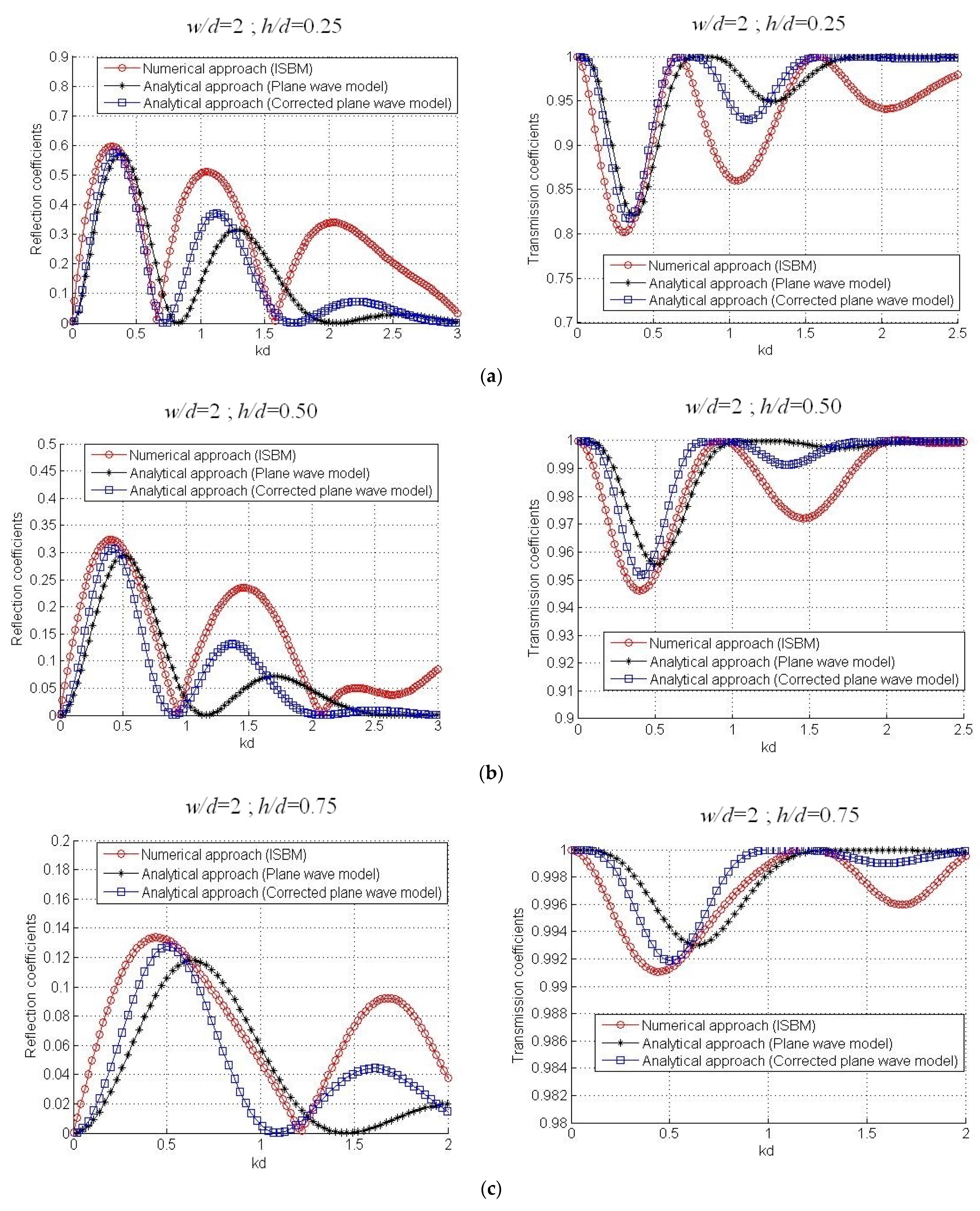
Figure 9.
Variations of reflection and transmission coefficients by fixing the relative length at w/d = 2, and varying values of immersion ratio: (a) h/d = 0.25, (b) h/d = 0.50, (c) h/d = 0.75.
To analyze the reflection and transmission coefficients during the wave interactions with submerged rectangular breakwater, three methods are employed; the first approach is the ISBM, which is already validated in the reference [21]. The second approach used is the analytical method within the plane wave model (Appendix A), and the third is the analytical method within the corrected plane wave model. The plane wave model is corrected by adding 5% to the relative length and subtracting 4% from the immersion ratio. Further, the results of Figure 8 and Figure 9 show that the analytical method within the plane wave model appears slightly far from the ISBM approach, and, as the relative water depth kd increases, the deviation of profiles of the analytical method increases. After several tests, our computational experiments indicate that descriptions of analytical profiles of reflection and transmission coefficients have corrected, and have the same profiles of the ISBM method by adding 5% to the relative length and subtracting 4% from the immersion ratio. Furthermore, the results of the corrected plane wave model are much better than those of the uncorrected plane wave model for all immersion ratios and relative lengths of the obstacle. For these reasons, the corrected plane wave model is strongly recommended. Moreover, the analytical model is based on the use of simple assumptions and simple mathematical manipulations, and the use of the corrected plane wave model presents the advantage of reducing the dimension of algebraic systems treated. In addition, the ISBM method necessitates the mesh generation and the numerical integration. Thus, the analytical model is much easier to use than the ISBM method. Further, the advantages of the corrected plane wave model over the ISBM approach are that it is presented in no condition to the total nodes number, or fictitious vertical boundaries.
On the other hand, the effects of the relative length and immersion ratio on reflection and transmission coefficients, are deeply studied versus the relative water depth kd in Figure 8 and Figure 9. For the sake of clarity, Figure 8, describing the effect of relative length on the variation of reflection and transmission coefficients, shows that the reflection coefficients increase when the relative length increases, whereas the transmission coefficients decrease when the relative length increases. Furthermore, the results show that when the relative length increases, the oscillatory aspect of reflection and transmission coefficients increase, with the appearance of maximum of reflection and transmission coefficients at long wavelengths. Moreover, as the relative water depth increases, the maximum of reflection and transmission coefficients decrease. In addition, Figure 9, describing the effect of immersion ratio on the variation of reflection and transmission coefficients, shows that the reflection coefficients decrease when the immersion ratio increases, whereas the transmission coefficients increase when the immersion ratio decreases.
5. Conclusions and Perspectives
In this research paper, the reflection and transmission coefficients during the interactions of regular wave-rectangular breakwater cited at the bottom are studied using the ISBM approach, the analytical approach within the plane wave model (Appendix A), and the corrected plane wave model. Firstly, to verify the capability of the proposed NWT, the error sensitivity to the total number of boundary nodes, and to positions of fictitious vertical boundaries, for different immersion ratios (h/d) and for different relative length (w/d) of the obstacle, are deeply investigated. Further, the results of this work show that the minimum number of boundary nodes N = 200 is required to ensure an accurate computation solution for narrow breakwaters, and N = 600 for wider breakwaters. Furthermore, to ensure minimal values of errors, the quantity is recommended to be in the range for narrow breakwaters, and for wider breakwaters.
Next, the improved version of the meshless singular boundary method (ISBM), the analytical approach within the plane wave model (Appendix A), and the corrected plane wave model are compared to investigate the capacity of the plane wave and corrected plane wave models to study the reflection and transmission coefficients during interactions of regular wave-rectangular breakwater cited at the bottom of tank. For the sake of details, the plane wave model is efficient for small relative water depths kd; whereas, by correcting the plane wave model by adding 5% to the relative length, and subtracting 4% from the immersion ratio, the corrected plane wave model appears to be in an acceptable agreement with the ISBM approach. Afterwards, the results show that the corrected plane wave model is successful in deeply analyzing the effects of relative length and immersion ratio on reflection and transmission coefficients. Then, it is recommended to use this approach compared to the ISBM method that is conditioned to the nodes number and the position of fictitious vertical boundaries. As perspective, we endeavor to study the wave-current–structure interactions using the Generating-Absorbing Boundary Conditions (GABCs) approach [22] to meticulously study the reflection and transmission coefficients for different aspects of currents.
Author Contributions
Conceptualization, M.L., D.D., C.N., D.N. and K.K.; methodology, M.L., D.D., C.N., D.N. and K.K.; software, M.L., D.D., C.N., D.N. and K.K.; validation M.L., D.D., C.N., D.N. and K.K.; formal analysis M.L., D.D., C.N., D.N. and K.K.; investigation, M.L., D.D., C.N., D.N. and K.K.; resources, M.L., D.D., C.N., D.N. and K.K.; writing—original draft preparation, M.L., D.D., C.N., D.N. and K.K.; writing—review and editing, M.L., D.D., C.N., D.N. and K.K.; visualization, M.L., D.D., C.N., D.N. and K.K.; supervision, M.L., D.D., C.N., D.N. and K.K.; project administration, M.L., D.D., C.N., D.N. and K.K.; funding acquisition, M.L., D.D., C.N., D.N. and K.K. All authors have read and agreed to the published version of the manuscript.
Funding
The work of DD has been supported by the French National Research Agency, through the Investments for Future Program (ref. ANR-18-EURE-0016—Solar Academy).
Institutional Review Board Statement
Not applicable.
Informed Consent Statement
Not applicable.
Data Availability Statement
Not applicable.
Acknowledgments
The Authors would like to express their gratitude to the Referees who helped us to improve our manuscript quality.
Conflicts of Interest
The authors declare no conflict of interest.
Nomenclature
| The amplitude of the incident wave | |
| T | The period |
| R | The reflection coefficient |
| The transmission coefficient | |
| d | The water depth |
| h | The water depth above the obstacle |
| w | The length of the obstacle |
| h/d | The immersion ratio |
| w/d | The relative length |
| The wave number that verifies the dispersion relation | |
| The wave number above of the obstacle that verifies the dispersion relation |
Appendix A
In this section, the objective is to present an analytical approach to calculate the reflection and transmission coefficients during the interaction of regular wave-rectangular obstacle cited at the bottom of tank. Within the plane wave approach, Dingemans [23] has already presented the reflection and transmission coefficients based on matching conditions approach where the continuity of the velocity potential as long with the horizontal velocity over the subdomains is neglected. In this paper, we subdivide the domain of study (cf. Figure A1) into three sub-domains (, , ), where the continuity of velocity potential and horizontal velocity are expressed at edges of the obstacle to determine the reflection and transmission coefficients. By expressing the connection conditions at edges of the obstacle, our approach appears to be simpler and mre accurate than presented by Dingemans [23].
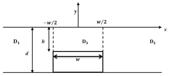
Figure A1.
Domain of study.
Figure A1.
Domain of study.
At each subdomain the velocity potential is expressed as:
- -
- at the subdomain
- -
- at the subdomain
- -
- at the subdomain
The continuity of the velocity potential and horizontal velocity are expressed at two positions x = and position x = as:
- At the position x =
- At the position x=after expressing the connection conditions at the positions x = and x = , we obtain a linear algebraic system aswhere:by combining the system of Equation (8), we obtain
Then, by injecting the expressions (12) and (13) in the second and fourth equation of the system (8), we obtain
with , more explicitly,
Then, we obtain a matrix system as
The resolution of the matrix system makes it possible to obtain the expression of the reflection and transmission coefficients as
where:
Appendix B
The potentials at the fictitious boundaries and , defined at and respectively, are written as:
where , and are the incident, reflected and transmitted wave amplitudes respectively.
The reflection and transmission coefficients R and are defined as:
Substituting the relations given by Equation (A24) into Equations (A22) and (A23) we get:
Now defining the following expressions as:
and substituting into Equations (A25) and (A26) , we finally achieve the final expressions of the inflow and outflow potentials:
After calculating the potentials and from the ISBM, they are matched to those of Equations (A28) and (A29) at and respectively, then the unknown coefficients and are evaluated as follows. When Equations (A28) and (A29) are evaluated at and they become:
We can now multiply both sides of Equations (A30) and (A31) by to give:
Integrating y in Equations (A32) and (A33) between 0 and d, and after manipulating the resulting algebraic expressions, we get:
where .
Referring to Equation (A27) , the reflection and transmission coefficients are Finally calculated as:
References
- Dean, W.R. On the reflexion of surface waves by a submerged plane barrier. In Mathematical Proceedings of the Cambridge Philosophical Society; Cambridge University Press: Cambridge, UK, 1945; Volume 41, pp. 231–238. [Google Scholar]
- Takano, K. Effets d’un obstacle parallélépipédique sur la propagation de la houle. Houille Blanche 1960, 3, 247–267. [Google Scholar] [CrossRef] [Green Version]
- Patarapanich, M. Forces and moment on a horizontal plate due to wave scattering. Coast. Eng. 1984, 83, 279–301. [Google Scholar] [CrossRef]
- Liu, P.L.F.; Wu, J. Wave transmission through submerged apertures. J. Waterw. Port Coast. Ocean Eng. 1987, 113, 660–671. [Google Scholar] [CrossRef]
- Stamos, D.J.; Hajj, M.R.; Telionis, D.P. Performance of hemi-cylindrical and rectangular submerged breakwaters. Ocean Eng. 2003, 30, 813–828. [Google Scholar] [CrossRef]
- Molin, B.; Kimmoun., O.; Liu., Y.; Remy., F.; Bingham, H.B. Experimental and numerical study of the wave run-up along a vertical plate. J. Fluid Mech. 2010, 654, 363–386. [Google Scholar] [CrossRef]
- Liu, Y.; Li, H.J.; Zhu, L. Bragg reflection of water waves by multiple submerged semi-circular breakwaters. Appl. Ocean Res. 2016, 11, 67–78. [Google Scholar] [CrossRef]
- Scyphers, S.B.; Powers, S.P.; Heck, K.L. Ecological Value of Submerged Breakwaters for Habitat Enhancement on a Residential Scale. Environ. Manag. 2015, 55, 383–391. [Google Scholar] [CrossRef] [PubMed]
- Mei, C.; Black, J. Scattering of surface waves by rectangular obstacles in waters of finite depth. J. Fluid Mech. 1969, 38, 499–511. [Google Scholar] [CrossRef]
- Massel, S. Harmonic generation by waves propagating over a submerged step. Coast. Eng. 1983, 7, 357–380. [Google Scholar] [CrossRef]
- Driscoll, A.; Dalrymple, R.; Grilli, S. Harmonic generation and transmission past a submerged rectangular obstacle. Coast. Eng. 1992, 1142–1152. [Google Scholar] [CrossRef]
- Szmidt, K. Finite difference analysis of surface wave scattering by underwater rectangular obstacles. Arch. Hydro-Eng. Environ. Mech. 2010, 57, 179–198. [Google Scholar]
- Chen, W.; Gu, Y. An improved formulation of singular boundary method. Adv. Appl. Math. Mech. 2012, 4, 543–558. [Google Scholar] [CrossRef]
- Gu, Y.; Chen, W.; Zhang, J.Y. Investigation on near-boundary solutions by singular boundary method. Eng. Anal. Bound. Elem. 2012, 36, 1173–1182. [Google Scholar] [CrossRef]
- Gu, Y.; Chen, W. Infinite domain potential problems by a new formulation of singular boundary method. Appl. Math. Model. 2013, 37, 1638–1651. [Google Scholar] [CrossRef]
- Chioukh, N.; Çevik, E.; Yüksel, Y. Reflection and transmission of regular waves from/through single and double perforated thin walls. China Ocean Eng. 2017, 31, 466–475. [Google Scholar] [CrossRef]
- Bakhti, Y.; Chioukh, N.; Hamoudi, B.; Boukhari, M. A multi-domain boundary element method to analyze the reflection and transmission of oblique waves from double porous thin walls. J. Mar. Sci. Appl. 2017, 16, 276–285. [Google Scholar] [CrossRef]
- Yueh, C.Y.; Chuang, S.H. A boundary element model for a partially piston-type porous wave energy converter in gravity waves. Eng. Anal. Bound. Elem. 2012, 36, 658–664. [Google Scholar] [CrossRef]
- Brebbia, C.A.; Dominguez, J. Boundary Elements: An Introductory Course. In Computational Mechanics Publications; WIT Press: Southampton, UK; Boston, MA, USA, 1992. [Google Scholar]
- Gu, Y.; Chen, W. Recent advances in singular boundary method for ultra-thin structural problems. In Boundary Elements and Other Mesh Reduction Methods XXXVI; WIT Transactions on Modelling and Simulation: Southampton, UK; Boston, MA, USA, 2014; Volume 56, pp. 233–243. [Google Scholar]
- Senouci, F.; Chioukh, N.; Dris, M.E.A. Performance Evaluation of Bottom-Standing Submerged Breakwaters in Regular Waves Using the Meshless Singular Boundary Method. J. Ocean Univ. China 2019, 18, 823–833. [Google Scholar] [CrossRef]
- Loukili, M.; Dutykh, D.; Kotrasova, K.; Ning, D. Numerical Stability Investigations of the Method of Fundamental Solutions Applied to Wave-Current Interactions Using Generating-Absorbing Boundary Conditions. Symmetry 2021, 13, 1153. [Google Scholar] [CrossRef]
- Dingemans, M. Water Wave Propagation Over Uneven Bottoms. Adv. Ser. Ocean Eng. 1997, 13, 1–1016. [Google Scholar] [CrossRef]

Publisher’s Note: MDPI stays neutral with regard to jurisdictional claims in published maps and institutional affiliations. |
© 2021 by the authors. Licensee MDPI, Basel, Switzerland. This article is an open access article distributed under the terms and conditions of the Creative Commons Attribution (CC BY) license (https://creativecommons.org/licenses/by/4.0/).