Article

A Computer Aided Approach for River Styles—Inspired Characterization of Large Basins: A Structured Procedure and Support Tools

by
Andrea Nardini
1,2,
Santiago Yépez
3,4,* and
Maria Dolores Bejarano
5
1
Fundación CREACUA (Centro para la Recuperación de Ecosistemas ACUAticos), 440001 Riohacha, La Guajira, Colombia
2
PhD Program in Advanced Forestry Engineering, Escuela de Montes, Universidad Politécnica de Madrid (UPM), 28040 Madrid, Spain
3
Departamento Manejo de Bosques y Medio Ambiente, Facultad de Ciencias Forestales, Universidad de Concepción (UdeC), Concepción 407374, Chile
4
Laboratorio de Geotecnologías y Modelamiento de Recursos Naturales (LGM), Universidad de Concepción (UdeC), Concepción 407374, Chile
5
Escuela de Montes, Universidad Politécnica de Madrid (UPM), 28040 Madrid, Spain
*
Author to whom correspondence should be addressed.
Geosciences 2020, 10(6), 231; https://doi.org/10.3390/geosciences10060231
Submission received: 3 March 2020 / Revised: 26 May 2020 / Accepted: 10 June 2020 / Published: 15 June 2020
(This article belongs to the Special Issue Numerical Modeling of Surface Processes)

Abstract

:
This paper presents a systematic procedure for developing a characterization and classification of river reaches inspired by the River Styles Framework, through which insight can be gained about the understanding of river behavior. Our procedure takes advantage of several computer based “tools”, i.e., algorithms implemented in software packages of various types, from “simple” Excel sheets to sophisticated algorithms in Python language, in general all supported by Geographic Information Systems (GIS). The main potentially useful, existing tools for this specific aim are discussed here, revealing their strengths and weaknesses. New, complementary or alternative tools that have been developed in the project feeding this paper are presented, which can contribute to the scientific community and stakeholders of the topic. The main result of our research is a structured and practical guide (a ToolBox Manual) that can support practitioners and researchers wishing to characterize and classify large rivers, based on the River Styles Framework. The main contribution is that this set of ideas, solutions, and tools, makes this type of exercise significantly more transparent and at the same time much less subjective. Moreover, the procedure is applicable to large systems and does not require more information than that generally available also in developing or emerging countries.

1. Introduction

Today, remote sensing offers unprecedented opportunities to analyze rivers, particularly in large basins. Piégay et al. [1] present a very complete, articulated, and up-to-date panorama of the techniques, recent experiences, and emerging research challenges that use or are related to remotely sensed data for geomorphic river characterization and management and, particularly, to investigate past, present, and future fluvial corridor conditions and processes. Most of these very refined and complex techniques and experiences relate to the identification of geomorphic units (e.g., main channel, bars, islands, etc.) or the measure of some features (e.g., topographic, vegetation structure); others are focused on the search for (cause–effect) relationships between natural or anthropogenic factors and the geomorphic response of the river, including its time evolution (e.g., widening, narrowing; incision/aggradation); still others are dedicated to monitoring river behavior, either through periodic, systematically repeated surveys or real time observation. It can be argued that there is no better way to describe how a river actually works than observing its actual dynamic behavior along a significant time span and across different spatial scales. However, a basic, fundamental understanding can be obtained by looking at the main, present characteristics of the river at different scales, simultaneously, and recognizing how different assemblages of geomorphic units occur in relation to forcing factors (“controls”) such as geology, topography, climate, and human interventions. This essentially static analysis, when integrated with information concerning the historical evolution of a river, provides a very sound basis for understanding its character and behavior from a geomorphological perspective. This is the essence of the River Styles Framework (RS onwards) developed by Brierley and Fryirs [2]. Of course, information generated with this framework can be corroborated, refined, and integrated with further, more advanced and complex analyses, where tools like those presented by Piégay et al. [1] can be extremely valuable.
The River Styles approach, however, requires a quite demanding analysis effort, particularly when dealing with large basins. In addition, it incorporates a high dose of subjectivity as it involves several expert-based judgment inputs. This latter point is a delicate one, as computer-based tools and remotely sensed data evolve and somehow challenge the role of the human expert (geomorphologist), which is hence being continuously re-discussed [3,4].
The aim of this paper is widening the audience of river practitioners, managers, and researchers that would like to apply the RS Framework as potential beneficiaries, but which may be reluctant to do because of the practical difficulties that are typically encountered, particularly when trying to apply it to large river basins. We contribute to this aim, on the one hand, by defining a more structured, objective, and straightforward procedure, in which the role of the geomorphology experts is more clearly identified and circumscribed, and, on the other hand, by suggesting concrete computer-based tools options to support the required tasks and, even, automate a large part of the exercise. While Fryirs et al. [4] offer a broad spectrum view of available tools and their possible role in the RS analysis (and more), which is certainly stimulating, we concentrate on the practitioners’ point of view, as we assume they are keen to find as simple and concrete guidelines as possible, to actually perform the multiple tasks.
It is important to point out that the RS Framework involves a number of stages and steps, of which we only consider here “Stage I, steps 1 and 2”, i.e., the “characterization-classification” exercise; in what follows, we refer to these as the “RS analysis”. The findings presented in this paper are products of a project conducted by some of us for The Nature Conservancy, in Colombia; we are referring to it in the following as the “GeoMagda project”. It is worth noting that these findings have been articulated in a number of more or less simultaneous articles and, as such, unavoidably we need to refer to them.
Several important research groups are contributing to the plethora of methodologies and tools aiming at supporting geomorphic river analysis. With no pretention of exhaustiveness, we identify the following main ones:
The Riverscapes consortium https://www.riverscapes.xyz/, a collaboration between fluvial researchers in the United States of America, United Kingdom, New Zealand, Australia, Italy, France, and Spain, particularly with its ToolBox RCAT (http://rcat.riverscapes.xyz/), which includes: the Valley Bottom Extraction Tool (V-BET), the Riparian Vegetation Departure (RVD) tool, the Riparian Condition Assessment (RCA) tool, and the Riparian Recovery Potential (RRP) tool.
The Valley Bottom Confinement Tool (VBCT), developed and based on studies by Fryirs et al. [4,5] and O’Brien et al. [6] (http://confinement.riverscapes.xyz/).
The TerEx ToolBox (terrace and floodplain mapping), based on the work of Clubb et al. [7] and Stout and Belmont [8] (https://qcnr.usu.edu/labs/belmont_lab/resources).
The Fluvial Corridor ToolBox (FCT), by the group led by Hervé Piégay at the University of Lyon (France); currently, they are developing a version within the QGIS 3.x interface compiling scripts written in Python (https://github.com/tramebleue/fct).
The River Meandering Migration Software (RVRMeander; http://www.rvrmeander.org/) of the University of Illinois, University of Pittsburgh, and USDA(U.S. Department Of Agriculture), with applications in particular to the Amazon River by Jorge Abad.
The Geomorphic Unit Tool (GUT), which delineates instream geomorphic units (GUs) from topography using a three-tiered hierarchical classification adapted from Wheaton et al. [9] (http://gut.riverscapes.xyz/).
To this we can add the REFORM (REstoring rivers FOR effective catchment Management) project [10] presenting a host of methods concerning the interpretation of remote sensing data (e.g., [3,11,12,13,14,15]), as well as the already mentioned Fryirs et al. [4] and Piégay et al. [1].
The use of most of these tools, however, is typically quite complicated and delicate. They generally require a Python installation that often generates difficulties. They always require a human refinement of their outputs, which introduces a hidden degree of arbitrariness. Some (such as RCAT) are explicitly designed to be fed with the standard information available in the USA. Others (e.g. the RVRMeander) are explicitly aimed at meandering rivers. Several are in principle interchangeable because they address the same task, although with some differences. No single one, however, embeds all of the functionalities needed to carry out a River Styles analysis. Finally, most of them are simply not applicable in cases characterized by scarce information, including low resolution geographic data (particularly Digital Elevation Models-DEM).
The most applicable tool to support RS analysis, amongst those listed, is certainly the Fluvial Corridor ToolBox. However, its actual usefulness for performing RS analysis is definitely much reduced, for several reasons, with respect to the potentialities that were originally been announced in the FCT Project. On the one hand, the sequence of sub-tools that appears when installing it (within ArcGIS) does not correspond to the actual sequence of use, a quite confusing fact. Additionally, several steps and functionalities are not relevant for RS analysis and thus must be skipped, while, conversely, other key functionalities are not supported (e.g., confinement or RS classification). Another issue is that the computation of sinuosity within the FCT is based on the polyline connecting inflection points of the active bed centerline; in some cases, this may result in a polyline external to the valley bottom (VB), which should not happen. Finally, the key Hubert test for identifying homogenous reaches does not work with non-cardinal indicators, which are nonetheless often involved in RS analysis. Moreover, several “tricks” need to be known; to a novel user, many of these may appear to be unsolvable snags, leading him/her to quit.
This paper addresses mainly the community of practitioners by providing a guide through the different elaborations needed when conducting a RS exercise. Its main contribution in this sense is providing a procedure that allows to link all the required steps in a structured, operational form. In such a way, on the one side, the role for expert judgment becomes better defined, so that the outputs are structurally more objective; on the other side, the procedure makes RS characterization–classification viable also for large rivers, by taking advantage of computer-aided tools. The paper may also be of interest to the scientific community, as it addresses some challenging conceptual problems concerning the holistic synthesis of reductionist information that lie at the core of the automated analysis of complex information. We are aware, anyway, that the main added value of this paper can be appreciated by those who know and have adopted (or would like to adopt) the River Styles Framework.
In what follows, we first present the essence of the proposed procedure (details are provided in Appendix A); then, some of the newly developed tools are presented, together with demonstrative applications to the Magdalena River case study (Colombia); finally, conclusions are drawn.

2. Systematizing a River Styles Inspired Characterization–Classification Exercise

Figure 1 presents a summary view of the steps we consider necessary to conduct a RS analysis (Stage I, steps 1 and 2 of the RS Framework), while Table A1 in Appendix A presents a much more detailed picture. For each step, we indicate the tool/procedure suggested; in some cases, several options are proposed, depending on the original information available. The list does not claim to be exhaustive (see also [1,3,4,11,12,13,14,15] for additional options); rather, its purpose is to give an idea of the complexity of a full RS analysis exercise, and to locate within the process the additional tools we explicitly developed, which are described in detail in the ToolBox Manual [16].
Expert judgment is involved on one hand in defining criteria to be adopted within the various steps (e.g., defining the Procedural Tree; or defining how to distinguish a planform type from another) and, on the other, after the procedure has been applied, in interpreting river behavior. This exercise must be accompanied by an analysis of the river’s historical behavior and recent adjustments (not included herein).
As anticipated, the added value of this procedure can be fully appreciated by those who know and have used (or would like to adopt) the River Styles Framework. The innovations are evident only when analyzing the details, but consist mainly of:
(a)
Modifying the Procedural Tree, by “locating first what weighs more”, in such a way that a hierarchical classification can be obtained that can manage all sub-types generated in particular by the assemblage of the different geomorphological units (which can give rise to a large number of sub styles).
(b)
Identifying objectively the (variable length) reaches according to the spatial intersection of only the set of intensive-type attributes of the Procedural Tree (i.e., those not depending on the extension of the length of the considered segment) and assessing all the extensive-type attributes as spatial statistics over such reaches. This idea is further explained in [16,17,18].
(c)
Relying on a spatial database (called “skeleton”) obtained by segmenting the valley bottom in sub-segments along its axis, and determining a value for each relevant attribute in each sub-segment.
(d)
Specifying a set of tools that ensure the ability to also deal with large river systems. The proposed tools (Appendix A) are a particular choice out of a virtually infinite (or at least quite large) number of alternatives; but having defined at least a tool set that does cover all the demanding steps (elaborations of extensive information and computational steps) brings in an added value as, without them, several snags might prevent a candidate user from applying the RS approach.
(e)
Proposing a sequence of operations that covers the whole exercise, ensuring a linkage amongst steps and avoiding redundancies.
Concerning aspect (d), the ToolBox Manual developed within the GeoMagda project provides quite detailed instructions on how to solve a number of difficulties; this might be superfluous to the trained GIS expert, but precious to a broader arena of users. It is worth stressing that the tools we propose require just a basic expertise in computer use, particularly GIS and Excel; this has a negative facet, as advantage is not taken of more powerful possibilities, but it also has a positive facet, as broadens the arena of candidate users and to improvements.
It is worth noting that the first main product of this paper is Table A1 in Appendix A, which presents the full procedure we propose.
In the following section, we address just three “tools” amongst those developed and included in Table A1, in order to give an idea of the type of contribution this paper (and the underlying GeoMagda project) brings in. To illustrate some of the concepts and type of results we utilize the Magdalena case study developed in [16,17]. What follows should not be interpreted, however, as the application to the Magdalena of the full procedure; rather, the focus here is using the Magdalena data just to illustrate how these “tools” work (any other data would serve this purpose). A synthesis of the Magdalena case study is available in Nardini et al. [17], where we show the essential outputs obtainable by applying the procedure described herein; details can be found in [16,17]. We warmly suggest that this paper be read together with the case study (and also with Nardini et al. [18] when it be published) because they are indeed highly complementary. From a methodological point of view, Nardini et al. [17] present the essential contents of a River Styles characterization–classification exercise, while here we present the organized collection of technical steps involved.
It is important that the reader not get lost in the following technicalities: the essential message we would like to convey is that the procedure we have developed addresses several points similar to those discussed below, proposing conceptual and operational solutions to overcome any issues, while simultaneously ensuring that all steps are linked in a harmonic fashion.

3. New Tools/Procedures

3.1. Confinement

Confinement, as adopted in the RS Framework, expresses the extent to which the river abuts either valley bottom (VB) margin. It is a very meaningful attribute because this condition strongly characterizes the dynamic behavior of the river itself. It should not be confused with “entrenchment”, i.e., the ratio between active channel width and VB width [19].
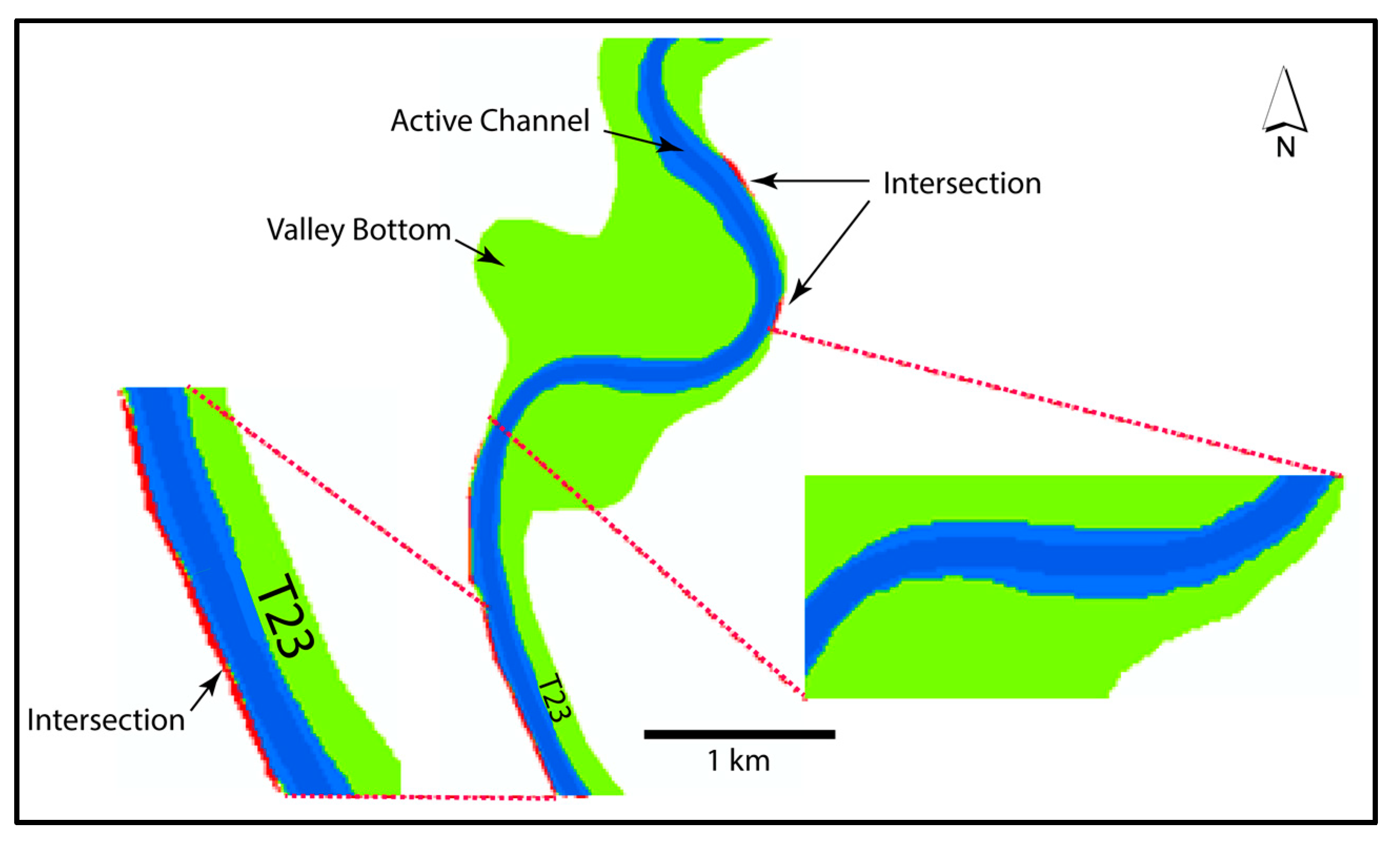
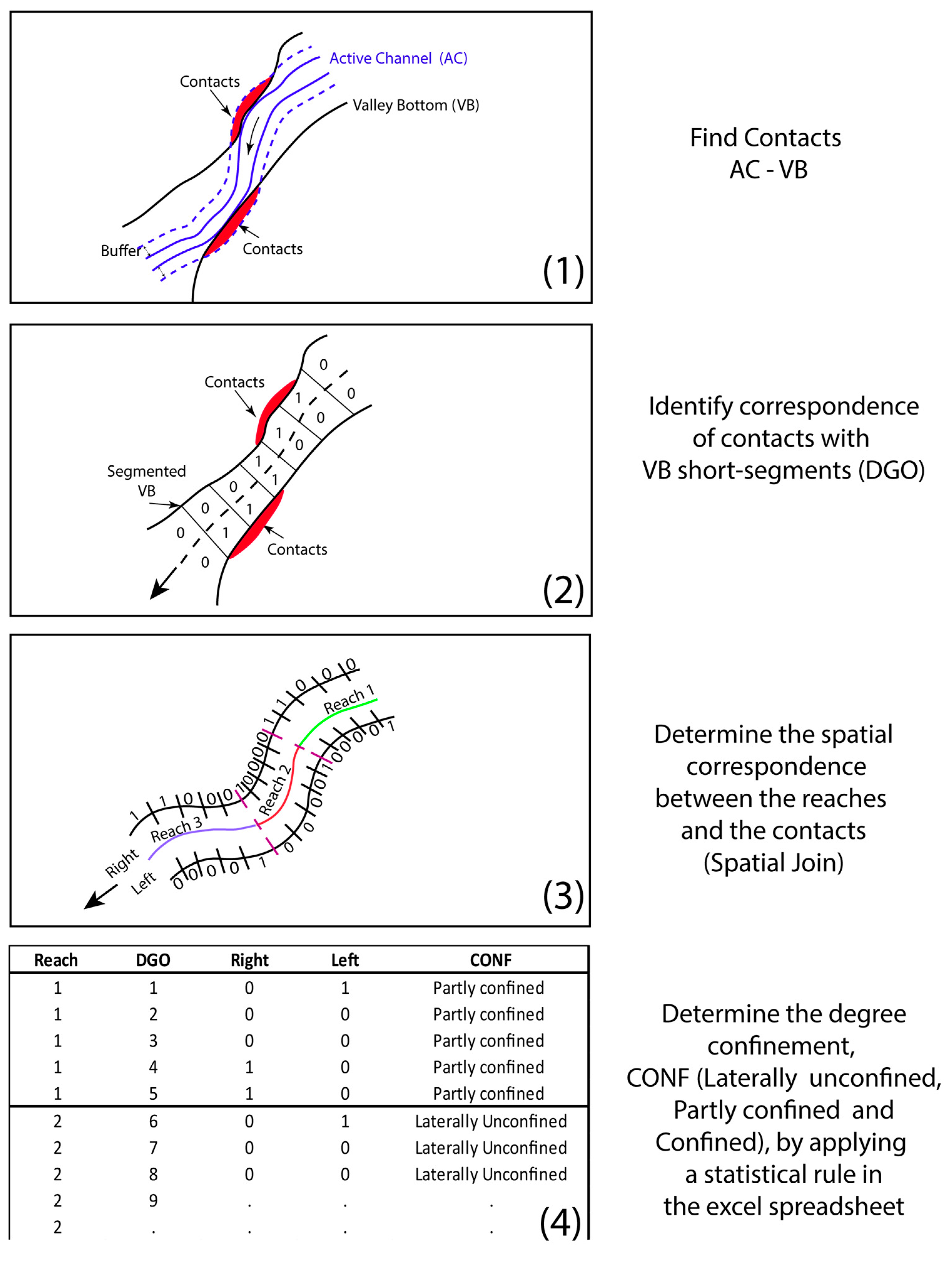
To assess confinement, the objective, relevant base information is the set of contacts between the active channel (or, more generally, the envelope of active channels) and the VB margins. However, to meaningfully characterize a reach in terms of confinement, one has to rely on a statistical, categorical indicator (% of either bank’s contact lengths over the corresponding axis length) according to some given convention (according to Brierley and Fryirs, [2]: laterally “unconfined” when total contact is less than 10%; “confined”, when is over 85%; “partly confined”, when in between) over a given reach (product of a segmentation). Indeed, the result strongly depends on the segmentation adopted, as shown in Figure 2.
The main novelty of the algorithm we propose to define confinement lies in determining it after reaches are defined. In fact, this position overcomes an intrinsic logical problem of the traditional approach: in the RS framework, reaches displaying a recognizable and meaningful pattern are identified as the output of a process based on assessing the set of attributes included within the RS Procedural Tree; but the first of such attributes is indeed confinement, which requires—as we have shown—that segments (i.e., reaches) be pre-defined.
Additionally, our algorithm determines an explicit statistical confinement indicator as well as another important attribute which is the cause of confinement, once the polylines of the VB margins separated in categories (i.e., valley margin, planform, and infrastructure) are provided. Furthermore, it brings a clear advantage from a practical point of view: it is accessible to anyone able to use ArcGIS (or QGIS) and Excel.
Finally, as confinement is determined for any given segmentation, it is possible and meaningful to provide the output at different scales; particularly:
(i)
reaches (as usually done in the RS);
(ii)
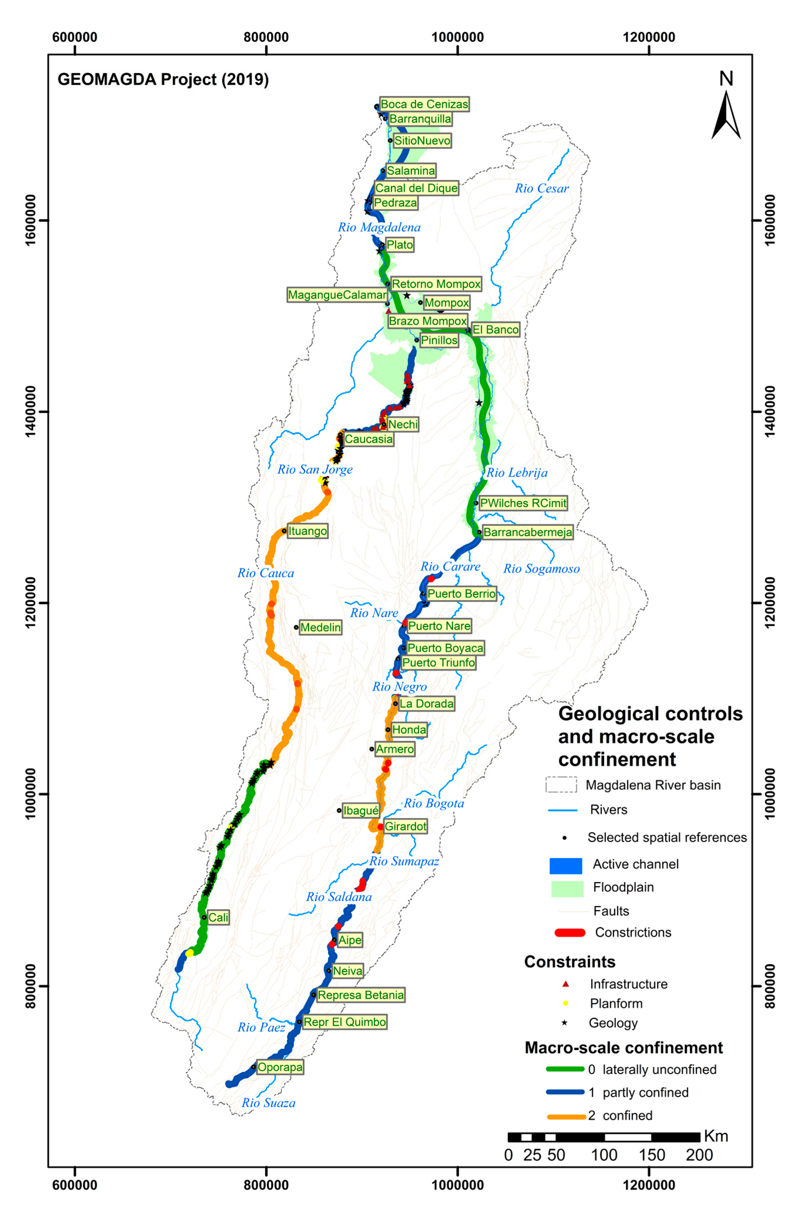
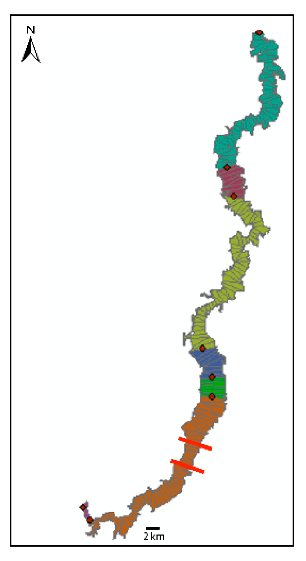
basin scale (macro): indeed, it is possible to adopt a very simple and effective criterion to identify macro segments, e.g., where a significant change of VB width (V) occurs (a fact that can be detected by the Hubert Test in the FCT or simply...visually) and the resulting macro confinement is very meaningful (Figure 3).
As O’Brien et al. [6] have already presented an algorithm, with a corresponding GIS Python software tool, to determine the confinement indicator within the RS context, it is important to recall it and point out the differences with our approach. That algorithm goes as follows:
it determines the contacts—both margins—between active channel and “inflated” (buffer) VB margin through a GIS intersection;
these contacts are projected onto the reference axis with a binary value (0 for no contact; 1 for contact at either bank);
the axis is discretized in “short-segments” (identified by k) of a pre-fixed length;
the algorithm goes on by computing locally (for each slice) the statistical indicator c(k) as the total length of the projected contacts (either banks) falling in it, over the segment length;
finally, it assumes that when the indicator c(k) is 0.50 < c(k) < 0.85 the cause of confinement is the valley margin, while when it is 0.10 < c(k) < 0.50 the cause is a planform geomorphic unit.
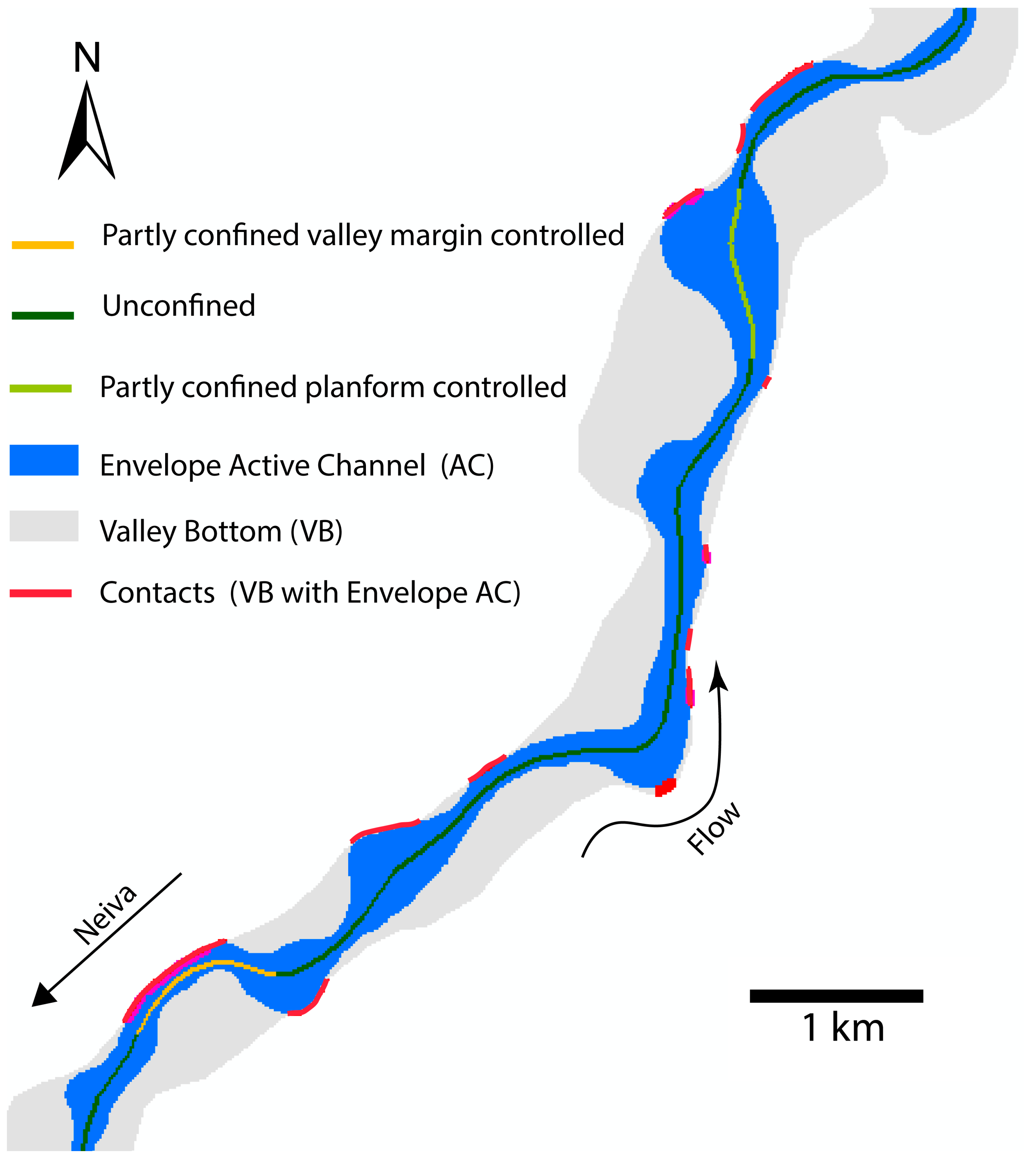
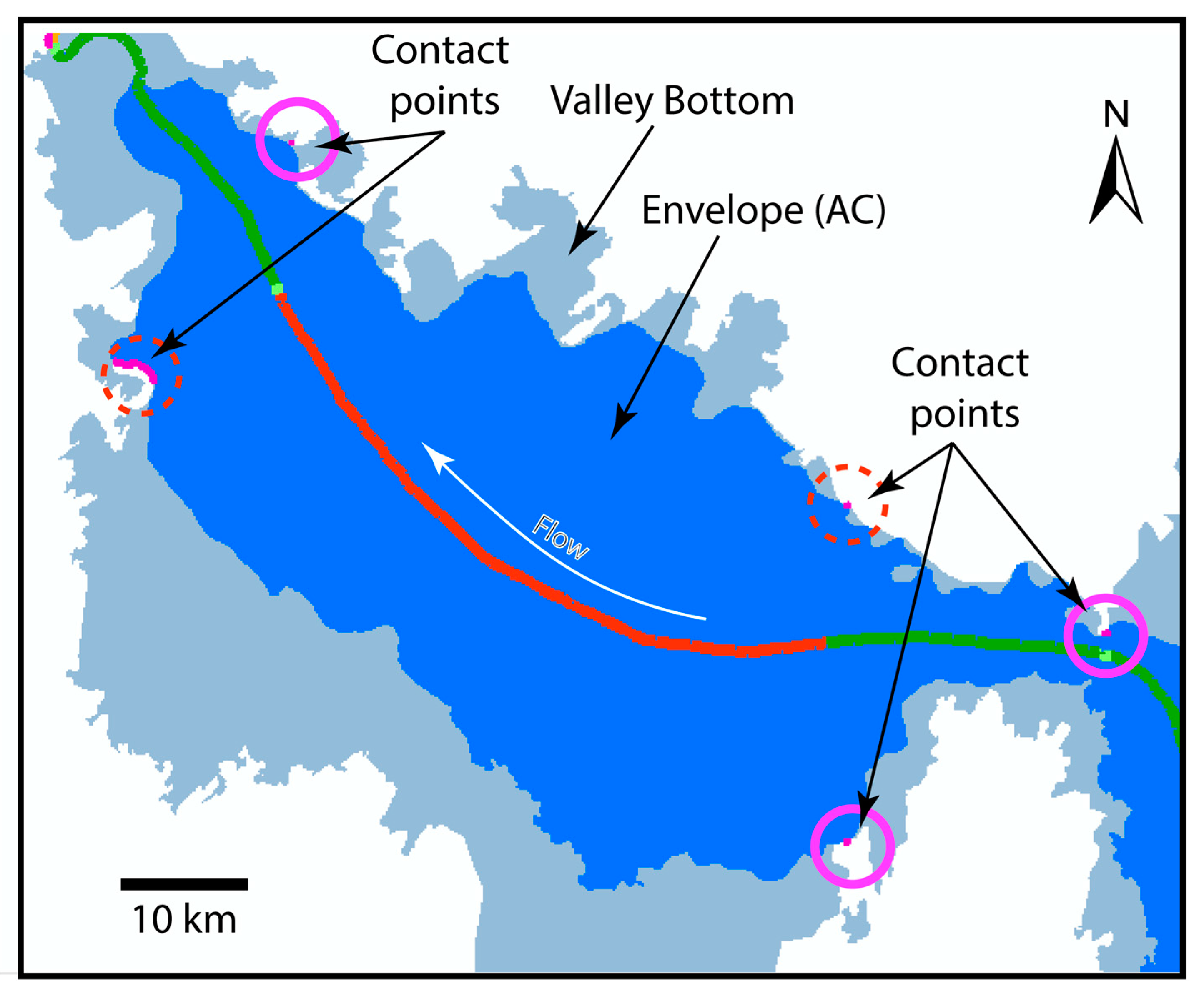
O’Brien’s algorithm implements a peculiar way to obtain a holistic synthesis, starting from reductionist analytical information associated with short river segments. We found that this may lead to inconsistencies (as shown in Figure 4) or even mistakes (possibly due to our inappropriate use?), when the river is anastomosed with a very wide envelope of the active channels (“AC envelope” in what follows) (see Figure 5). Moreover, the assumption concerning the cause of confinement is evidently arbitrary and, furthermore, cannot include the frequent case of confinement by infrastructure (e.g., railways, roads, levees). Finally, it does not compute an explicit statistical indicator: the classification is obtained only by assigning a color scale.
In general, the algorithm produces a somehow hysterical sequence of different confinement categories (in this case: mostly laterally unconfined with two shorter segments partly confined) and is not able to capture a more holistic character (indeed, we would classify the whole stretch as partly confined). Notice in Figure 4 that while the output of the algorithm is reported along the reference axis adopted (colored polyline axis: dark green: unconfined; light green: partly confined planform controlled; orange: partly confined valley margin controlled; red: confined (not detected in this figure along the axis)), to assess confinement one has to look at the blue polygon representing the envelope of active channels (which is wide or very wide where the river is anabranching or anastomosed), and identify sectors where it touches either margin of the VB polygon (grey area). Only the red contacts count because even though other lines seem in contact, visually, from a geographical point of view (GIS) they are not: sometimes, indeed, the difference amounts to a few meters only, but it is still larger than the tolerance adopted in the buffer used by the algorithm.
The algorithm we developed in GeoMagda overcomes such difficulties. As already stated, it assumes that the reaches over which the confinement statistical indicator is to be computed are already defined. This is the basic difference with O’Brien’s algorithm.
Other differences, which constitute additional advantages, are as follows:
it is accessible to any user of ArcGIS (or QGIS) and Excel;
it computes an explicit statistical confinement indicator;
it determines the cause of confinement, if provided with the polyline of the VB margins separated in categories: valley margin, planform, or infrastructure.
Our algorithm undoubtedly suffers from some limitations: It is designed for isolated rivers (not a river network); the current version is based on the number of discretized short-segments with a contact (the “numerosity”), not on the actual contacts length; and it is not automated, which means that it requires a rather large number of manual (but not expert based) steps that, as a whole, can be quite cumbersome. However, with a sufficiently fine discretization, there is no actual gain in considering the length of the short segments rather than their numerosity; and automatizing such a procedure is perfectly possible.
In Appendix B we provide details of the algorithm, so that it can be replicated step by step; Figure 6 provides a general idea of the first part, related only to confinement.

3.2. A Logical Heuristic “Reductionist→ Holistic Algorithm” for Mono-Dimensional Variables

We address here the need to obtain a holistic synthesis from reductionist information. The expression “Reductionist → Holistic” refers to the attempt to translate information related to an attribute at the local level (e.g., the width of the active channel or the presence/absence of islands within a short segment of the river) into information that synthesizes, in general, multiple attributes and with a view that spans well beyond the single short-segment. In the particular mono-dimensional applications presented below, the reductionist information is the local presence/absence value (binary case) or else the specific value within a finite set of possibilities (categorical case), while the holistic synthesis is a judgment obtained by looking at a sequence of such reductionist values along the river, identifying homogenous stretches. To this aim, we developed a logical heuristic algorithm, both for the binary and thee categorical cases, whose results are nicely consistent with expert judgment output. We adopt the term “logical heuristic” to stress the fact that the algorithm is based on explicit reasoning (logics), but with some steps that not necessarily lead to an optimum, although still achieving the purpose (at least in our application).

3.2.1. Reductionist → Holistic Algorithms: The Literature Status

For the mono-dimensional problem (only one attribute), a statistical approach seems to be the best option. Parker et al. [20] provide an interesting literature synthesis of statistical algorithms borrowed from geological analysis [21], recalling Davis’ classification scheme [22] in (i) “local boundary hunting” and (ii) “global zonation”. The former searches for the boundary between two distinct levels of the considered character; e.g., Webster’s algorithm [23] and its variants identify the location of “breaks” by sliding a moving window until the difference of variance before and after its midpoint is maximized, while variance is kept at a minimum within each one of the two halves. it’s the performance depends on the width of the moving window, a variable which is selected somewhat arbitrarily. The second approach, “global zonation”, looks at the whole data set at a glance, trying to identify those subsets of points that are internally most uniform. For instance, Bohling et al.’s [24] cluster algorithm identifies first that location characterized by the minimum change of any possible couple of adjacent points within the dataset. These two adjacent zones with the smallest difference are then combined into one combined zone, which is treated as a single object, characterized by the mean value of the points within the zone, and considered in the next iteration. The process continues, with more and more zones being joined based on their similarity to each other. This method begins with zero within-zone variance, but each iteration results in an increase, until the proportion of total variance explained by the zonation falls below a specified threshold. Other “global zonation” methods, however, like Gill, [25] and Hawkins and Merriam, [26], are better suited for the identification of river reach boundaries because they statistically minimize within reach variation and maximize between reach differences, and are less influenced by local inconsistencies in the data sequence. Gill’s method explicitly seeks to identify the zonation that minimizes the variance within each zone (reach) and maximizes the difference between the zones (reaches). Hubert [27] introduced an algorithm which works in a similar manner; although it is possibly the best performing one for this task, its outputs are not exempt from questioning (Figure 7). Similar conclusions have been found by other researchers (e.g., Martinez-Fernandez et al. [28]).
Furthermore, it must be recognized that all of these approaches have been designed thinking of quantitative, continuous (scalar) variables; when binary variables are concerned instead, they conceptually and practically fail. This is particularly true for Hubert’s test, which is considered the key tool to define separate reaches within the Fluvial Corridor ToolBox [29]. This is one of the reasons why we explored a different approach by developing logical heuristic algorithms.
For evaluating the performance of algorithms, Parker et al. [20] assume that the higher the proportion of variability R is explained by the reach boundaries, for a given number of reaches, the stronger the performance, and hence the zonation algorithm is best suited to defining functional river reaches. Operationally (what follows has been slightly reformulated and corrected from Parker et al. [20]) R is equal to Equation (1):
R = σ2zone/(σ2zone + σ2stretch)
where σ2zone is a measure of the variance of the reach means about the grand mean μ of the whole sequence, defined as follows Equation (2):
σ2zone = [∑j=1…mj − μ)2]/(m − 1)
where σ2stretch, j, m and μj are defined as follows Equation (3):
σ2stretch = ∑j=1…m[ ∑i=1…nj (xij − μj)2]/[N − m]
where x ij is the i th point within zone j , μj is the mean of the j th zone, n j is the number of points in the j th zone, N = (∑j=1…nj) is the total number of points considered amongst all zones, and m is the number of zones.
The closer the performance index R gets to 1, the better the output is, because this means that the intra-cluster variances countless (i.e., they are smaller because cluster data are more similar to cluster mean), while the difference amongst clusters (expressed as the variance of the clusters means) increases and becomes the dominant component of the differentiation. Thus, one has clusters internally more homogeneous and more diverse amongst them.
Although very reasonable, this criterion is not suitable for our case. Indeed, as is apparent from what follows, our algorithm tries to “give life” to all cases of “presence” as soon as they form a sequence sufficiently long (actually longer than LM), without leaving “holes” longer than LM, being this a significant length parameter to be set. So, the performance must be assessed on this basis. At the moment, we just considered ourselves satisfied with the visual appreciation.

3.2.2. Reductionist→ Holistic Algorithm: The Binary Case

In this case, the variable of interest is assessed at a number of points along the river in terms of presence/absence (usually corresponding to a relatively dense discretization as presented in Figure A1Appendix A). Hence, the algorithm presented here operates on a binary variable (0,1) that maps the original variable over a fine discretization of the river axis into segments. We assume that the character of the river is assessed over a stretch of meaningful length, in no case shorter than a stretch with a “minimum significant length” LS. The philosophy interpreted by the proposed algorithm is hence in a few words: “identify those stretches, not shorter than LS, to which a predominant value can be assigned”.
The algorithm operates as follows:
choose a significant minimum river length LS, basically according to the usual criterion of LS = 10 ÷ 20 W, where W is the width of the envelope of active channels. This minimum length corresponds to a number K of segments (K = Ls/d, with d length of a discretization segment) and their associated values of the considered variable;
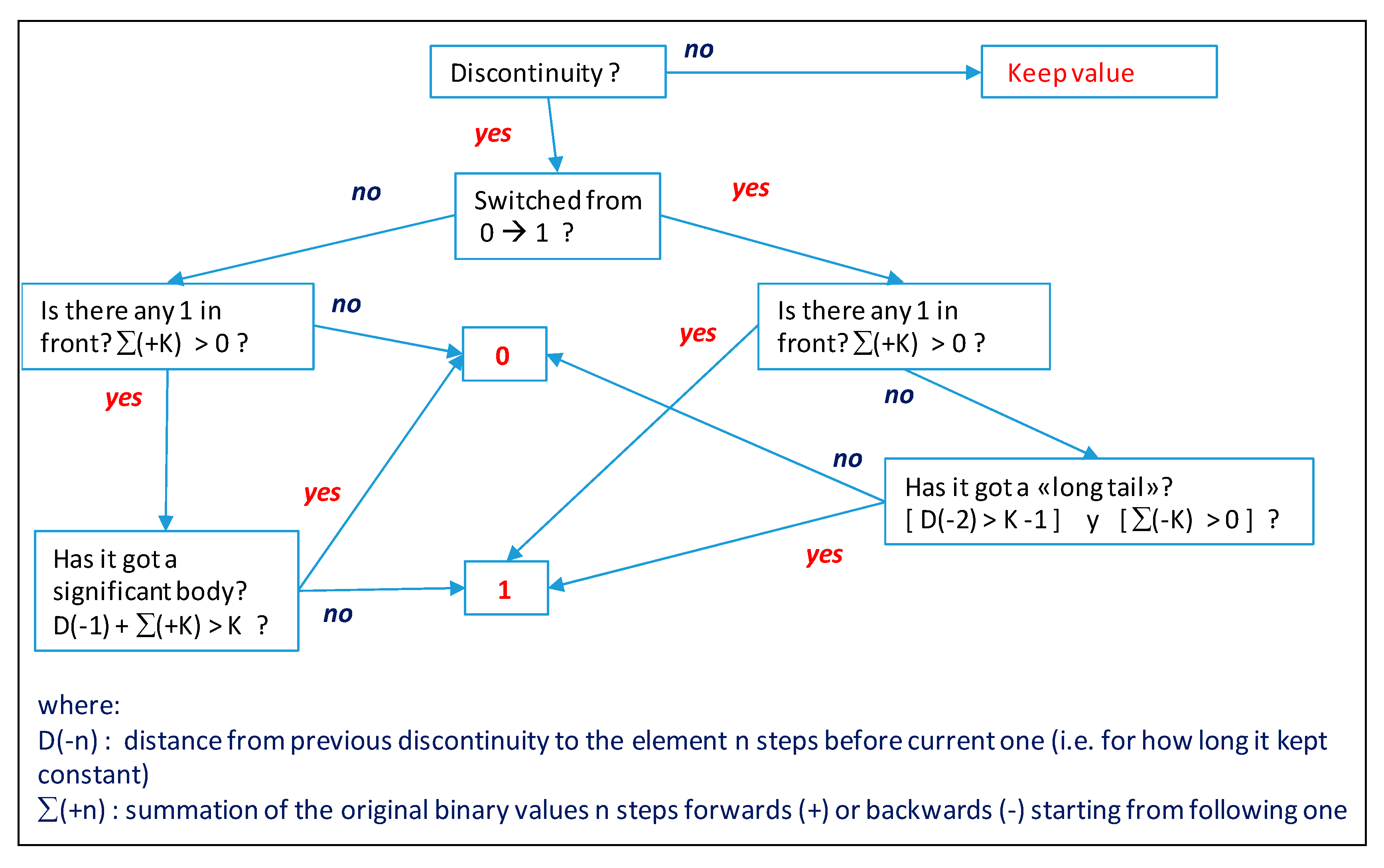
identify the discontinuity points, i.e., locations where the binary indicator (measuring the relevant attribute) changes from 0 to 1 or vice versa, and determine the distance D(-1) from the previous discontinuity (the notation D(-n) denotes the number of points separating previous discontinuity from the segment located n steps before current one);
if the current point is not a discontinuity, then just keep the original value of the variable; if it is a discontinuity, instead, “look forward and backwards” to ascertain whether the discontinuity is due just to a local effect (“absence’, i.e., a “hole”, or “presence”) or it is the beginning of a new reach within the significant horizon, and assign the new value accordingly (see Figure 8).
All of this results in a sequence of value for the new binary variable (0,1) “presence” called “Holistic 1”.
Now, run the following procedure for the newly calculated binary variable Holistic 1:
identify new discontinuities for this new variable;
to each one, apply a forward moving averaging (on the K horizon) operator and, if the result is less than the threshold α, come back to a 0 value (absence), otherwise set it to 1;
in this way, obtain a sequence of values for the new binary variable “presence” called “Holistic 2”;
in this series, filter out all reaches characterized by absence, but shorter than the minimum significant length LS;
obtain thus a sequence of values for the new binary variable “presence” called “Holistic 3”;
in this series, filter out all reaches characterized instead by presence, but shorter than the minimum significant length.
Result is the final sequence of values for the binary variable called “Holistic ok”.
This algorithm can be run for a “minimum significant length” LS varying along the river, according to the fluctuating (generally increasing) width of the active channel envelope.
We are aware that this is just a first version that can certainly be improved (some steps are perhaps unnecessary); however, as shown in the next section, it performs quite nicely, at least in our case study.

3.2.3. Binary Case: Application to Magdalena River’s Islands

“Presence of islands” is an example of a binary attribute where a manipulation of the originally assessed values (1: presence, 0: absence of an island in each discretization segment) may be of interest if one wants to come up with an identification of reaches “with islands” as distinguished from those “without”.
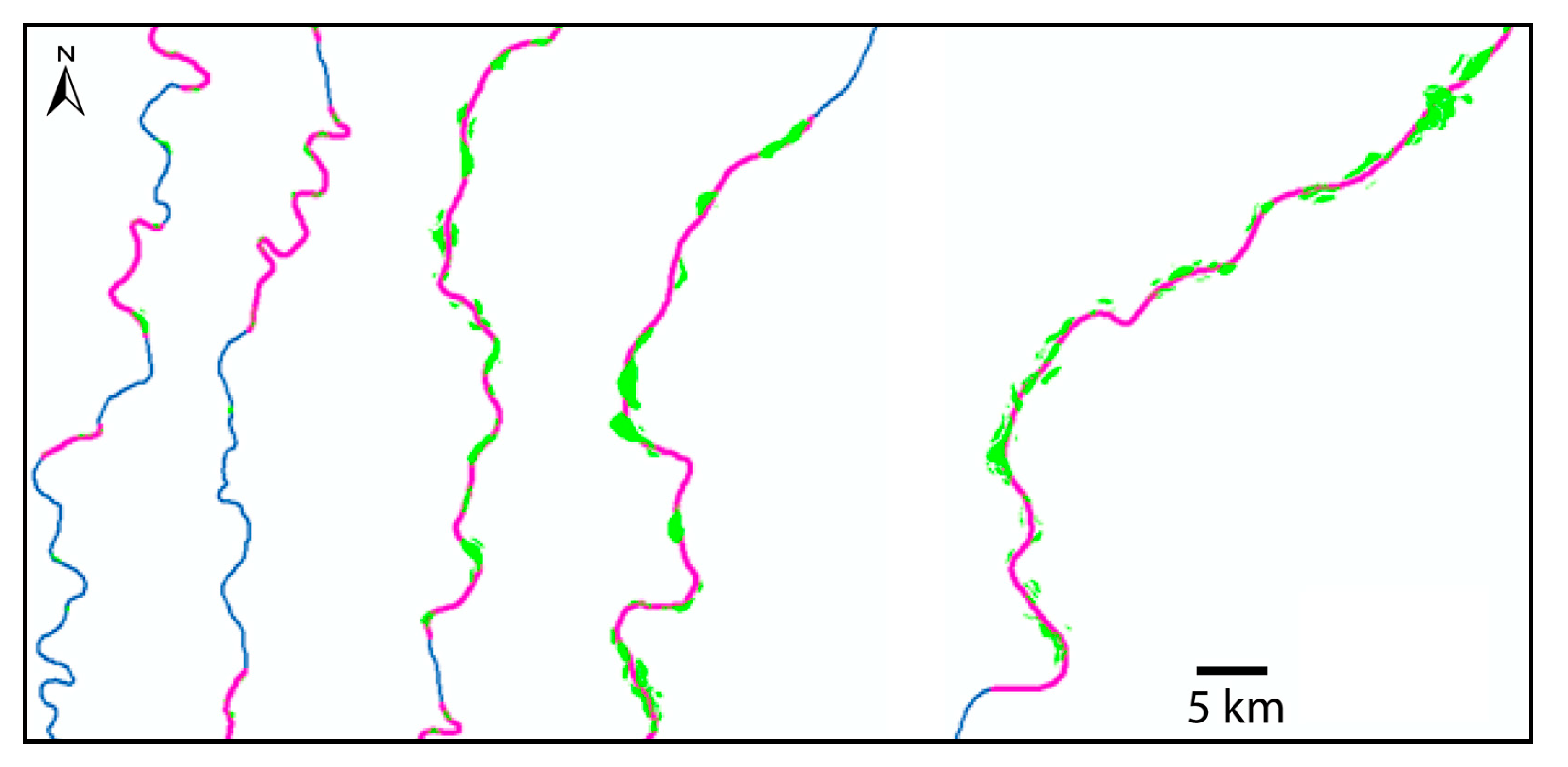
From Figure 9, it can be observed that no reaches shorter than the established significant length LS are left; but also that sometimes (particularly, in the first reach at the bottom of the first stretch at the left) isolated (tiny) islands appear in a stretch labelled as “no islands”; this is an expected result that is consistent with the way the algorithm is set up.

3.2.4. Reductionist→ Holistic Algorithm: The Categorical Case

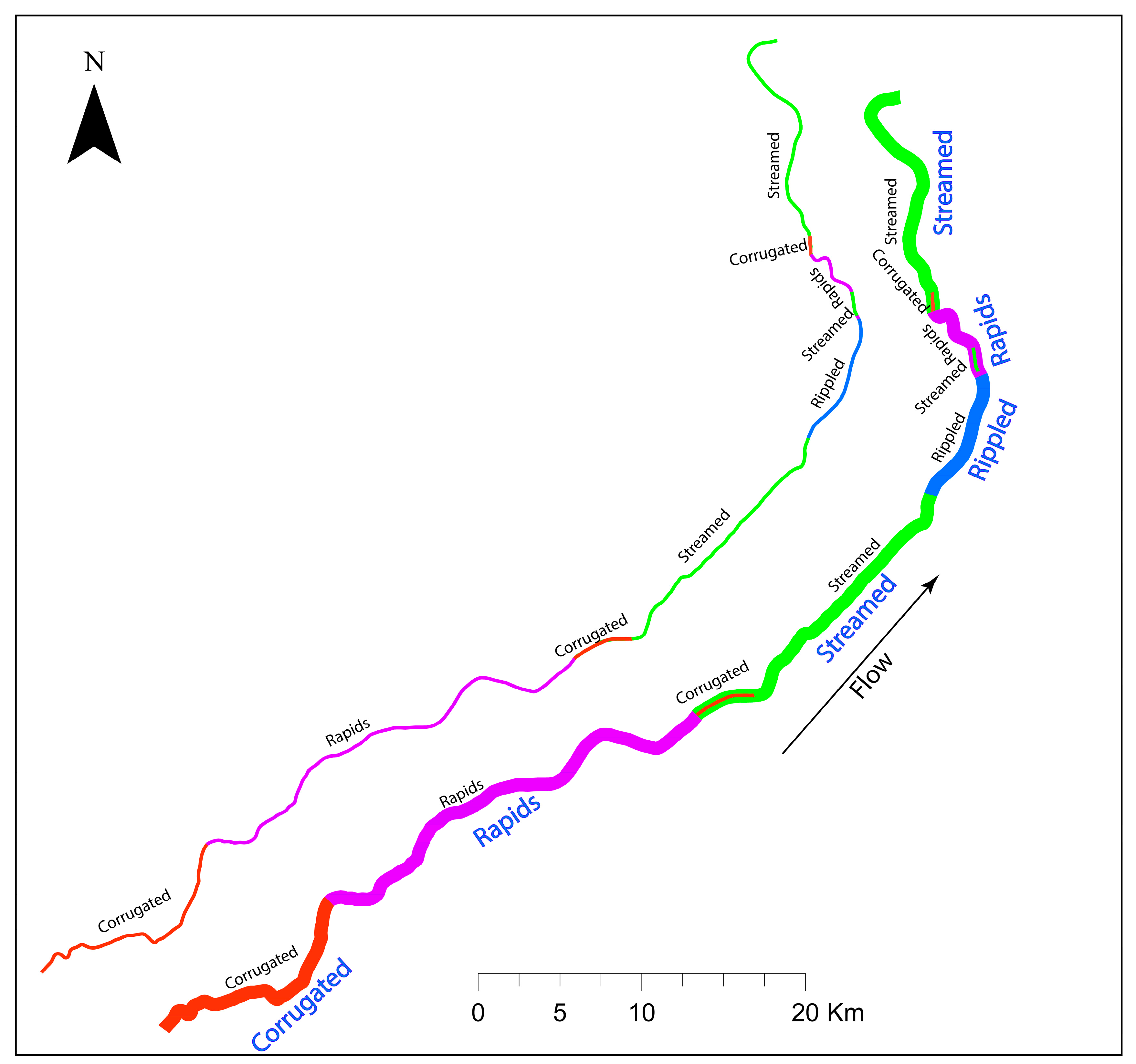
A categorical variable assumes discrete values defined over a non-ordinal scale (i.e., it is not possible to rank them in any order). As an example, for the Cauca River (main tributary of the Magdalena) we created a variable denoted “current,” related to the type of surface flow (as recognizable from Google Earth imagery; this is a proxy for “character of the bed,” a variable that cannot be assessed directly for turbid rivers like these, where the bed is in general not visible). The variable “current” has seven possible categories (and corresponding discrete values on a non-ordinal scale):
0: rapids; 1: corrugated (long riffles that do not end in a pool); 2: pool and riffle; 3: streamed (stretch with visible lines of current and local turbulence, but softer than in previous cases); 4: rippled (softer than streamed); 5: plane surface (probably corresponding to planar bed: runs or glides); 10: not detectable (bad quality of images).
The philosophy for the holistic algorithm in this case is very simple: “do not leave windows shorter than LS and assign to each stretch the prevailing value in it”. It can be noted that this algorithm is structurally “rougher” than in the binary case because there is not a clear criterion to choose which category to keep when a stretch is too short and hence we adopted a very simple and practical criterion that, although working acceptably well, could be well substituted by others.
Hence, the proposed algorithm works as follows:
Cycle I:
Identify discontinuities (where switches from one category to any other occur).
Where no discontinuity is present, the algorithm keeps the previously calculated value (as a result of this holistic algorithm; at the first step it assumes the original value).
Where a discontinuity occurs:
-
“K steps forward prevailing”: the algorithm identifies that category which occurs with the highest frequency in the K steps downstream.
-
"Residual frontal window": analogous, but along just K–D(-1) steps forward (this is a forward moving horizon which progressively narrows down within a fixed window starting from the previous discontinuity; it is modified when a switch occurs to the next discontinuity). Its purpose is to consider what the prevailing value was previous to the current point.
-
When the prevailing value in the residual forward window coincides with that previous to the last discontinuity → current segment is just a “local hole” and as such the algorithm keeps the previous holistic value.
-
When the value is "not detectable" (one of the 7 possible categories), the algorithm just keeps it.
-
If not, the algorithm takes the same value of the prevailing category within the K steps forward.
Cycle II: removing residual segments shorter than K steps.
Here the following (arbitrary) criterion is adopted: “just make them uniform with the previous adjacent category”. Hence, the algorithm goes like this:
-
It identifies the discontinuities in the result from Cycle I.
Where no discontinuity is present, it keeps the previous value (the new one, produced by the algorithm; where a discontinuity occurs instead:
-
If the full distance from the previous discontinuity is smaller than K, the algorithm assigns the same value occurring before the discontinuity.
-
If not, it keeps the current value.
Again, the fitness criterion here is purely visual (Figure 10).

4. Conclusions

We can honestly say that the proposed systematic procedure and set of computer-aided tools (the ToolBox, some of whose tools we presented herein) do provide a significant benefit. An objective and systematic identification of reaches (addressed in Nardini et al., [18]), a reliable (although perhaps somehow cumbersome) confinement procedure, the reductionist-holistic tools, and the automatic, GIS based, grouping tool (not described in detail here: see Table A1 of Appendix A) provide all together a substantial support.
We are aware that the procedure reported in Table A1 and the specific algorithms and tools we developed (e.g., the confinement tool) still require a significant manual intervention and sometimes not straightforward exchanges between GIS and Excel; in other words, the proposed procedures are automatable, but not yet fully automated. All this, however, lies just at the operational level; what really matters is that the expert judgment is actually needed only in specific, well identifiable tasks: the definition of criteria like the Procedural Tree; the fine revision of the VB identification; the overall interpretation of the river behavior; and progressively less, the mapping of geomorphic units (but this is very likely to be soon performed by automatic procedures as discussed, for instance, in Piégay et al. [1]).
The conceptual clarifications and operational procedures, tools, and hints provided within the ToolBox and associated Manual can significantly support many practitioners—particularly in the Spanish-speaking world—and can help disseminate the adoption of the River Styles Framework, as well as the use of the Fluvial Corridor ToolBox.

Author Contributions

Conceptualization: A.N. and S.Y.; Methodology: A.N. and S.Y.; Software: S.Y.; Validation: A.N., S.Y., and M.D.B.; Formal analysis: A.N. and S.Y.; Investigation: A.N., S.Y.; Data curation: A.N. and S.Y.; Writing—original draft preparation: A.N.; Writing—review and editing: A.N., S.Y., M.D.B.; Project administration: A.N.; Funding acquisition: A.N. All authors have read and agreed to the published version of the manuscript.

Funding

This research received external funding thanks to The Nature Conservancy through the “GeoMagda” Project, contract No. TNC-CREACUA NASCA 00162/2018.

Acknowledgments

We thank Gary Brierley and Kirstie Fryirs for the stimulating exchanges of ideas in the development of the GeoMagda project. We warmly thank the team of Hervé Piégay (Université de Lyon, FR) for helping us exploring and understanding their Fluvial Corridor ToolBox and then discussing weaknesses and potential improvements, particularly through exchanges with Christophe Rousson, Antonio Aurelie, and Michel Kristell. We are also grateful for the postdoctoral support for the second author during this research with funds from the PAUSE programme of the Collège de France (Contrat d’Engagement n° 04055876) and the collaboration of the Research Institute for Development in France (IRD). Finally, we warmly thank Claudio Meier (University of Memphis, USA) for his invaluable support in reviewing English language; nevertheless, the responsibility for residual imperfections is fully in our hands.

Conflicts of Interest

The authors declare no conflict of interest.

Appendix A

Table A1. Steps operationally needed to carry out a full River Styles (Stage I, Steps 1 and 2) analysis and corresponding tools/procedures proposed for doing so. Bold italic type items are those we developed “ex-novo” and which are fully described in the ToolBox Manual; two of these—“Confinement tool” and “Reductionist → Holistic algorithm”—have been described in the text above (Section 3.1). Notice that in our application to the Magdalena River Basin, described in [16,17], we adopted a set of official digital ArcGIS shapefiles that allowed us to skip some of the steps related to the delineation of geomorphic elements and units (but not all), but at the same time raised some issues mainly due to resolution and lack of synchronicity with the available Digital Elevation Model (DEM) from the Shuttle Radar Topography Mission (SRTM) 30 m filled.
ObjectAlgorithmTool/ProcedureObservations
MethodologyProcedural Tree and definition of attributesChoose structure suited for the case at hand conserving a river basin (or even better, a regional) perspectiveExpert judgementThis is where expert judgment is mainly involved
InstrumentalDEM clipped to the area of interestSelect and extract zone of interestManual: ArcGIS TOOL CLIP (Data Management) according to a rectangle mask or EXTRACT by MASK, given a polygon (i.e., the river basin)
InstrumentalLandforms (terraces, fans…)Expert judgement (from aerial photographs, field surveys, …)ManualWith a high-resolution DEM some degree of automation is possible (e.g., TerEX by Stout and Belmont, [8])
InstrumentalGIS reference pointsLocate points along the axis of VB (see below) at constant distanceStandard GIS procedures (creating points along a line)These are very useful to orient the analyst while quickly switching from GIS to Google Earth
InstrumentalGeographical reference pointsExpert judgement (towns, known sites, appropriate density, closeness to river, manageable number, etc.)Manual construction of a point GIS Shapefile (SHP)Sites useful to guide descriptions and to show in schematics and maps
InstrumentalBase segmentation pointsLocation where there is an evident change of VB width, catchment area (tributary); break in slope; discontinuities (dams)Manual standard GIS procedures. Possibly use FCT: Disaggregation; Metrics (width, etc.), Statistics (Hubert’s test) and Metrics (Discontinuities)Can be used as a preliminary indication to define reaches (e.g., VB width well identifies macro reaches)
InstrumentalType of VB marginIdentification of infrastructure and landform mappingManual by standard GIS proceduresFirst the effective valley bottom must be defined (see below)
InstrumentalContact points river-valley marginIdentify key points where the envelope of active riverbed (see below) touches the margin of the effective VB. Geological, planform, and anthropogenic contacts should be consideredManual, expert judgment procedure on GIS supported by DEM info + standard construction of a GIS point SHP (semi-automatic GIS algorithms are an alternative)Useful to assess degree of "constraint" and sediment sources, particularly in laterally unconfined (but constrained) reaches. Active channels’ envelope needs to be determined first (see below)
InstrumentalContact segments between active riverbed and VB marginsCreate a thin buffer around the envelope of the active riverbed; then intersect with the effective VB (see below)Manual standard ArcGIS procedures (buffer, intersection)It is a basic information for the confinement attribute. Active channels’ envelope must be determined first (see below)
InstrumentalSediment sourcesIdentify where there is: a contact point with landslides, fans or terraces; or meanders with external VB elevation higher than internal (so that the erosion-sedimentation balance is positive); or a tributary inputManual (expert based) or semi-automated GIS proceduresThe expert judgment can be synthesized in a logical tree that can then be implemented (even in an Excel spreadsheet) to carry out this task
InstrumentalConstrictionsIdentify where:-VB is narrow: (V-W local)/W < α-the reach is single thread and not excessively "spread"; i.e.,: [ W–w]/w < β -The envelope significantly reduces with respect to the upstream average: [W–W ]/W > γ. Where: CA: active river bed (set of active channels); V: VB width (and V: moving average); W: width of envelope (W: moving average); w: width of active river bed; and: α,β,γ: parameters.Excel spreadsheet (GeoMagdaToolBoxManual: "Esqueleto_magda")A constriction is not a contact point, but a short reach where the VB narrows down significantly, at the local scale, as compared with upstream and downstream. Constrictions are important because they can induce changes in hydraulic and sediment behavior and, consequently, in morphology
InstrumentalSegmented VBSpatial discretization of the VB according to regular reaches along its centerline with a relatively fine step (e.g., 500 m for the Magdalena) and sequenced (i.e., spatially ordered)FCT: Disaggregation; SequencingThis is a very important step that supports several subsequent steps. The key output is the “Rank_DGO” field of the obtained table.
Geomorphic
elements
Active channel “just water”Satellite images interpretation. For Magdalena: use of official SHP IGAC 100 mil “Drenaje doble” already available; separation of branches not completely connected and tributaries-ArcGIS procedure: calculation of indices like MNDWI (the Modified Normalized Difference Water Index) [30,31], selection of pixels over threshold, transformation to polygon, cleaning-Manual, expert judgment in ArcGISIt is important to use images referring to high waters, but actual overbank flooding should be avoided. Automatic algorithms suffer from presence of clouds
Geomorphic
elements
Active riverbed (CA) (collection of active channels completely connected, including bars, but not islands)Add mid channel and bank attached bars to the "active channel just water” polygon. NOTICE: The procedure presented here refers to the specific information available for the Magdalena, where an official SHP IGAC 1:100,000 was available for bars ("bancos de arena") but did not discriminate amongst main river and tributaries. It must be noted that this SHP presents some inconsistencies; it was probably built based on different, asynchronous images, possibly by different operators.ArcGIS procedure: -draft (still without bars) envelope of active channels (see next step); -buffer of this envelope of a max width of lateral bar; -CLIP the original bars SHP (IGAC 2017 100 mil «bancos de arena») with this envelope; -manual check to eliminate bars not belonging to the river of interest; -MERGE with the active river bed; DISSOLVECare must be put in not including bars belonging to tributaries; there is a degree of ambiguity. A more direct procedure consists of identifying bars directly from satellite images as bare surfaces, based for instance on the SWIR (Short-wavelength infrared) band (band 7 in OLI (The Operational Land Imager), TIRS (Thermal Infrared) and TM (Thematic Mapper) Landsat missions), as shown in Monegaglia et al. [32]
Geomorphic
elements
Envelope of active riverbed (collection of connected active channels)Transform the polygon into a polyline SHP and eliminate all lines different from the external boundaryArcGIS procedure:-Tool «Feature to Line»; -manually eliminate internal small polygons; -retransform into a polygon with «Feature to Polygon»; -finally, possibly use «Smooth Polygon» (Cartography)This is not a "convex hull", but the polygon ideally obtained by merging the polygons of all active channels fully connected
Geomorphic
elements
IslandsEliminate the active riverbed (including bars) from the envelope of active riverbedArcGIS: ERASEAlternatively, interpretation of satellite images with appropriate indices (e.g., NDWI, Carlson and Ripley, [33]) can be carried out. However, the procedure suggested here ensures consistency
Geomorphic
elements
Bank-attached barsEliminate the envelope of active riverbed "just water" (which, by construction, includes islands and mid channel bars) from the envelope of active riverbed (CA)ArcGIS: ERASEAlternative methods exist; for instance, the GUT tool within the River Scape Community ([34,35,36]), but they just work with high resolution imagery and altimetry. UAV surveys can provide viable alternative at moderate scales of analysis (e.g., Casado et al. [12] or for a review: Carrivick and Smith, [3])
Geomorphic
elements
Mid-channel barsEliminate the active riverbed "just water" and island sand bank attached bars from the envelope of active riverbedArcGIS: ERASE tripleSame observation as above
Geomorphic
elements
Axis of active riverbedCenterline of the envelope of active riverbed-FCT (Tool 1.3 Centerline), or ToolBox Manual (Módulo Básico 2): tool based on ArcGIS/ArcScan which provides a more smoothed output-PyRIS proposed by Monegaglia et al. [32]: the tool identifies the axis of the main channel even in anabranching rivers, defined either as the widest or the longestFor RS application, a centerline is sufficient and perhaps preferable because in anabranching rivers, selecting a particular branch may be less representative.
Geomorphic
elements
Natural valley bottom (VB)Identify the portion of flat land adjacent to the river and not higher than a given threshold. Build to this aim various DEM of Differences (DoD) with various thresholds and check consistency with land-use, envelope of contemporary flooded areas (e.g., from the Dartmouth Flood Observatory database: https://www.dartmouth.edu/~floods/, specifically the derived product “Annual flooded areas”), geomorphic map, field evidencesFCT: Spatial Components; 1.2 valley bottom. See however various details explained in the ToolBox Manual, "Modulo VB". Other tools exist like for instance VBET [37], but with no particular advantagesEven with a perfect DEM, a manual correction is needed because of several reasons, e.g., the DEM may have captured the elevation of water, not of riverbed and hence the DoD is at least ambiguous.
Geomorphic
elements
Effective VBEliminate from Natural VB portions separated by works that may interrupt channel migration or flooding (e.g., roads, railways, rip-rap protections)Manual procedure in ArcGIS. In the ToolBox Manual, "Modulo Básico 8", a systematic procedure is proposed-
Geomorphic
elements
Axis of effective VBCenterline of the envelope of effective valley bottomTotally analogous to "Axis of active riverbed"-
RS
Attributes
Sediments (bed material texture)Construction of a point SHP in each sampling or survey station and transformation to a line SHP (based on the Axis of Active Channel) assuming some interpolation criterion-Physically sample or adopt some imagery interpretation tool (e.g., [38,39]) -Interpolation: assume that the sampled texture holds until next station, possibly with expert-judgment adjustments; or: use an algorithm to translate reductionist information into a holistic synthesis like the "HOLISTICO binario" Excel Tool-
RS
Attributes
PlanformIdentify reaches with a recognizable combined pattern of number of channels, distance, width, sinuosity and number, size and position of islands and bars.-Expert-based identification based on satellite imagery (e.g., Google Earth) and available polygons of active riverbed. Supported by ToolBox Manual: “Modulo FCT 3.4 Morphometry” for sinuosity and “Modulo sinuosidad nueva”; “Modulo MonoMulti canales” for single/multi thread (see this paper). -Alternatively, use the automated Excel tool presented in Nardini et al. [16]a-Single thread: rectilineous, sinuous, meandering, irregular, tortuous. b-Transitional: wandering; alternate bars; “swallowing” (i.e., still single thread and mainly straight or sinuous, with local significant widening, including one or more islands. c- Multi thread: braided; island braided; anabranching avulsive; anastomosed; combinations.
RS
Attributes
Streamflow characterIdentify reaches with a recognizable pattern of current threads, turbulence, areas of still water. (for rivers where the riverbed is visible at low flow, a similar attribute would be “bed morphology”)-Expert judgement or - Other Tools like GUT (see above) -interpolate with reductionist-holistic “HOLISTIC categorical” Excel ToolGoogle Earth imagery brings in ambiguities because of varying quality, date and time of the images.
RS
Attributes
Presence of natural leveesIdentification of elements from aerial or satellite imagery (e.g., Google Earth) and DEM; holistic synthesis of the reductionist information into meaningful stretches; translation reporting into a polyline along active riverbed axis with binary attribute (presence/absence)Expert judgement + info from existing reports → construction of a polygon SHP Then: GIS intersection of such SHP with the segmented effective VB (from FCT); translation into a binary attribute (presence/absence) along the discretized VB axis (GIS procedure); finally, translation into a polyline (presence/absence) along the VB axis with the “ HOLISTICO binario” Excel Tool (see above); possibly, transposition into a polyline along the axis of the active river bed with the Excel Tool “De_VB_a_CA”For the first step of identification, alternatively, GUT Tool or similar can possibly be used. The transposition from the discretized VB axis into the axis of the active river bed is not trivial because, owing to their different location in the floodplain, a different number of segments from discretization may occur. All this is explained in detail in the ToolBox Manual (Modulo Basico 5 and 6)
RS
A.
Presence of wetlandsanalogousanalogousanalogous
RS
A.
Presence of paleo channelsanalogousanalogousanalogous
RS
A.
Presence of oxbowsanalogousanalogousanalogous
RS
A.
Presence of ridge & swale topographyanalogousanalogousanalogous
RS
A.
Presence of bank-attached barsanalogousanalogousanalogous
RS
A.
Presence of mid-channel barsanalogousanalogousanalogous
RS
A.
Presence of islandsanalogousanalogousanalogous
RS
Attributes
ConfinementIdentification of contact lengths (see above) and computation of a statistic indicator over the reaches of the selected segmentationManual ArcGIS procedure as detailed in the ToolBox Manual Modulo 3 bis (this paper)Confinement is a statistical indicator defined over an ordinal scale, assessed for each reach, with values: “confined”, “partly confined”, “laterally unconfined”
RS
Attributes
Cause of confinementFor each confined or partly confined reach, identifies which is the prevailing cause amongst: “valley”, “planform”, “works” (anthropogenic)Manual ArcGIS procedure as detailed in the ToolBox Manual Modulo 3 bis (this paper)In each reach, several causes may intervene; the prevailing one in terms of lengths involved (adding right and left bank) is considered
RS
A.
ConstraintsExpert judgement based on the contact points already identifiedManual on ArcGIS
SynthesisReachesAccording to Nardini et al. [16], we identify independent segments according to non-extensive attributes: Planform; Bed material texture; Streamflow character, finding the “least common, spatial denominator”(see Nardini et al. [18])The reaches are the basis for the Geo database and to support visualization of attributes
SynthesisGeoDB (polyline GIS SHP segmented according to reaches)Assign to each reach a value for each one of the relevant attributes. For those directly involved in the definition of reaches, just select the appropriate value associated with the original segmentation; for the remaining ones (belonging to the Procedural Tree), compute a statistic, ordinal indicator (e.g., for binary cases like local presence/absence of a geomorphic unit: 1: “absent”, 2: “occasional”, 3: “frequent”, 4: “prevailing”, 5: "complete”)For: Cause of confinement: see Excel Tool “CONFINA” in the ToolBox Manual. For binary attributes it is the % of reach length where the attributes presents a “YES” value: see Excel Tool ESTADIS_TramosAccording to our Procedural Tree, the attributes requiring a statistical computation are:-confinement-cause of confinement-geomorphic units within the VB (levees, oxbow, ridge and swale, paleoCH, wetlands)-geomorphic units within the channels (bank attached and mid channel bars, islands; streamflow character)
SynthesisSkeleton (finely discretized, polyline GIS SHP)Discretize the VB axis in short segments (e.g., 500 m for the 1400 km long VB axis of the Magdalena River); compute a metric for each attribute relevant to generate a meaningful synoptic scheme (distances, elevation, contributing catchment area; active river bed width, VB width, valley slope); build an area- bankfull flowrate relationship (Qb = Qb(A)) and determine total and specific streampowerFCT: 3. Metrics (in each segment, the Tool computes several values, e.g., every 50 m within a 500 m segment, and offers sub-statistics)Skeleton is better constructed along the axis of the valley bottom in order to represent planform sinuosity. In the Magdalena exercise, owing to the low DEM resolution, FCT did not work to determine the contributing catchment area; a manual ArcGIS procedure was adopted instead and then data were processed within the Excel “Tool ESQUELETO”
SynthesisSynoptic scheme (profile and plan view)Build a sketch in Excel (both profile and plan view) by using the Skeleton information and reference points SHP.A suitable filter (e.g., moving average plus not decreasing condition) must always be applied to the original elevation data from DEM, particularly when referring to the VB axis because this is an idealized line that often crosses planforms or hills (an example is offered in the Excel Tool ESQUELETO)There must be one for each river considered in the basin (in our preliminary exercise Magdalena and Cauca rivers). It is appropriate to include in the main river sketch (Magdalena) the long profile for all tributaries
SynthesisMacro scale mapMap the relevant information (possibly available from existing cartography): landscape units, faults involving the rivers; active channels; reference points; effective VB; macro scale confinement; planform (or at least single-multi thread segments); cause of confinement (VB margins); constrictionsStandard ArcGIS mapping proceduresAll relevant rivers are presented in a same map. This is split into a minimum number of whole basin maps because merging too much information is confusing; so, the clearest, but most synthetic combination must be sought
ClassificationRiver StylesIdentify the reaches with the same combination of values of main attributes, according to the Procedural Tree adopted (e.g., planform, bed material texture, confinement, cause of confinement); do the same with all attributes.Python/ArcGIS Tool (ToolBox Manual): see ToolBox Manual and Nardini et al. [16,17]Owing to ArcGIS limitations, currently it supports only 7 attributes at a time; therefore, the process might need to be split in more than just two cycles. Actually, we needed three for the Magdalena:I cycle: main ones → Label Main II cycle: Label Main + 5 geomorphic units within the VB → Label II. III cycle: Label_II + 4 geomorphic units within the channel

Appendix B

Appendix B.1. B—Determining Confinement

Our procedure is as follows:
(i)
Identify local confined segments (contact between the AC envelope and VB margins, analogously to O’Brien et al. [6]):
-
create a small buffer of the AC envelope (delta = 10 ÷ 20 m for the Magdalena; this is a parameter to be “calibrated” according to the river at hand);
-
apply “ERASE tool” of the output polygon with the VB polygon → the output is a SHP of small «contact» polygons (it is possible to transform them into lines, but it is not necessary);
-
apply “BUFFER tool” of such contact polygons with the same delta (set ArcGIS options as: Side type = FULL and Dissolve = NONE);
-
add an integer field (CONF);
-
separate the right from the left part by ERASE using two masks defined from the AC axis: use Right Mask for left part and vice versa.
(ii)
Determine a local confinement indicator within the Skeleton, by using the spatial correspondence between contact segments and discretization “slices” obtained for instance with the Fluvial Corridor ToolBox (see Table A1) to this aim:
-
apply “Spatial Joint tool” of the contact segments (polygons), first left and then right, with the effective, segmented VB (and sequenced, i.e., with a spatial order, output of a FCT tool which automatically includes the “Rank_DGO” field) as target;
-
assign (with Select by attribute and field calculator) 1 if there is no empty intersection (i.e., there is local confinement) or 0, if vice versa;
-
thus, obtain the segmented VB with the binary 0-1 field for confinement (two polygon SHP for left and right sides). What is useful in this SHP table is the “CONF” columns;
-
extract the SHP table in an Excel spreadsheet; Sort on the basis of the Rank_DGO field;
-
apply “PASTE tool” in it these two columns (one at a time) and the Rank_DGO column (the Excel Tool CONFINA can be used for this purpose).
(iii)
obtain the final statistical indicator over the selected reaches (polyline SHP “Reaches” with final segmentation chosen to assess confinement); notice that such reaches typically have varying lengths. The statistical indicator can simply be the ratio of the total number of either bank confined slices falling within a reach, over the total number of slices within that reach. To this aim:
-
insert a field “ID_Reach” into the table of the .shp Reaches, with-increasing value;
-
apply “Spatial Join tool” of the segmented SHP VB with this .shp Reaches (using VB as Target to obtain a complete correspondence of elements);
-
export the table and correct manually because, once ordered base on the Rank_DGO field, “holes” may appear (i.e., “0” values in the middle of a sequence of a given value corresponding to a long segment: this is caused by the fact that the axis of the AC may not intersect all the elements of the VB, as shown in Figure A1) in the ID_Tramos column: these must be filled. In this way, this instrumental Excel will now contain two fields (say “CONF_sx” and “CONF_dx”) with the correspondence of elements between Skeleton (discretization “slices”) and reaches;
-
in the same Excel it is now possible to compute the statistical indicator: The final product is a polyline SHP Reaches including a discrete attribute with (typically) the three categories “confined, partly confined, laterally unconfined”.
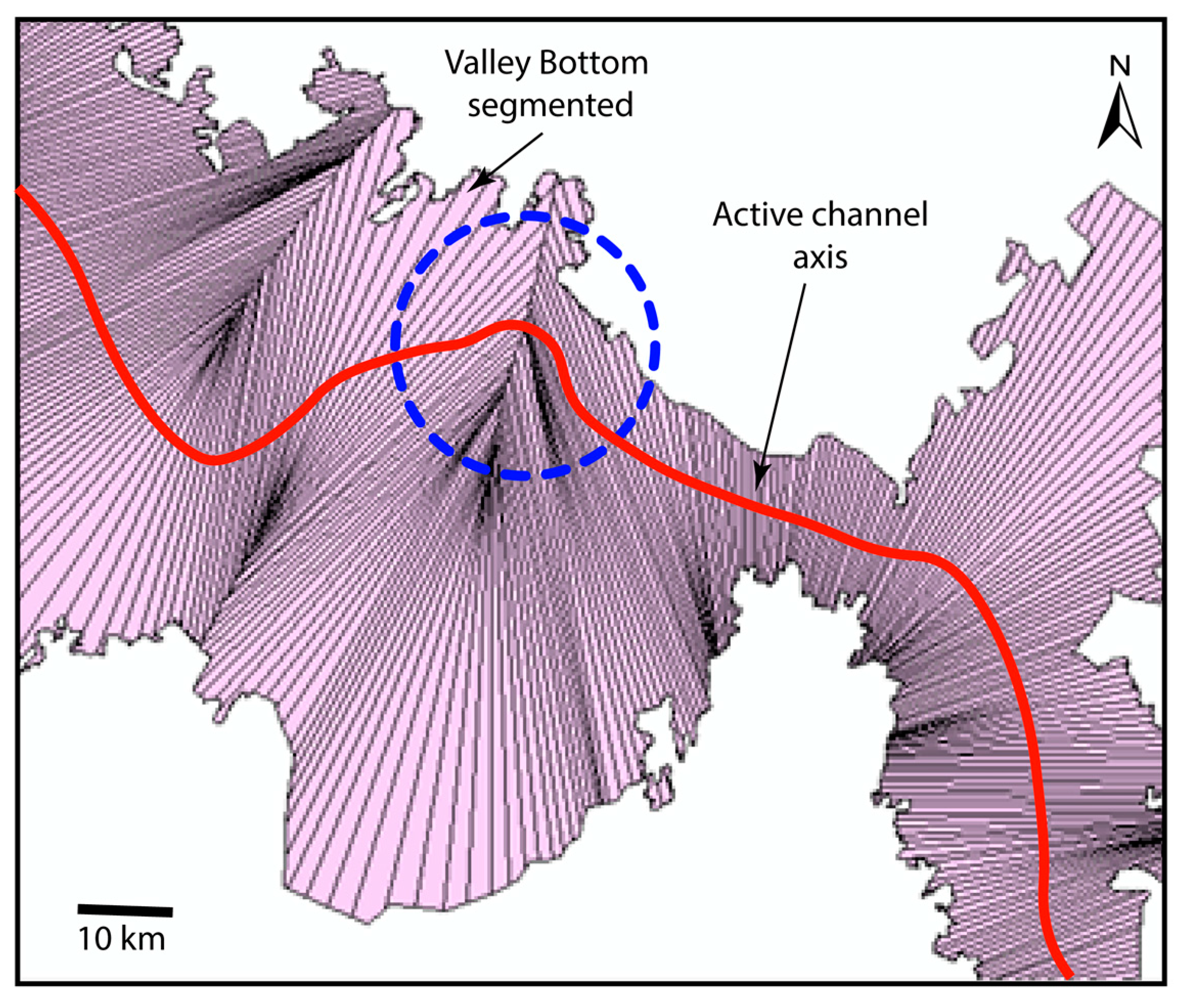
Figure A1. Example (blue, dotted circle) of a situation where the segmentation of the VB may create an inconsistency with a line SHP (e.g., the AC axis, red line): the line does not touch all segments because some of them do not cross the whole VB polygon. Therefore, the intersection line-segmented VB will not contain the same number of elements; but the identifiers of those remaining will be correct.
Geosciences 10 00231 g0a1

Appendix B.2. B—Determining the Cause of Confinement

This part includes two stages (1) and (2) which are described in this section:
(1)
Build a VB margin polyline SHP with an attribute "Type of margin" (valley, planform, and infrastructure). To this aim:
(i)
Take the effective VB (already possibly cut by infrastructure and as such with margins in contact with them) and build a polyline SHP with two separate lines (right and left): the ArcGIS Tool “Feature to Line” can be adopted, then cutting the contour line at the beginning and end; add a field "Type of margin".
(ii)
Determine locations with binding infrastructure (by using polyline SHP of roads, railways, dykes, longitudinal defenses, gabions, batteries of groynes, etc.), that is, where the natural VB has been cut by some infrastructure thus originating an effective VB; to this aim, one possibility is as follows:
-
buffer of VB with +10 and another buffer with−10 (for the Magdalena);
-
take the spatial “difference” (ERASE) obtaining a kind of strip;
-
with this strip get the intersection with line works (CLIP) → obtain a polyline SHP of the interfering works;
-
make a BUFFER of such SHP;
-
apply the Analysis Tools/Overlay/IDENTITY Tool between the polyline SHP VB margin and this SHP of interfering works after applying a BUFFER tool to it;
-
apply the tool MULTIPART TO SINGLE PART to the result;
-
where there actually is an intersection (Select by Attribute), assign Type = “work” (with the Field calculator). Typically, the output is very fragmented, but this is not a problem as afterwards it is only used to compute a statistical indicator.
(iii)
Determine where the margin is “planform” (a polyline SHP of the planforms must be available; a possibility is to build it by identifying surfaces at differential height from a sufficiently precise DEM); to this aim:
-
apply IDENTITY between the SHP VB margins and the SHP planforms;
-
then, in editing mode, by Select by attribute select all those items that are not “works” AND with non-empty intersection and assign Type = “planform”. To the remaining ones assign type = “valley”;
-
finally, add a length field and compute it (by Geometry option) and clean the SHP by eliminating all useless fields other than margin (Left, Right) and the type → obtain the polyline SHP VB margins with attribute Cause of confinement.
(2)
Produce the information needed to compute the statistical indicator to be associated with each "Reach" of the segmentation adopted for Confinement (as described above). Namely, this means producing a polyline SHP segmented and sequenced exactly as the VB (same elements), including:
-
the identifiers (ID) of the VB slice
-
the ID_Reach
-
the Type of margin (left and right, separated).
To this aim:
(0)
apply the BUFFER tool to the polyline SHP of Type of VB margin;
(i)
split it into a right and a left SHP utilizing the masks already obtained (above);
(ii)
with each one, apply a SPATIAL JOIN with the segmented VB as target;
(iii)
extract their Excel tables; ensure the completeness of the corresponding series of VB IDs (by filling where needed the “holes”, analogously to what has been shown above);
(iv)
use the left and right columns ordered according to the Rank_DGO field to compute the statistical indicator that just selects the type of confinement with maximum number of contact slices within each Reach. To this aim, the Excel Tool CONFINA can be used (described in the GeoMagda ToolBox).
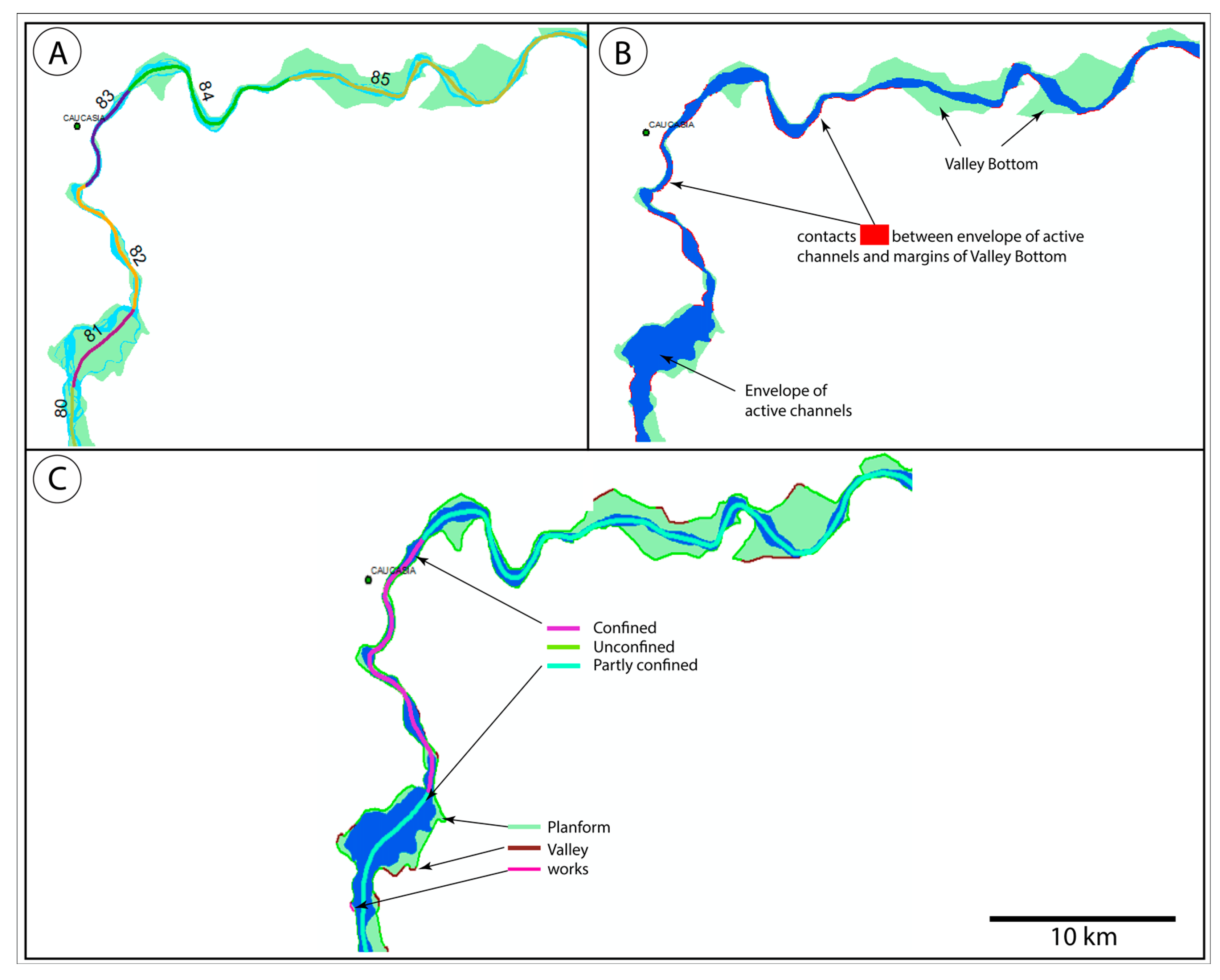
Figure A2 presents the outputs obtained for the Cauca River (Colombia) with the above described algorithm.
Figure A2. Example of output for a stretch of the Cauca River from the proposed confinement algorithm: A) active channel (narrow, light blue polygon), VB (light green polygon) and reaches (identified by colors of the axis segments); B) identification of contacts (small red segments or dots); C) confinement categorical indicator and types of margins of the VB. Notice that several contiguous reaches have the same confinement classification (e.g., 80, 81, bottom left in A, are partly confined; 82, 83 confined), but different type of Cause of confinement (because of different type of VB margin) and hence are displayed in a different color.
Geosciences 10 00231 g0a2

References

  1. Piégay, H.; Arnaud, F.; Belletti, B.; Bertrand, M.; Bizzi, S.; Carbonneau, P.; Dufour, S.; Liébault, F.; Ruiz-Villanueva, V.; Slater, L. Remotely sensed rivers in the Anthropocene: State of the art and prospects. J. Earth Surf. Process. Landf. 2020, 45, 157–188. [Google Scholar] [CrossRef]
  2. Brierley, G.; Fryirs, K. Geomorphology and River Management: Applications of the River Styles Framework; Wiley-Blackwell: Malden, MA, USA, 2005. [Google Scholar] [CrossRef]
  3. Carrivick, J.L.; Smith, M.W. Fluvial and aquatic applications of Structure from Motion photogrammetry and unmanned aerial vehicle/drone technology. J. Wiley Interdiscip. Rev. Water 2018, 6, e1328. [Google Scholar] [CrossRef] [Green Version]
  4. Fryirs, K.A.; Wheaton, J.M.; Bizzi, S.; Williams, R.; Brierley, G.J. To plug-in or not to plug-in? Geomorphic analysis of rivers using the River Styles Framework in an era of big data acquisition and automation. J. Wiley Interdiscip. Rev. Water 2019, 6, e1372. [Google Scholar] [CrossRef]
  5. Fryirs, K.A.; Brierley, G.J. Assessing the geomorphic recovery potential of rivers: Forecasting future trajectories of adjustment for use in management. J. Wiley Interdiscip. Rev. Water 2016, 3, 727–748. [Google Scholar] [CrossRef]
  6. O’Brien, G.R.; Wheaton, J.M.; Fryirs, K.; Macfarlane, W.W.; Brierley, G.; Whitehead, K.; Gilbert, J.; Volk, C. Mapping valley bottom confinement at the network scale. J. Earth Surf. Process. Landf. 2019, 44, 1828–1845. [Google Scholar] [CrossRef] [Green Version]
  7. Clubb, F.J.; Mudd, S.M.; Milodowski, D.T.; Valters, D.A.; Slater, L.J.; Hurst, M.D.; Limaye, A.B. Geomorphometric delineation of floodplains and terraces from objectively defined topographic thresholds. J. Earth Surf. Dyn. 2017, 5, 369–385. [Google Scholar] [CrossRef] [Green Version]
  8. Stout, J.C.; Belmont, P. TerEx ToolBox for semi-automated selection of fluvial terrace and floodplain features from LiDAR. Earth Surf. Process. Landf. 2014, 39, 569–580. [Google Scholar] [CrossRef]
  9. Wheaton, J.M.; Brasington, J.; Darby, S.E.; Sear, D.A. Accounting for uncertainty in DEMs from repeat topographic surveys: Improved sediment budgets. J. Earth Surf. Process. Landf. J. Br. Geomorphol. Res. Group 2010, 35, 136–156. [Google Scholar] [CrossRef]
  10. Bizzi, S.; Blamauer, B.; Braca, G.; Bussettini, M.; Camenen, B.; Comiti, F.; Demarchi, L.; Garcia De Jalon, D.; Gonzalez Del Tanago, M.; Grabowski, R. Thematic Annexes of the Multi-Scale Hierarchical Framework. Deliverable 2.1, Part 2 of REFORM (Restoring Rivers for Effective Catchment Management), a Collaborative Project (Large-Scale Integrating Project) Funded by the European Commission within the 7th Framework Programme under Grant Agreement 282656; European Commission: Brussels, Belgium, 2014. [Google Scholar]
  11. Bizzi, S.; Demarchi, L.; Grabowski, R.; Weissteiner, C.; Van de Bund, W. The use of remote sensing to characterise hydromorphological properties of European rivers. J. Aquat. Sci. 2016, 78, 57–70. [Google Scholar] [CrossRef] [Green Version]
  12. Casado, M.; Gonzalez, R.; Kriechbaumer, T.; Veal, A. Automated identification of river hydromorphological features using UAV high resolution aerial imagery. J. Sens. 2015, 15, 27969–27989. [Google Scholar] [CrossRef] [Green Version]
  13. Dalla Mura, M.; Prasad, S.; Pacifici, F.; Gamba, P.; Chanussot, J.; Benediktsson, J.A. Challenges and opportunities of multimodality and data fusion in remote sensing. J. Proc. IEEE 2015, 103, 1585–1601. [Google Scholar] [CrossRef] [Green Version]
  14. Demarchi, L.; Bizzi, S.; Piégay, H. Hierarchical object-based mapping of riverscape units and in-stream mesohabitats using LiDAR and VHR imagery. J. Remote Sens. 2016, 8, 97. [Google Scholar] [CrossRef] [Green Version]
  15. Demarchi, L.; Bizzi, S.; Piégay, H. Regional hydromorphological characterization with continuous and automated remote sensing analysis based on VHR imagery and low-resolution LiDAR data. J. Earth Surf. Process. Landf. 2017, 42, 531–551. [Google Scholar] [CrossRef]
  16. Nardini, A.; Yépez, S.; Rogeliz, C. Caracterización geomorfológica river styles en la Cuenca del rio Magdalena: Caso estudio Magdalena y caja de herramientas para la aplicación automatizada a la cuenca. GeoMagda ToolBox; The Nature Conservancy: Bogotá, Colombia, 2019; Available online: https://www.researchgate.net/publication/338585128_Manual_GeoMAGDA (accessed on 3 March 2020).
  17. Nardini, A.; Yepez, S.; Zuniga, L.; Gualtieri, C.; Bejarano, M.D. A Computer Aided Approach for River Styles—Inspired Characterization of Large Basins: The Magdalena River (Colombia). Water 2020, 12, 1147. [Google Scholar] [CrossRef] [Green Version]
  18. Nardini, A.; Yepez, S.; Mazzorana, B.; Ulloa, H.; Bejarano, M.D.; Laraque, A. Geomorphic river characterization: A systematic, automated approach for river segmentation with case studies on the Magdalena River (Colombia) and on the Baker River (Chile). Water 2020. submitted. [Google Scholar]
  19. Nagel, D.E.; Buffington, J.M.; Sharon, P.L.; Seth, W.; Goode, J.R. A landscape scale valley confinement algorithm: Delineating unconfined valley bottoms for geomorphic, aquatic, and riparian applications USDA For. Serv. Gen. Tech. Rep. RMRS-GTR 2014, 42. [Google Scholar] [CrossRef] [Green Version]
  20. Parker, C.; Clifford, N.J.; Thorne, C.R. Automatic delineation of functional river reach boundaries for river research and applications. J. River Res. Appl. 2012, 28, 1708–1725. [Google Scholar] [CrossRef] [Green Version]
  21. Harmar, O.P.; Clifford, N.J. Planform dynamics of the lower Mississippi River. J. Earth Surf. Process. Landf. 2006, 31, 825–843. [Google Scholar] [CrossRef]
  22. Davis, J. Statistics and Data Analysis in Geology; John Wiley and Sons: New York, NY, USA, 2002; p. 656. [Google Scholar]
  23. Webster, R. Automatic soil-boundary location from transect data. J. Int. Assoc. Math. Geol. 1973, 5, 27–37. [Google Scholar] [CrossRef]
  24. Bohling, G.; Doveton, J.; Guy, B.; Watney, L.; Bhattacharya, S. PFEFFER 2.0 Manual; Kansas Geological Survey: Lawrence, KS, USA, 1998. [Google Scholar]
  25. Gill, D. Application of a statistical zonation method to reservoir evaluation and digitized-log analysis. J. AAPG Bull. 1970, 54, 719–729. [Google Scholar]
  26. Hawkins, D.M.; Merriam, D. Optimal zonation of digitized sequential data. J. Math. Geol. 1973, 5, 389–395. [Google Scholar] [CrossRef]
  27. Hubert, P. The segmentation procedure as a tool for discrete modeling of hydrometeorological regimes. J. Stoch. Environ. Res. Risk Assess. 2000, 14, 297–304. [Google Scholar] [CrossRef]
  28. Martínez-Fernández, V.; Solana-Gutiérrez, J.; del Tánago, M.G.; de Jalón, D.G. Automatic procedures for river reach delineation: Univariate and multivariate approaches in a fluvial context. J. Geomorphol. 2016, 253, 38–47. [Google Scholar] [CrossRef]
  29. Roux, C.; Alber, A.; Bertrand, M.; Vaudor, L.; Piégay, H. “Fluvial Corridor”: A new ArcGIS ToolBox package for multiscale riverscape exploration. J. Geomorphol. 2015, 242, 29–37. [Google Scholar] [CrossRef]
  30. Feyisa, G.L.; Meilby, H.; Fensholt, R.; Proud, S.R. Automated Water Extraction Index: A new technique for surface water mapping using Landsat imagery. J. Remote Sens. Environ. 2014, 140, 23–35. [Google Scholar] [CrossRef]
  31. Xu, H. Modification of normalized difference water index (NDWI) to enhance open water features in remotely sensed imagery. J. Int. J. Remote Sens. 2006, 27, 3025–3033. [Google Scholar] [CrossRef]
  32. Monegaglia, F.; Zolezzi, G.; Güneralp, I.; Henshaw, A.J.; Tubino, M. Software Automated extraction of meandering river morphodynamics from multitemporal remotely sensed data. J. Environ. Model. 2018, 105, 171–186. [Google Scholar] [CrossRef]
  33. Carlson, T.; Ripley, D. On the relation between NDVI, fractional vegetation cover, and leaf area index. J. Remote Sens. Environ. 1997, 62, 241–252. [Google Scholar] [CrossRef]
  34. Bangen, S.; Kramer, N.; Wheaton, J.; Bouwes, N. The GUTs of the Geomorphic Unit Tool (GUT): What is under the hood. In Proceedings of the AGU Fall Meeting, New Orleans, LA, USA, 11–15 December 2017. [Google Scholar]
  35. Bangen, S.G.; Kramer, N.; Wheaton, J.M.; Bouwes, N. Mapping instream geomorphic units from high resolution topography. 2020; In preparation. [Google Scholar]
  36. Kramer, N.; Bangen, S.; Wheaton, J.M.; Bouwes, N.; Wall, E.; Saunders, C.; Bennett, S.; Fortney, S. Geomorphic Unit Tool (GUT): Applications of Fluvial Mapping. In Proceedings of the AGU Fall Meeting Abstracts, New Orleans, LA, USA, 11–15 December 2017. [Google Scholar]
  37. Gilbert, J.T.; Macfarlane, W.W.; Wheaton, J.M. The Valley Bottom Extraction Tool (V-BET): A GIS tool for delineating valley bottoms across entire drainage networks. J. Comput. Geosci. 2016, 97, 1–14. [Google Scholar] [CrossRef]
  38. Carbonneau, P.; Fonstad, M.A.; Marcus, W.A.; Dugdale, S.J. Making riverscapes real. J. Geomorphol. 2012, 137, 74–86. [Google Scholar] [CrossRef]
  39. Carbonneau, P.E.; Lane, S.N.; Bergeron, N.E. Catchment-scale mapping of surface grain size in gravel bed rivers using airborne digital imagery. J. Water Resour. Res. 2004, 40. [Google Scholar] [CrossRef] [Green Version]
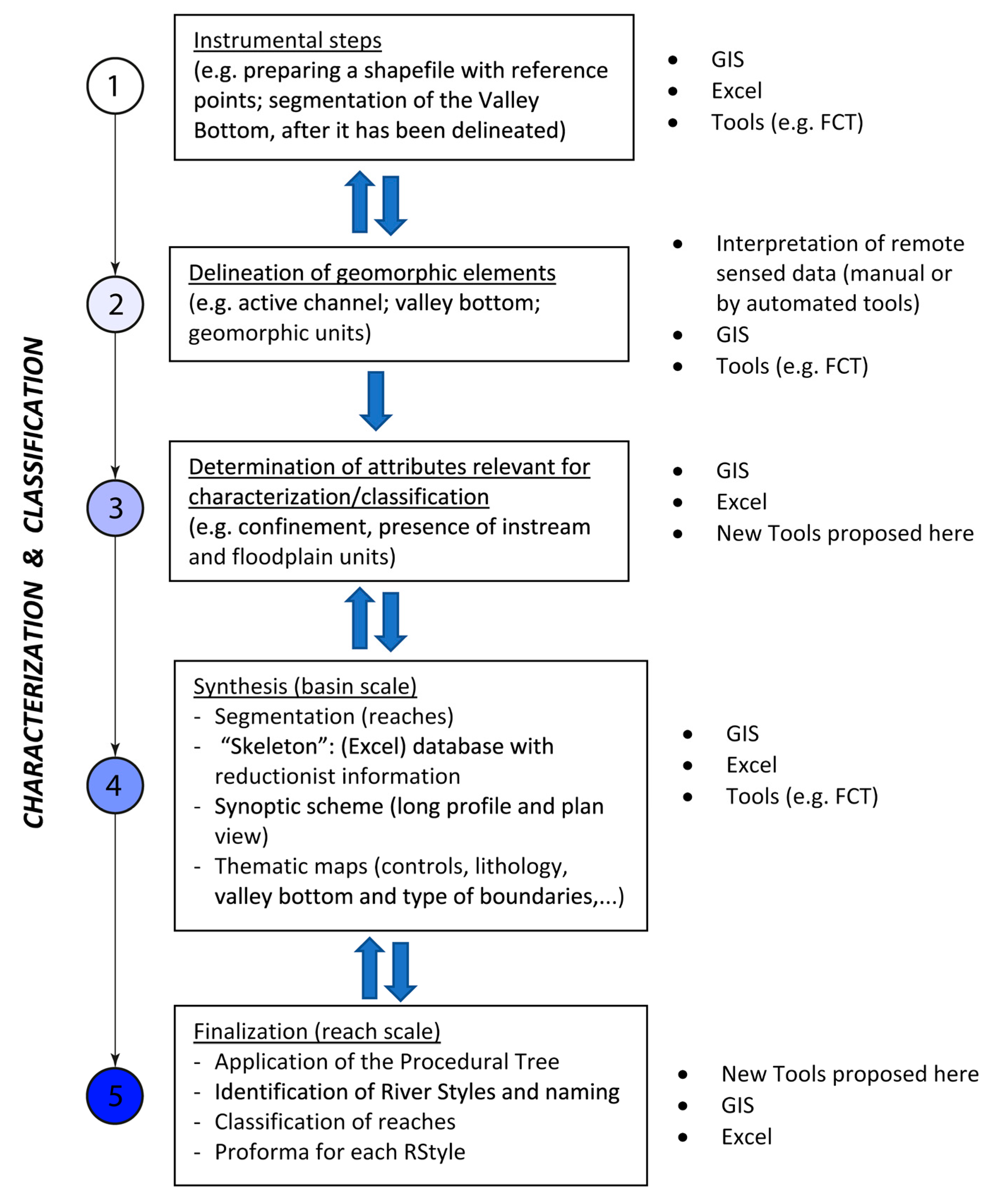
Figure 1. Scheme of the whole procedure proposed for the River Styles inspired characterization and classification of rivers within a basin (the Procedural Tree is the structured set of attributes adopted in the River Styles Framework (RS) analysis to characterize river reaches; Proforma is the standardized document adopted again in the RS analysis to described in a more detailed fashion each particular River Style found. Additional details are provided in Appendix A). FCT = Fluvial Corridor ToolBox.
Geosciences 10 00231 g001
Figure 2. Confinement strongly depends on the segmentation (scale of analysis) adopted. Left: zoom of a segment fully confined (red lines at the border indicate contacts), at its specific scale; middle: a stretch of a river classified as partly confined at the given scale of analysis (the contacts between valley bottom (VB) margins and the active channel are marked with red, solid line); right: zoom of another segment fully unconfined, at its specific scale.
Geosciences 10 00231 g002
Figure 3. Map of the Magdalena basin highlighting some of the tectonic controls and the macro-scale confinement.
Geosciences 10 00231 g003
Figure 4. Examples of unsatisfactory output we obtained with O’Brien et al. [6] algorithm (Upper Magdalena River, approx. 10 km downstream of Neiva town: 867490.92; 823535.51 MAGNA Colombia Bogota, see Figure 3 to locate the town in the basin).
Geosciences 10 00231 g004
Figure 5. Inconsistent output from O’Brien et al. [6] algorithm, which reports a long river stretch as “confined” (red axis; green represents “laterally unconfined”, instead) while in reality it only presents two small contact points (small red dotted circles), one at its beginning (top, right, corresponding to the beginning of the red stretch) and one at its end (bottom, left). The blue area is the envelope of the Active Channels (AC) that in this particular case cover a very wide area as the river is anastomosed. The pale blue-grey area is the valley bottom.
Geosciences 10 00231 g005
Figure 6. Steps for calculating Confinement: (1) Intersection between the valley bottom (VB) and a buffer of the Active Channel (AC) to determine contacts; (2) Determination of the correspondence between contacts and segmented VB (by applying mainly the FCT and obtaining the Discretized Geographical Objects (DGO)); (3) Determine the spatial correspondence between VB segments and contacts using the GIS tool “Spatial join”; (4) Determine the Confinement Type by applying a statistical rule using an Excel spreadsheet on the attribute table extracted from the segmented VB shapefile.
Geosciences 10 00231 g006
Figure 7. Example of segmentation of a continuous, quantitative attribute (the VB width of a stretch of the Magdalena River) via Hubert’s statistical test (as implemented in the FCT): the output (stretches of different colors) is questionable as, for instance, the segment delimited by the two red lines (amongst many others) would certainly be classified by expert judgment as narrower than the one above it (notice that there is no criterion linked to the length, as Hubert’s test determined both short and long segments).
Geosciences 10 00231 g007
Figure 8. The logical heuristic, binary attribute, Holistic algorithm implemented for the Magdalena River. Notice that this figure—for simplicity- does not represent the full algorithm, but the essence of its logics and as such the intermediate variables Holistic 1, 2, 3 are not identifiable, nor is the role of the threshold α.
Geosciences 10 00231 g008
Figure 9. Results of the application of the binary, logical heuristic Holistic algorithm developed for the Magdalena River, as applied to the attribute “presence of islands”. Several consecutive stretches are presented (the river flows from bottom-left to top-right). The small green polygons are the original islands (then transformed into a 0÷1 indicator in the discretized VB, not shown here); the resulting linear attributes along the active bed axis (centerline) takes the pink color, with a thicker line, when the holistic indicator of presence of islands is “yes” and the blue, thinner line, when it is “no”. The significant length adopted is Ls = 5 km, shown at the bottom right, as the prevailing river width is W = 500 m (therefore, K = Ls/d = 10, as we assumed d = W).
Geosciences 10 00231 g009
Figure 10. Example of application of the “Holistic categorical” algorithm for the Cauca river (Magdalena basin), for the attribute “current” (which can assume the values: “rapids, corrugated, pool & riffle, streamed, rippled, plane surface, not detectable”). Left: original values (with black labels) along a stretch, which can sometimes refer to very short segments. Right: the same stretch after the application of the proposed categorical holistic algorithm in thick line over the original thin line (same one of the left figure): it can be seen that the number of segments has now been significantly reduced (blue labels with larger font), no segment is shorter than the adopted significant length LS, and the reaches that were “engulfed” are those that were originally the shortest.
Geosciences 10 00231 g010