1. Introduction
With the advent of new satellite constellations for positioning, the navigation scenario has observed a strengthening of satellite availability. New systems like Galileo and BEIDOU2 have been put beside the well-consolidated systems like the U.S.A.’s GPS and Russia’s GLONASS. With such a quick improvement of the Global Navigation Satellite Systems (GNSS) scenario, the future receivers must be able to take advantage of these potentials. From this perspective, SDRs (Software-Defined Receivers) can be very useful tools for both researchers and surveyors. In fact, despite the fact that commercial receivers can assure great performance, they are a black box, limiting the possibilities of upgrades. On the other hand, SDRs are capable of extreme customization, allowing users to access, visualize, and maybe modify signal acquisition, tracking, and processing strategies. SDR refers to an ensemble of hardware and software technologies and design choices that allows re-configurable radio communication architectures. The main idea behind this concept is the replacement of the dedicated hardware components by means of software modules.
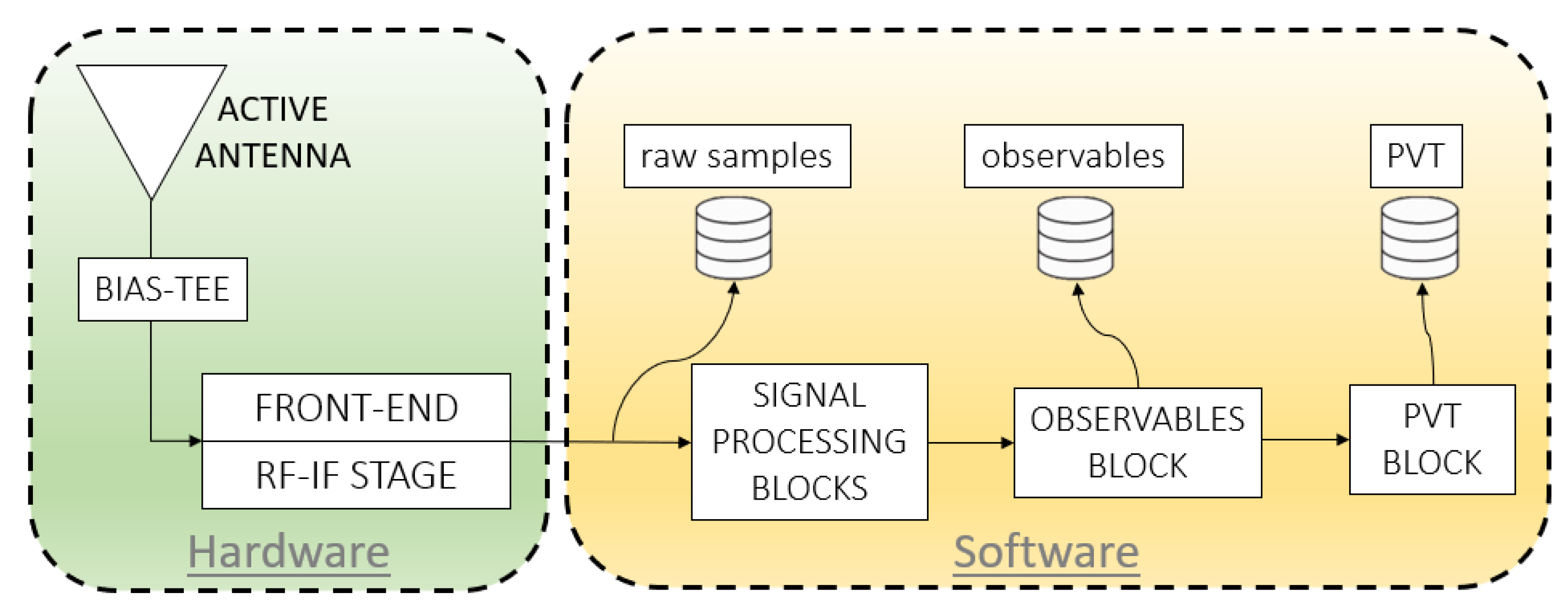
The most common architecture of a GNSS-SDR receiver is shown in
Figure 1. The front-end acquires the signal received by a proper GNSS antenna, demodulating it at an Intermediate Frequency (IF). Then, after the analog to digital conversion, the samples are fed to the signal processing chain that performs acquisition and tracking of the available satellites. The observables block-compute the code and carrier phase measurements, outputting the observables; lastly, the PVT block performs the Point Velocity and Time (PVT) computation. The quality of the clocks is fundamental, since they are used for the estimation of the propagation time. The PVT solution performance completely relies on clock measurements; indeed, space vehicles and receiver clocks must be as synchronized as possible with respect to the GPS time (GPST). GNSS satellites are equipped with very precise atomic clocks, while receivers, especially the low-cost ones, are often equipped with Temperature-Compensated Crystal Oscillator (TCXO) clocks that exhibit a noisy short-term stability and a poor long-term stability [
1]. The satellites’ clock offsets are corrected through parameters encapsulated in the navigation message broadcasted by the Ground Control Segment. The receivers’ clocks could not be corrected; thus, GNSS producers implemented some kind of clock-steering mechanism in order to maintain the receiver time within a certain range of the GPST and remove the receiver clock errors on a continuous basis.
SDR technology has evolved steadily over the decades following its birth in the mid-1980s, with various surges of activity being generally aligned with new developments in related technologies (processor power, serial busses, signal processing techniques, and SDR chipsets). Some important advances were achieved by Akos [
2] and Borre in [
3] following the SDR approach. Nowadays, there are some software solutions in GNSS positioning following this approach. Ledvina et al. proposed a twelve-channel real-time GPS L1 software receiver, achieving an accuracy of 10 m [
4]. A comprehensive list of the different GPS receiver architectures based on software-defined radio techniques are reported in [
5]. The PLAN research group from Calgary University developed GSNRx (GNSS software navigation receiver) [
6], focusing their study on the algorithm’s flexibility and processing efficiency using the Graphics Processing Unit (GPU), achieving centimeter-level positioning. In [
7], Munich University presented ipexSR, a real-time-capable software GPS/Galileo receiver along with a useful GUI (Graphic User Interface). The tests performed show an accuracy level better than 30 cm for code measurements and 1 mm for carrier phase measurements. In 2009, in [
8], Fantino et al. proposed N-Gene, a GNSS receiver completely designed in software, able to run in real-time on a common Personal Computer. A promising software receiver capable of acquiring, processing, and computing navigation solutions for different kinds of constellations (GPS, GLONASS, Galileo, and BeiDou) in different frequency bands (L1, L2, and L5) is GNSS-SDR, developed by CTTC (Centre Tecnològic de Telecomunicacions de Catalunya). A detailed description is provided by Fernandez [
9]. The source code released under the GNU General Public License (GPL) secures practical usability, inspection, and continuous improvement by the research community, allowing discussion based on tangible code and the analysis of results obtained with real signals [
9].
In the past years, few studies have focused on the relationship between GPS receiver clock errors and GPS positioning precision; in [
10], Bruggemann et al. presented a study regarding a theoretical CSAC (Chip Scale Atomic Clock) error model constructed and tested in a “clock coasting” application in airborne GPS navigation. The results achieved show that “clock coasting” with CSACs results in an improved Dilution of Precision (DOP) for up to 55 min under low satellite visibility or poor geometry in comparison with a typical crystal oscillator. In [
11], Li and Akos implemented a clock-steering algorithm in a software GPS receiver that maintains the receiver time within a certain range from the GPS time (GPST); the single-point and carrier-phase differential position solution results show that, when the steering option is turned on, the remaining clock errors in the receiver measurements are less than 50 ns. In [
12], Hee-Sung et al. proposed a compensation method to eliminate the effects of abrupt clock jumps appearing in low-quality GPS receivers. Experimental results based on real measurements verify the effectiveness of the proposed method. In [
13], Thongtan et al. estimated the receiver clock offsets according to three timescales: GPST, GLONASS time (GLONASST), and Beidou time (BDT). The estimated receiver clock offsets for static Precise Point Positioning (PPP) tests were around 32, 33, and 18 nanoseconds from GPST, GLONASST, and BDT, respectively. In [
14], Fernandéz et al. presented an analysis of the correlation between temperature and clock stability noise and the impact of its proper modeling on the holdover recovery time and on the positioning performance. They found that fine clock coasting modeling leads to an improvement in vertical positioning precision of around 50% with only three satellites; an increase in the navigation solution availability was also observed; a reduction of holdover recovery time from dozens of seconds to only a few could be achieved. Moreover, in [
15], with the aim of ensuring the stability and precision of real-time time transfer, Weijin et al. proposed an adaptive prediction model and a between-epoch constraint receiver clock model; the results with the between-epoch constraint receiver clock model were smoother than those with a white noise model, as the average root mean square (RMS) values were significantly less, by at least 50%. In [
16], Yiran et al. investigated the time-correlated error coupled in the receiver clock estimations, proposing an enhanced Kalman filter; the RTK positioning performance was increased by a maximum of 21.40% when compared with the results obtained from the commercial low-cost U-Blox receiver.
The clock-steering mechanism involves three concepts: Time tag, time offset, and clock bias. The time tag indicates the estimated time instant when the measurements are sampled by the receiver. The time tag is decomposed into an integer part and a non-integer part. The non-integer fractional part of the time tag is called the time offset. The clock bias corresponds to the deviation of the receiver time reference from the GPS time reference. The clock-steering methods are divided into two categories. One is continuous steering and the other is clock jumping. In continuous steering, the clock bias is monitored and controlled continuously by a feedback mechanism so that it can be bounded within small ranges. The continuous steering method is adopted by several high-quality geodetic-grade receivers. In clock jumping, the clock bias is monitored but not controlled. If the clock bias grows quickly in one specific direction and reaches a pre-defined bound, an large intentional clock jump is applied in the opposite direction to prevent further growth. At the same time, to nullify the clock jump effects in the clock bias, the same amount of jump, but in the opposite direction, is applied to the time offset. The clock-jumping method, in general, causes two different types of misalignment in relative differential positioning: Reception time misalignment (RTM) and transmission time misalignment (TTM). The RTM occurs when the time tags or the time offsets of the two receivers are not the same, which means that the time tags are not exact integers. Meanwhile, the TTM occurs when the clock biases of the two receivers are different [
12]. The correction mechanism of the receiver’s clock currently implemented in the GNSS-SDR expects that the PVT block sends a clock correction message to the observable block. This happens only if the receiver clock offset is greater than a certain threshold (default is 40 ms). This value was found to be reliable following the tests of Li and Akos, who stated in [
11] that if the receiver clock error is larger than 57 ms, the least squares solution will fail. If the receiver clock correction is enabled, then, in addition to this “gross” correction made by the PVT block, the RINEX observables are corrected by the computed clock correction value. The main aim of this work is the assessment of the performance of the Global Navigation Satellite Systems software receiver (GNSS-SDR), developed by CTTC (Centre Tecnològic de Telecomunicacions de la Catalunya). Particular attention was paid to the study of the clock-steering mechanism due to the low-cost characteristics of the front-end used. Different tests were carried out by employing a Software-Defined Receiver with steering either activated or turned off. In particular, following the work done in [
17], we want to evaluate the influence of the steering mechanism on the position solutions. The accuracy of the results of two different code positioning algorithms were analyzed, namely Single-Point (SP) and Code Differential positioning (DGPS).
2. Methodology
GNSS receivers, including those that are Software-Defined, provide four types of measurements: Pseudorange, Doppler, carrier phase, and carrier-to-noise through the RINEX format. The first three measurements are used to achieve receiver position [
18], while the carrier-to-noise density provides an indication of the accuracy of the tracked GNSS satellite observations and the noise density as seen by the receiver’s front-end [
19]. It also indicates the level of noise present in the measurements. The pseudorange measurement
P is expressed by the following relation [
20]:
where
is the geometrical distance,
is the receiver clock offset,
is the satellite clock offset,
T is the tropospheric delay,
I is the ionospheric delay,
is the code multipath,
is the delay due to the Sagnac effect, and
comprises the receiver hardware delays and receiver noise of the code measurements. Satellite clock offset correction parameters are transmitted in navigation data, while ionosphere delays were broadcasted and troposphere delays were estimated by using Saastamoinen model. In this study, we focus our attention mainly on the change in receiver clock offset when the clock-steering mechanism is enabled or not. In order to estimate clock offset together with receiver coordinates, at least four equations expressing the distance between an unknown receiver position and the known
ith satellite position are necessary. The equations can be linearized around an a priori value, obtaining:
where
(
n × 1) is the difference vector between the
n raw pseudoranges and a priori information (with
n GPS observations),
H (
n × 4) is the design matrix,
(4 × 1) is the state vector, and
is the residuals vector, which includes all unmodeled errors (measurement noise, multipath, and so on). The explicit forms of
H and
are:
where the superscript
n is the number of simultaneous GPS measurements and
is the a priori pseudorange of
n GPS satellites. The set of Equation (1) is solved for
by means of the Weighted Least Square (WLS) method, and the solution is given by the equation:
where W (
n ×
n) is the weighting matrix. It can be set as the inverse of the measurement covariance matrix
R, weighting the accurate measurements more and the noisy ones less. Here, all pseudorange errors are considered independent; thus, the covariance matrix is set equal to the identity matrix, with the weights calculated as a function of the satellite elevation angle.
The least square (LS) estimation is used to update the a priori value:
In this way, an estimation of the four unknown parameters was achieved.
3. Experimental Setup
The green box in
Figure 1 shows the simplest hardware configuration required to use a Software-Defined Receiver. In detail, it is made up of an active antenna, a bias-tee used to feed the antenna, and a front-end. The antenna employed in this experiment is a Topcon Geodetic PG-A1 antenna whose main characteristics are depicted in
Table 1. The front-end used is a Nuand bladeRF x40, a low-cost software-defined radio, able to tune from 300 MHz up to 3.8 GHz. The yellow box in
Figure 1 represents the all signal processing tasks running on the processing unit by means of the software. The Software-Defined Receiver chosen in this study is the GNSS-SDR. Is is an open-source project hosted on
github.com; it is written in C++, allows signal acquisition and tracking of the available satellite signals, decodes the navigation message, and computes the observables. A detailed description of the GNSS-SDR software can be found in [
9] and [
21]. The GNSS-SDR ran on a notebook equipped with an Intel i7 microprocessor with 16 Gb of RAM using a stable release of Ubuntu 16.04.
The GNSS-SDR allows the user to store both the intermediate frequency (IF) data and the RINEX files. In this experiment, we chose to use the latter strategy. The RINEX files obtained were post-processed by using Single-Point Positioning and Code Differential Positioning. The post-processing elaborations were carried out with the RTKlib package.
The GNSS-SDR allows the user to define a custom GNSS receiver, including its architecture (number of bands, channels per band, and targeted signal) and the specific algorithms and parameters for each of the processing blocks, through a single configuration file (a simple text file in INI format). Thus, each configuration file defines a different GNSS receiver [
22].
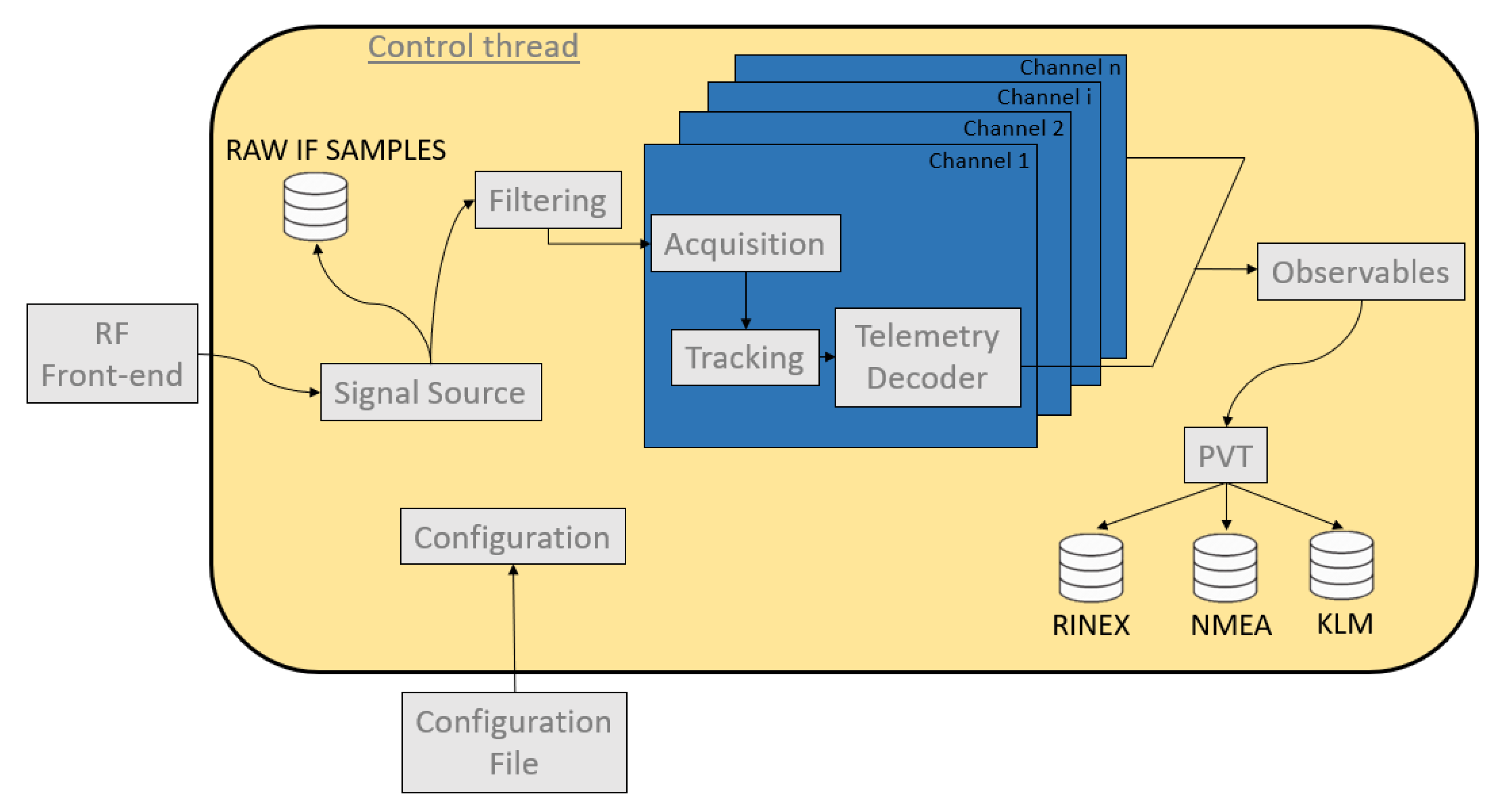
Figure 2 depicts the flowgraph generated by the software.
The Signal Source block is in charge of carrying out the communication between the hardware (front-end) and the software (GNSS-SDR) that will receive the raw samples from the analog-to-digital converter (ADC). The choice fell on the library OsmoSDR, which provides a software driver for several front-ends, including the bladeRF. The sampling frequency was set to 4 MSPS in order to also acquire the Galileo E1 signal, while a value of 48 dB for the IF gain was revealed to be the best compromise between lower values, which limits the signal reception, and higher values, which result in higher I-Q errors.
There is no need for filtering because the front-end already down-converts samples to baseband.
The Channels block creates a number of channels, and each of them encapsulates blocks for signal acquisition, tracking, and demodulation of the navigation message for each single satellite.
The role of the Acquisition block is the detection of the presence/absence of signals coming from a given GNSS satellite. In the case of a positive detection, it should provide coarse estimations of the code phase and the Doppler shift, yet accurately enough to initialize the delay and phase tracking loops [
22]. For the Acquisition block, we set the coherent integration time to 1 ms for GPS and 4 ms for GALILEO.
The role of the Tracking block is to follow the evolution of the signal synchronization parameters: Code phase, Doppler shift, and carrier phase. The implementations described below perform such estimations, which are assumed to be piece-wise constant within an integration time [
22]. The key parameters of the GPS’s tracking block are the Phase-Locked Loop (PLL) and Delay-Locked Loop (DLL) bandwidths, which we set here to 35 and 2 Hz, respectively.
We experienced that an important tracking parameter for the GALILEO is the , allowing the receiver to track the data-less pilot signal E1C, enabling an extra prompt correlator. For the GALILEO’s tracking block, the PLL bandwidth was set to 7.5 Hz, while the DLL bandwidth was set to 0.5 Hz.
The role of the Telemetry Decoder block is to obtain the data bits from the navigation message broadcast by GNSS satellites [
22]; the implementation of this block was set as shown below:
The role of the Observables block is to collect the synchronization data coming from all of the processing Channels, and to compute from them the basic GNSS measurements: Pseudorange, carrier phase, and Doppler shift [
22]. The GNSS-SDR performs pseudorange generation based on setting a common reception time across all channels [
23]. Actually, in the GNSS-SDR, there is a common Observables implementation suitable for all kinds of receiver configurations:
Lastly, the role of the PVT block is to compute navigation solutions and to deliver information in adequate formats for further processing or data representation [
22].
The parameters and allow users to obtain RINEX with custom rate frequencies. In this application, we set those parameters to obtain 10 Hz RINEX observations. The configuration files for the two tests that were carried out were the same, except for the parameter, which as set to false (steering off) for test 2.
Once the acquisition is completed, the GNSS-SDR stores different data outputs (RINEX .nav, RINEX .obs, .kml, and so on). We experienced that, in the software, when the acquisition targets multi-constellation signals but it receive signals from a unique constellation, it does not write the mixed ephemeris RINEX file (RINEX .P). This is a limitation of the current version of the software. For this reason, the satellite ephemerides were downloaded from the Crustal Dynamics Data Information System (CDDIS) site, in which the product archives of the Multi-GNSS Experiment (MGEX) projects are stored.
In order to investigate the performance of the hardware involved, we applied our analysis to the measurements captured in a strong multipath scenario in the Centro Direzionale (CDN) site (Naples, Italy). This is a difficult environment (as previously showed by the authors in [
24]) in which the receiver is surrounded by tall buildings, as depicted in
Figure 3. It can be seen as a typical example of an urban canyon, where many GNSS signals are strongly degraded by multipath effects or blocked by skyscrapers. Two different tests were carried out: In the first one, the clock-steering algorithm was activated, while in the second, it was disabled. The experiments were conducted on 6 and 7 November 2019. According to data products of the Space Weather Prediction Center of the National Oceanic and Atmospheric Administration (NOAA) of the United States Department of Commerce
ftp://ftp.swpc.noaa.gov/pub/warehouse/2019/WeeklyPDF/prf2306.pdf, the solar activity during the experiment was very low, with R, S, and G indexes considered null while the Kp index was 1. These space weather conditions imply that the errors due to the ionosphere ([
25]) during the experiment can be considered normal. Our interest is focused on the evaluation of SDR errors based on the activation or inactivation of the clock-steering mechanism; thus, in addition to the coordinates, the term
of Equation (
1) will also be analyzed relative to receiver clock offset.
So, for sake of clarity, the main features of the tests conducted in this paper are shown in
Table 2.
4. Results
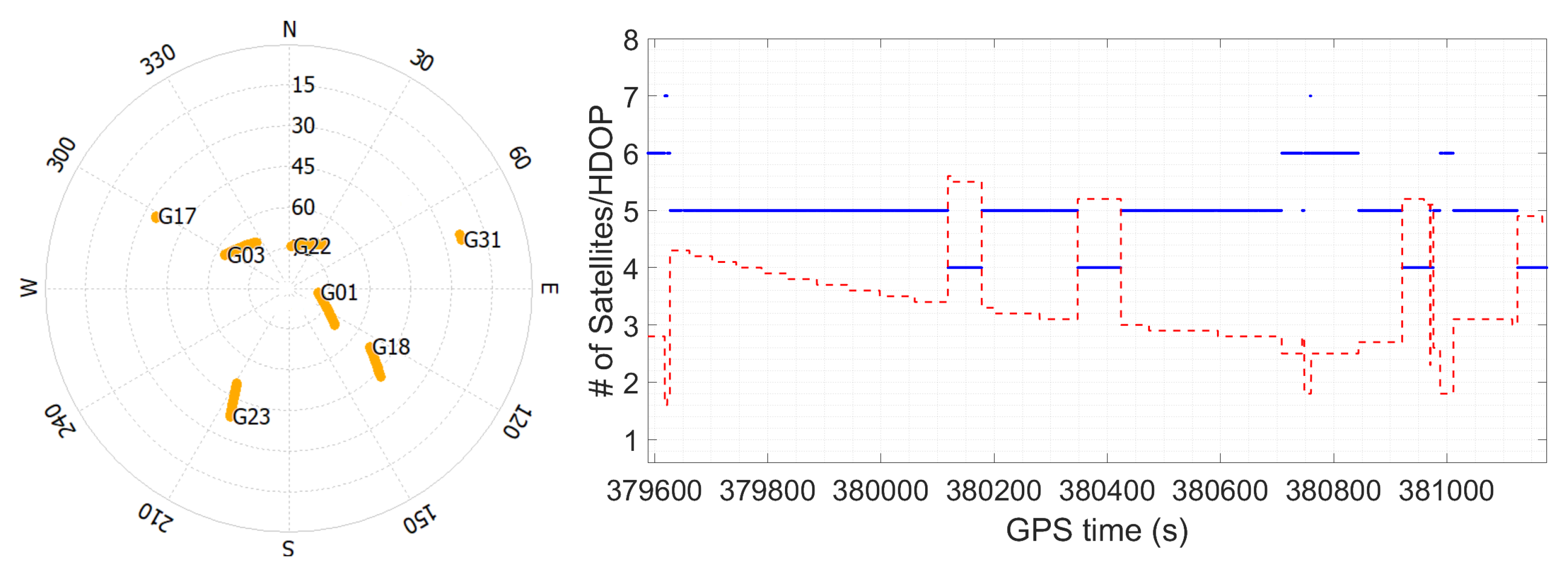
In
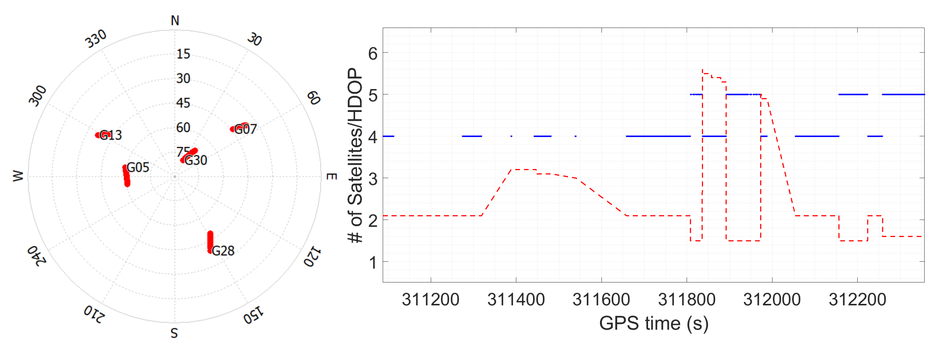
Figure 4, the skyplot and the Horizontal Dilution of Precision (HDOP) for test 1 (steering on) are shown. As depicted in the figure, the SDR, despite operating in a difficult environment, was able to track six GPS satellites, achieving an HDOP value of about 3. In
Figure 5, the skyplot and the Horizontal Dilution of Precision (HDOP) for test 2 (steering off) are shown. As depicted in the figure, the SDR tracked fewer satellites than in the previous test. However, a reliable comparison cannot be carried out because the data acquisition campaigns were not simultaneous.
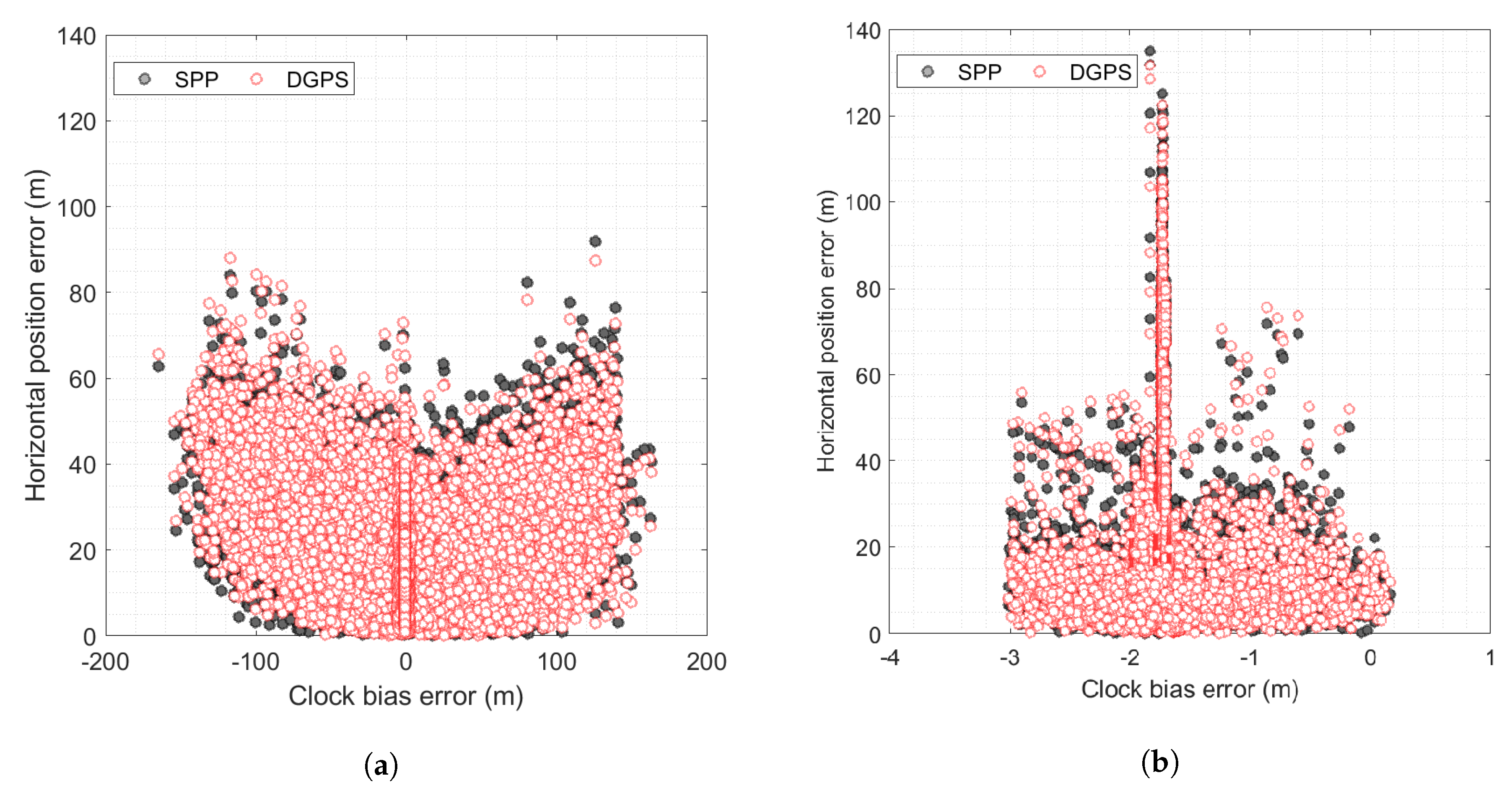
Figure 6 shows the error in estimates of a horizontal position versus the errors in the corresponding clock bias estimates for the three tests carried out. The scatter shows no apparent correlation between the two errors.
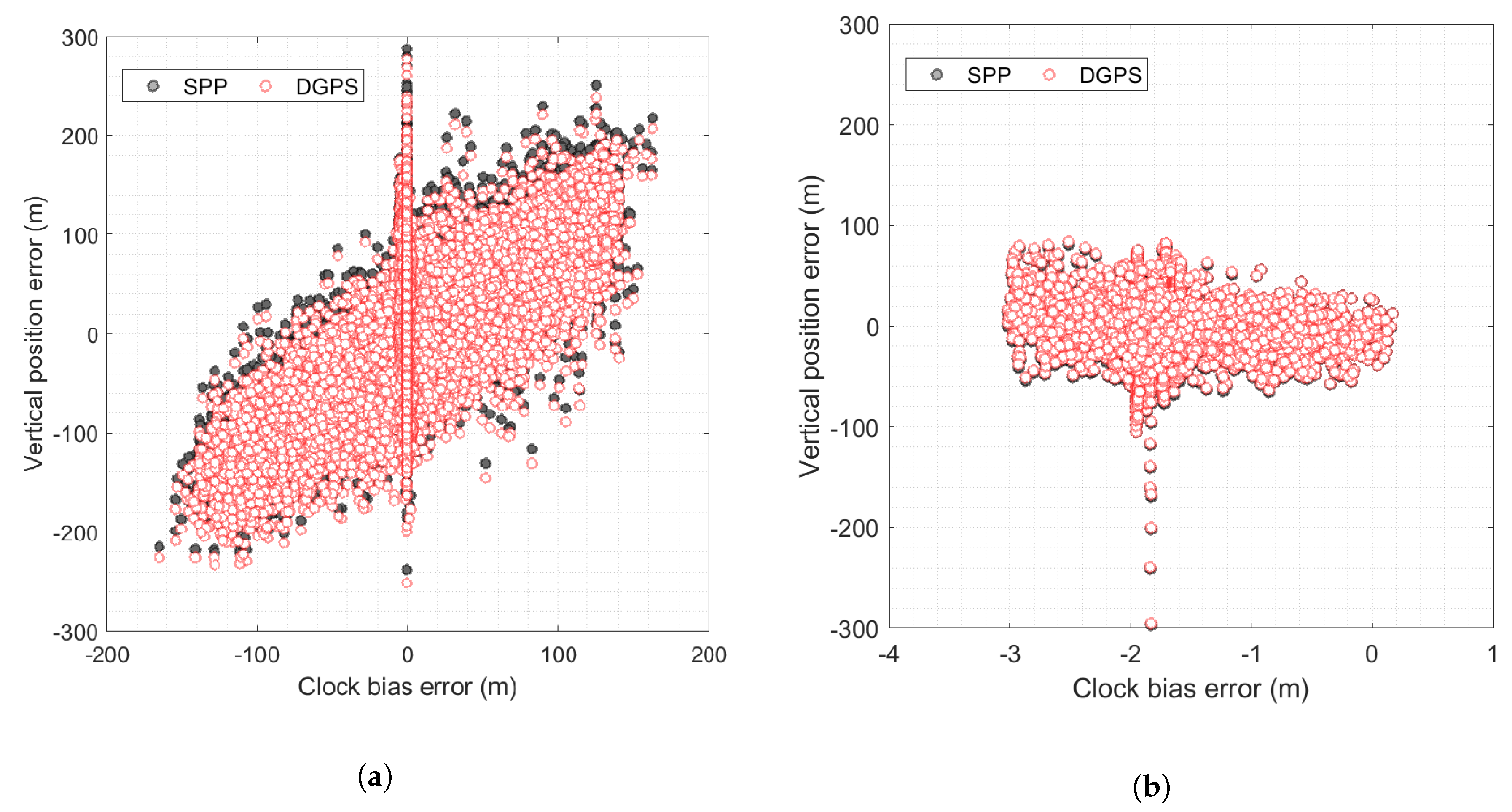
Figure 7 shows the error in estimates of a vertical position versus the errors in the corresponding clock bias estimates for the three tests carried out. In Panel (a), those values for test 1, the one with steering algorithm activated, are shown; a strong linear correlation can be observed. This is not a surprise; indeed, as noticed by Misra in [
26], a change in receiver clock bias changes all of the pseudoranges equally by a common amount. The effect of a change in user altitude is similar: All pseudoranges increase or decrease, but, in general, not equally; hence, the correlation.
This correlation cannot be noticed in Panel (b) and Panel (c), respectively showing the error in estimates of a vertical position versus the errors in the corresponding clock bias estimates for test 2 and test 3.
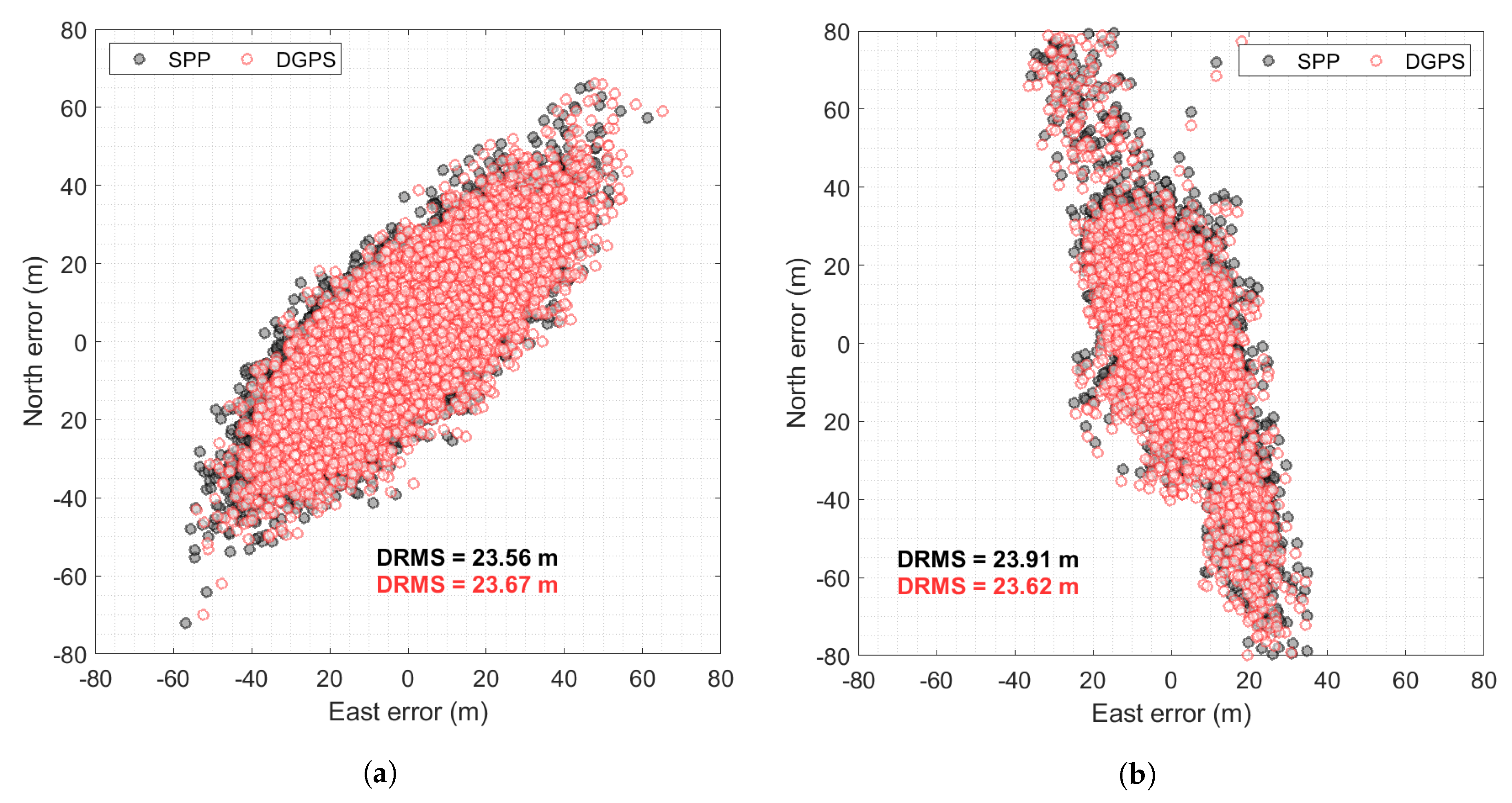
In Panel (a) of
Figure 8 is shown the scatter plot of the position errors of the Software-Defined Receiver with the three positioning modes carried out when the steering algorithm was enabled (test 1). Single-Point solutions (black markers) and Code Differential solutions (red markers) are quite similar, with about the same DRMS indicator. In Panel (b) of
Figure 8 is shown the scatter plot of the position errors of the Software-Defined Receiver with the three positioning modes carried out with the steering algorithm disabled (test 2). Like before, the Single-Point solutions (black markers) and Code Differential solutions (red markers) are quite similar.
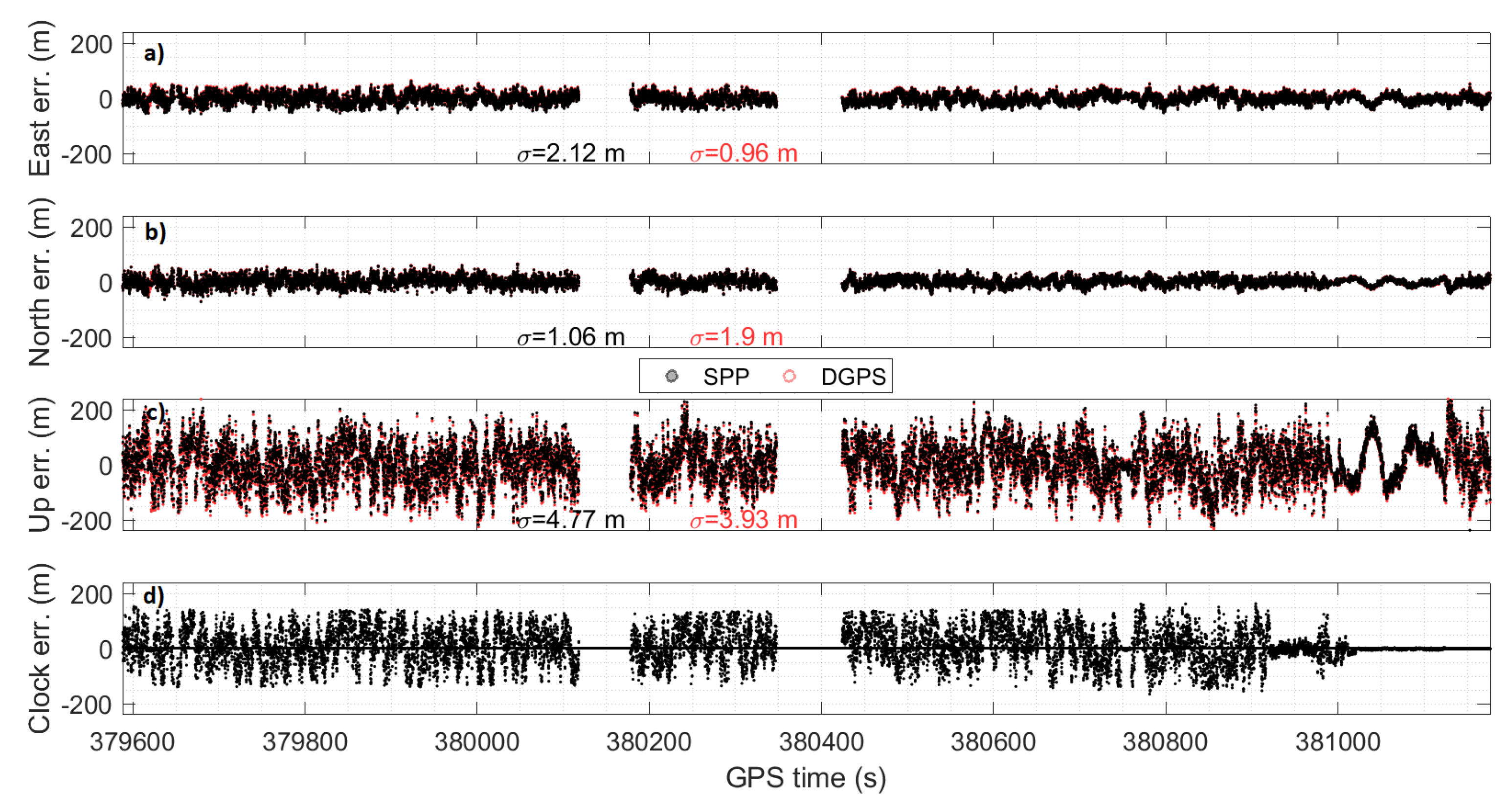
Figure 9 shows the position’s error components in the time domain and the clock bias error trend for test 1. The test’s results for the Single-Point solution achieved mean error components of 2.12, 1.06, and 4.77 m for the East, North, and Up components, respectively. The test’s results for the Code Differential solution achieved mean error components of 0.96, 1.90, and 3.93 m for the East, North, and Up components, respectively. On the bottom of
Figure 9, the clock bias trend is depicted, showing maximum and minimum values of 161 and −160 m, respectively.
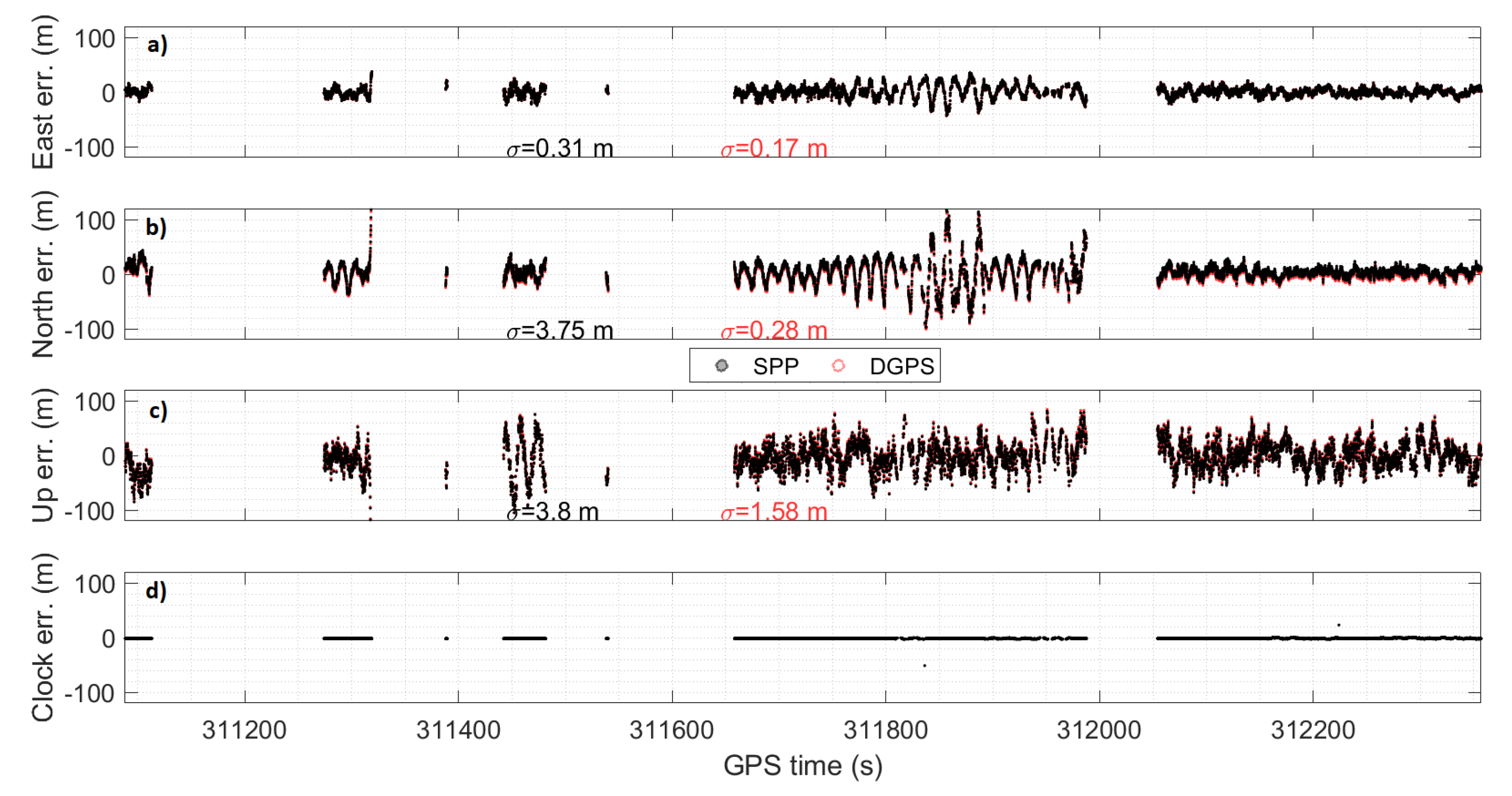
Figure 10 shows the position’s error components in the time domain and the clock bias error trend for test 2. The results of this second test for Single-Point solution achieved mean error components of 0.31, 3.75, and 3.80 m for the East, North, and Up components, respectively. The test’s results for the Code Differential solution achieved mean error components of 0.17, 0.28, and 1.58 m for the East, North, and Up components, respectively. On the bottom of
Figure 10, the clock bias trend is depicted, showing maximum and minimum values of 22 and −51 m, respectively.
6. Conclusions
In order to assess the GNSS-SDR’s performance, two tests were carried out, with steering either activated or turned off.
The activation of the steering mechanism allows one to obtain an improvement of the RMS on the East coordinate of about 8 m in both Single Point and in DGPS. Conversely, on the North coordinate, there is an opposite phenomenon with an increase of RMS of about 6 m. The combination of the two effects makes the DRMS quite similar in the two cases: 23.56 m when the steering algorithm is enabled versus 23.91 m when it is disabled in Single Point, and 23.67 m (steering on) versus 23.62 (steering off) m in DGPS. The real advantage in activating the steering mechanism is therefore not the achievement of a better planimetric accuracy, but the increase of solutions’ availability. The GNSS-SDR and, in general, the Software-Defined Receiver technology, although not new, has been revealed to be a promising technique, able to keep up with a scenario evolving as rapidly as the GNSS. Indeed, the key feature of this technology is the possibility of extreme customization, allowing the adaption of algorithms to new signals and to users’ needs. In this work, unfortunately, we were not able to use the ephemerides produced by the GNSS-SDR software due to the bug described above. The team of GNSS-SDR developers is working to solve it; therefore, our first future goal is to repeat the experiment using the navigation RINEX files generated by the software instead of those made available by the Multi-GNSS Experiment (MGEX) projects.
Another objective to be achieved in the next studies is to use a different front-end that allows to receive double-frequency data. This aspect is extremely important, as it will also allow us to analyze the effect of multipath on observables using the mp, a linear combination of dual-frequency code and phase measurements used to characterize the magnitude of the pseudorange multipath and noise for any GNSS system.


