Predicting the Saturated Hydraulic Conductivity of Clayey Soils and Clayey or Silty Sands

Abstract

Predictive models able to provide a reliable estimate of hydraulic conductivity can be useful in various geotechnical applications. Since most of the existing predictive methods for saturated hydraulic conductivity estimation are valid only for a limited range of soils or can be applied under certain restrictive conditions, a new method applicable to clayey soils and clayey or silty sands having a wide range of values of soil index properties is proposed in this study. For this purpose, 329 saturated hydraulic conductivity values, obtained by laboratory tests carried out on different soils, were collected in a database and used to develop five equations using a multiple regression approach. Each equation correlates the hydraulic conductivity with one or more geotechnical parameters. An equation was developed that predicts, within an order of magnitude, the saturated hydraulic conductivity in the range from 1.2 × 10⁻¹¹ to 3.9 × 10⁻⁶ m/s, based on simple geotechnical parameters (i.e., clay content, void ratio, plastic limit, and silt content).

1. Introduction

Hydraulic conductivity in cohesive soils is an important design parameter in various geotechnical applications, for example, when these materials are used as construction materials (e.g., in landfill, barrier systems, in levees, in earth dams, or in slurry walls), or in the cases where a modelling of filtration processes is required for the design.

Predictive models, able to provide a reliable estimate of hydraulic conductivity, can be useful during the screening phase, in order to restrict the number of field or laboratory permeability tests to perform in the design (time consuming and sometimes expensive) and to facilitate the choice of the most suitable soil for the execution of the earth works. Moreover, the methods to predict permeability could be used in preliminary numerical analyses.

Permeability predictive methods are generally based on soil index properties that are simple to be obtained by economic and routine classification tests. For this purpose, the literature presents several methods that allow predicting the saturated hydraulic conductivity (K_sat).

Predictive models can derive from empirical relationships, theoretical approaches such as capillary models and hydraulic radius theory [1] or from fractal models [2,3,4].

Different predictive methods for K_sat determination of plastic soils, use porosity (n), or void ratio (e), parameters related to grain size distribution (e.g., diameters corresponding to 10% and 50% passing in grain size distribution, d₁₀, d₅₀, % clay, or the specific surface) and Atterberg limits (e.g., liquid limit w_L or plasticity index IP). The different predictive methods refer to intact or remolded (homogenized) plastic soils or to compacted plastic soils [1].

Since most of the existing predictive methods for saturated hydraulic conductivity estimation are valid only for a limited range of soils or can be applied under certain restrictive conditions, a new method applicable to clayey soils and clayey or silty sands is proposed in this study. For this purpose, reliable information available in literature providing grain size distribution curve (GSDC), porosity or void ratio, Atterberg limits, and saturated hydraulic conductivity of different plastic soils are collected in a database, and used to develop an equation able to provide a reliable estimate of the saturated hydraulic conductivity for a wide range of soils using a multiple regression approach. Five equations were developed; each one correlates the hydraulic conductivity with one or more geotechnical parameters.

2. Existing Literature Methods to Predict K_sat

In the following, a set of equations proposed in literature by different authors to predict the K_sat value of plastic soils, are briefly summarized in chronological order.

The most widely used predictive method for K_sat estimation of both plastic and non-plastic soils is the use of the Kozeny-Carman equation [5], derived by semiempirical and theoretical evaluations and expressed by Equation (1):

$$K_{sat}=\frac{\gamma }{\mu }\frac{1}{\mathrm{C}}\frac{1}{{\mathrm{S}}_0^2}\frac{{\mathrm{e}}^3}{\left(1+\mathrm{e}\right)}$$

(1)

where γ and μ are the unit weight and the viscosity of fluid (when the permeant is water at 20 °C γ/µ = 9.933 × 10⁴ cm⁻¹·s⁻¹), C is a constant which depends on the porous space geometry (generally a value equal to 5 is assumed), S₀ is the specific surface per unit volume of particles (cm⁻¹), e is the void ratio. The determination of the specific surface is the main difficulty for the Kozeny-Carman equation application. For sand the specific surface can be calculated from grain size distribution [6,7,8], for plastic clayey soils it can be obtained with analytical methods or empirical correlations [9,10].

The Kozeny-Carman equation can be used for most soils having a single porosity [11] and should not be used for compacted soils which present a dual porosity [12]. Primary porosity corresponds to the fine structure at the micron scale of solid particles, the secondary porosity is equivalent to the porosity between artificially formed clay clods, which corresponds to a macrostructure resulting from excavation, transport, handling, and remolding by field equipment [8]. K_sat value in compacted soils is in large part influenced by this secondary porosity [1,8].

Another method for K_sat prediction was proposed by [13]. They proposed an experimental relationship, Equation (2), obtained by analysis of consolidation-test results:

$$e=\left(0.01\times I_p+0.05\right)\left(10+log{K}_{sat}\right)$$

(2)

where Ip is the plasticity index (%), e is the void ratio, K_sat is expressed in cm/s.

For remolded clay, the authors of [14,15] proposed Equation (3) for K_sat prediction in m/s:

$$K_{sat}=\frac{0.0174I_p^{-4.29}}{\left(1+e\right)}\left[e-0.027\left(w_p-0.242I_p\right)\right]$$

(3)

where e is the void ratio, w_p is the plastic limit (%), and I_p is the plastic index (%). The Equation (3) should be used with caution because it may predict negative K_sat values [1].

According to [16], K_sat values, determined in normally consolidated remolded clays, using Terzaghi’s consolidation theory, can be predicted through Equation (4):

$$K_{sat}=C\left(\frac{e^x}{1+e}\right)$$

(4)

where K_sat is expressed in m/s, e is the void ratio, x is equal to about 5 (or in a range of 3.97–6.39 according to [17]), and C is given by Equation (5):

$$C=0.00104I_p^{-5.2}$$

(5)

where I_p is the plastic index (%).

The authors of [18] proposed the correlation expressed by Equation (6) for predict K_sat in m/s knowing the void ratio (e) and the liquid limit (w_L in %). The experimental values of K_sat were determined in sand–bentonite mixtures (w_L > 50%) through oedometer tests using Terzaghi’s consolidation theory.

$$log{K}_{sat}=\frac{e-0.0535w_L-5.286}{0.0063w_L+0.2516}$$

(6)

For K_sat prediction, the authors of [10] proposed the correlation expressed by Equation (7) derived from the Kozeny-Carman equation. The equation was derived using results taken from the literature or obtained by the authors. The tests for K_sat determination were conducted on reconstituted (remolded) specimens under constant or falling head conditions, using rigid-wall permeameters and triaxial cells.

$$K_{sat}=C_P\frac{{\gamma }_w}{{\mu }_w}\frac{e^{3+x}}{1+e}\frac{1}{{\rho }_s^2{w}_L^{2\chi }}$$

(7)

K_sat is expressed in cm/s, C_P = 5.6 g²/m⁴, γ_w is the unit weight of water and equal to 9.8 kN/m³, μ_w is the water dynamic viscosity equal to 10⁻³ × Pa·s, χ = 1.5, ρ_s is density of solid expressed in g/m³, w_L is the liquid limit expressed in %, and the parameter χ is defined by Equation (8):

$$x=7.7w_L^{-0.15}-3$$

(8)

this relation is valid for plastic/cohesive (clayey) soils with 2.5 × 10⁻¹¹ cm/s ≤ K ≤ 3.8 × 10⁻⁶ cm/s (0.29 ≤ e≤ 5.96; 2.61 ≤ G_s (specific gravity of the solid particles) ≤ 2.87; 20% ≤ w_L ≤ 495%).

Examining in detail the Kozeny–Carman equation [1], the authors of [8] proposed Equation (9) which can be used for any soil, either plastic or non-plastic:

$$log\left(K_{sat}\right)=0.5+\log \left(\frac{e^3}{G_S^2{S}_S^2\left(1+e\right)}\right)$$

(9)

K_sat is expressed in m/s, S_S is the specific surface expressed in m²/kg and G_s, the specific gravity, is dimensionless. For non-plastic soil S_S (m²/g) can be determined by Equation (10) [8] when w_L is lower than 110%:

$$\frac{1}{S_S}=\frac{1.3513}{w_L}-0.0089$$

(10)

The authors of [19] proposed the following equation:

$$K_{sat}=7.2\times {10}^{-4}{C}_F^{-2}$$

(11)

where C_F is the clay content expressed in relative units and K_sat in m/day.

In [20], the authors proposed the following equation:

$$K_{sat}=\frac{6.31\times {10}^{-7}}{{\left(I_p-8.74p\right)}^{3.03}}{e}^{2.66{\left(I_p-8.74p\right)}^{0.234}}$$

(12)

where K_sat is expressed in m/s and p is the percentage of clay minerals in the soil divided by 100. This formula was derived knowing the hydraulic conductivity of five specimens, of expanding and non-expanding clays, determined in the laboratory using the falling-head test in an oedometer consolidation cell. Equation (12) is valid for fine-grained soils that contain non-swelling or limited-swelling clay minerals.

In [21,22], the authors proposed to evaluate K_sat from the Kozeny-Carman equation (Equation (1)) determining the overall soil specific surface per unit volume of particles S₀ combining the contribution of the plastic clayey fraction (d < 2 µm) and that of the coarse fraction (d > 2 µm) as expressed by Equation (13).

$$S_0=\frac{\left(S_{0,d >2\mu m}\times f_{d >2\mu m}+S_{0,d <2\mu m}\times f_{d<2\mu m}\right)}{f_{d >2\mu m}+f_{d <2\mu m}}$$

(13)

where S_{0,d> 2 µm} is the specific surface of the non-plastic fraction of soil, whereas the S_{0,d < 2µm} is the specific surface of the plastic clayey fraction, the f_{d > 2µm}and f_{d < 2 µm} are the related weight fraction corresponding to the diameters greater and lower of 2 µm [21]. Regarding the specific surface of the non-plastic fraction (d > 2 µm) of soil (S₀) it can be determined through the method of [23] expressed by Equation (14):

$$S_0=\frac{6}{D_{eff}}$$

(14)

where D_eff is the representative diameter expressed by Equation (15):

$$D_{eff}=\frac{100\%}{{{\displaystyle \sum }}^{\text{}}\raisebox{1ex}{$f_i$}\!\left/ \!\raisebox{-1ex}{$D_{ave,i}$}\right.}$$

(15)

f_i is the particles weight fraction, expressed in percentage, between two sieves of subsequent sieving. D_ave,i is the average diameter between the two considered sieves which can be calculated through Equation (16):

$$D_{\mathrm{ave},\mathrm{i}}=D_{l,i}^{0.404}\times D_{s,i}^{0.595}$$

(16)

D_l,i and D_s,i are the diameters of the larger and smaller between the two considered sieves.

Regarding the specific surface of the plastic fraction (d < 2 µm) of soil it can be determined through Equation (10).

Table 1. Types of soils and limitations of predictive methods for K_sat estimation.

Equations	Type of Soil	Limitations or Conditions of Validity
2	Clay	-
3	Remolded clay	May predict negative Ksat values
4	Normally consolidated remolded clay	x can vary in a range of 3.97–6.39
6	Clay	wL 50%
7	Plastic soils	2.5 × 10−11 cm/s Ksat ≤ 3.8 × 10−6 cm/s 0.29 ≤ e ≤ 5.96 2.61 ≤ Gs ≤ 2.87 20% ≤ wL ≤ 495%
9	Clay	wL < 110%
11	Sandy-clay soils	-
12	Clay	Soils that contain non-swelling or limited-swelling clay minerals
1 and 13	Clayey and silty-sandy soils	1 × 10−11 m/s ≤ Ksat ≤ 5 × 10−6 m/s

summarizes the types of soils to which the methods above described can be applied and the possible limitations or conditions of validity.

3. K_sat Database from Literature Review

From literature review, 329 saturated hydraulic conductivity values, determined by laboratory tests [17,21,24,25,26,27,28,29], were collected. The main geotechnical characteristics of the soils studied by different authors are shown in

Table 2. Main geotechnical characteristics of tested soils [17,21,24,25,26,27,28,29].

Reference	Numberof Tests	e (-)	IP (%)	wL (%)	CF (%)	SF (%)	Ksat (m/s)
[24]	9	0.6–1.8	38	68	80	20	3.8 × 10−11–1.1 × 10−9
[25]	49	0.33–1.12	2–62	19–91	14–75	16–64	2.7 × 10−11–2.7 × 10−9
[26]	32	0.31–1.39	11–46	24–70	16–65	25–58	1.3 × 10−11–3.3 × 10−10
[27]	40	0.52–1.00	12.5	17.5	2.7–5.7	43–70	1.2 × 10−7–3.9 × 10−6
[28,29]	22	0.69–3.84	18–71	43–119	47–77	23–56	1.3 × 10−10–4.0 × 10−9
[17]	63	0.53–1.86	9.5–25	37–74	5–35	38–88	1.2 × 10−11–6.8 × 10−8
[21]	114	0.33–1.21	5–45	17–70	5–67	32–84	1.2 × 10−11–9.3 × 10−8

e = void ratio; I_P = plastic index; w_L = liquid limit; C_F = clay fraction (d < 0.002 mm); S_F = silt fraction (0.002 < d < 0.06 mm); K_sat = saturated hydraulic conductivity.

.

The clay tested by [24] was a grey marine plastic Champlain Sea clay from Louiseville (Quebec). IP is 38%, w_L is 68%, and C_F (percentage of particles smaller than 2 µm) is 80%. The tests (No. 9) were carried out on an oedometer cell using the same specimen at different values of e, the hydraulic conductivity was determined through the falling-head permeability method.

The soils studied by [25] were compacted soil liners derived from landfills located in North America. Hydraulic conductivity was determined on “undisturbed” specimens (No. 49) taken using thin wall sampling (Shelby) tubes or as blocks. Hydraulic conductivity tests were performed in flexible-wall permeameters, rigid-wall Shelby tube permeameters, or consolidation cells equipped for direct measurement of hydraulic conductivity. The specimens have an I_p between 2% and 62%, a w_L between 19% and 91%, and C_F between 14% and 75%.

The authors of [26] studied 13 soils using three different compactive efforts (modified Proctor, according to ASTM D 1557, standard Proctor, according to ASTM D698, and reduced Proctor) and 32 specimens, compacted at a molding water content near to saturation, were considered for the database definition. The specimens have an I_p between 11% and 46%, a w_L between 24% and 70%, and C_F between 16% and 65%. The hydraulic conductivity of the specimens was determined by flexible-wall permeameters using the falling-head method according to ASTM D5084 procedure.

The 40 specimens studied by [27] were homogenized tailing from hard rock mines which can be identified, using the Unified Soil Classification System (USCS), as sandy silts of low plasticity (ML). The authors investigated four types of sulphide-free tailings obtained from three different sites. The soils have an IP equal to 12.5%, a w_L of about 17.5%, and C_F between 2.7% and 5.7%. The hydraulic conductivity was determined by means of rigid-wall permeameter using constant head and falling head conditions.

The 22 specimens investigated by the authors [28,29] were soils from Singapore, Bangkok, Ariake, Pusan, Tokyo, and London. The I_p values ranges between 18% and 71%, w_L between 43% and 119%, and C_F between 47% and 77%. Oedometer tests were carried out for hydraulic conductivity determination.

The 63 specimens investigated by [17] were remolded fine-grained soils having I_p values between 9.5% and 25%, w_L between 37% and 74%, and C_F between 5% and 35%. Hydraulic conductivity was determined by the falling head method in the standard one-dimensional consolidation apparatus.

The 114 specimens, studied by the authors of [21], were taken from the bottom and the walls of landfill, from road embankments, and from clay quarries of Italian sites. According to the USCS Classification (ASTM D 2487), the specimens considered by the authors are clayey sand and silty sand (SC-SM), silty clay (CL-ML), silt (ML), silt of high plasticity (MH), and clay of high plasticity (CH). The soils have I_p between 5% and 45%, w_L between 17% and 70%, and C_F between 5% and 67%. The hydraulic conductivity was mainly determined in triaxial test, according to the procedure ASTM D 5084-00 using the constant head method, on undisturbed specimens or remolded.

As can be observed from Table 2, the investigated soils have an I_P between 2% and 71%, w_L between 17.5% and 119%, C_F between 2.7% and 80%, and S_F between 16% and 88%. Therefore, a large range of soils was investigated, and it includes soils having low, medium, and high plasticity.

4. A New Predictive Method for the K_sat of Fine Grained and Plastic Soils

A new method able to predict K_sat of fine grained and plastic soils for a range of values larger than that considered by most of the existing literature methods, is formulated in this study.

According to [1], a reliable predictive method should take into account the following information: (i) the porosity n or the void ratio e; (ii) parameters referred to grain size distribution curve (GSDC) or specific surface of the solid grains; (iii) tests performed on fully saturated specimens; (iv) hydraulic conductivity of specimens determined through tests where the parasitic head losses can be excluded by using lateral manometers or proven to be negligible (for examples tests carried out in oedometer or triaxial tests for cohesive soils); (v) considering specimens that are not prone to internal erosion. Regarding the latter information, it is necessary to ascertain that the soil is not prone to internal erosion [30]. Regarding the soil grain size distribution, soils that have a grain size distribution that presents a concave upward curve, a gap inside the curve (gap-graded soils), or a broadly graded curve are generally considered to be internally unstable [31]. Different criteria can be used to determine the potential internal instability of a granular soil subjected to seepage [31,32,33,34,35,36].

Considering the information provided by [1] and the large number of experimental data contained in the created database (Table 2), five equations were developed in this regard for K_sat prediction using a multiple regression approach.

Among the different variables available, some of these were selected, according to their greater influence on the hydraulic conductivity.

The variables predicting the experimental value of the saturated hydraulic conductivity were progressively added to the equations in order to obtain the best correlation between the predicted value (K_pre) and the experimental one (K_exp).

The reliability of each of the five proposed equations was checked through a “Correlation Index” (CI), an index introduced by the authors and defined by Equation (17) which expresses how the predictive value of permeability (K_pre) approaches the determined one (K_exp):

$$CI=\frac{{{\displaystyle \sum }}^{\text{}}{\left[ln\left(\frac{K_{exp}}{K_{pre}}\right)\right]}^2}{n}$$

(17)

where n is the number of soils. The best correlation is represented by a CI value tending to zero.

The equations proposed in this study for K_sat prediction in m/s are summarized below together with the CI values.

$$K_{pre}=7\times {10}^{-6}{C}_F^{-2.898},CI=0.75$$

(18)

$$K_{pre}=1.498\times {10}^{-5}{C}_F^{-2.898}\times e^{2.9015},CI=0.46$$

(19)

$$K_{pre}=8.58\times {10}^{-4}{C}_F^{-2.898}\times e^{2.9015}\times w_p{w}_p^{-1.377},CI=0.33$$

(20)

$$K_{pre}=3.38\times {10}^{-2}{C}_F^{-2.898}\times e^{2.9015}\times w_p^{-1.377}\times S_F^{-0.921},CI=0.31$$

(21)

$$K_{pre}=7.22\times {10}^{-4}{C}_F^{-2.898}\times S_F{}^{-1.43}\times w_p^{-0.567}\times {\exp }_{}^{0.0165w_L},CI=0.67$$

(22)

The variables considered from Equation (18) to Equation (21) were taken using the following order: the clay content (C_F) in percentage, the void ratio (e), the plastic limit (w_p) in percentage, and the silt fraction in percentage (S_F).

The CI values show as the C_F contribution gives a good estimate of the K_exp value (Equation (18)), the correlation significantly improves adding e (Equation (19)) and slightly improves adding w_p (Equation (20)) and S_F (Equation (21)).

Another equation (Equation (22)) that considers only parameters obtained by economic and routine classification tests is proposed. The variables included are C_F, S_F, w_p, and w_L in percentage (excluding e).

The CI value found for this equation (0.67) is greater than that obtained for Equation (21). This shows that e is an important parameter influencing hydraulic conductivity value. In fact, its use allows reducing the CI value and providing a more accurate assessment of the hydraulic conductivity.

The performance of the five Equations (18)–(22) is shown in Figure 1, Figure 2, Figure 3, Figure 4 and Figure 5 where the K_exp and K_pre values (m/s) are compared for the 329 investigated specimens.

The first equation (i.e., Equation (18)) was obtained by examining the possible correlations between the K_exp values and a certain index property of the different investigated soils. From this research, it was found that the parameter that most influences hydraulic conductivity is C_F and the best correlation was found through a power function as shown in Figure 6. This strong correlation between the clay content and the hydraulic conductivity, through a power function, was also suggested by [19], anyway the strong dependence to this parameter can be found in the equations proposed by the authors of [20,25,26] for hydraulic conductivity prediction.

The second parameter among those investigated (such as n, I_P, w_p, w_L, and S_F), which added to Equation (18) allows to significantly approach the experimental value of K_sat with the predicted one, is the void ratio. Most of the predictive models present in literature consider the variable e in their formulation (i.e., Equations (1),(3),(4),(6),(7),(9),(12)). This variable allows to correctly differentiate the permeability of the same specimens having different values of e (e.g., soils tested in [17,24,28,29]).

Starting from Equation (19), Equation (20) was obtained adding w_p contribution. The plastic limit w_p is the parameter that allows, better than w_L and I_p, to improve the previous correlation between K_pre and K_exp especially for sandy silts of low plasticity for which the K_sat values predicted by the previous equations (i.e., Equations (18) and (19)) were slightly underestimated. This parameter is not usually correlated to hydraulic conductivity in the predictive methods present in literature (only Equation (3) contains this parameter) where the parameters w_L and I_p are more common (see Equations (2),(4),(6),(7),(12)). For clayey soils the dependence of K_sat to w_L is usually expressed by means of the specific surface (e.g., Equations (1) and (9)) through Equation (10).

Finally, starting from Equation (20), Equation (21) was obtained by adding the silt content S_F, a parameter that is not usual in literature predictive equations, which allows obtaining a more accurate estimate of K_sat. Equation (21) has the main advantage to take into account most of the variables influencing hydraulic conductivity, with respect to the correlations existing in literature that consider a lower number of variables (see Equations (2),(3),(4),(6),(7),(9),(11),(12)).

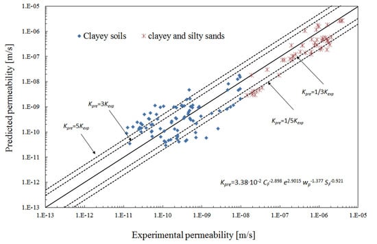
The variables considered in Equation (21) provide information about the grain size distribution (by means of C_F, and S_F), the mineralogical composition (by means of w_p) of the investigated soil as well as the void ratio (e). The model does not account only for anisotropic behavior and permeant characteristics (only water as permeant liquid).

As expected, Equation (21) suggests that an increase of C_F, w_p, and S_F values corresponds to an hydraulic conductivity decrease, whereas an increase of e results in an increase of hydraulic conductivity.

According to the results obtained by the application of the five equations, proposed in this study, it can be observed that parameters referred to GSDC and the porosity or void ratio of soil greatly influence hydraulic conductivity as also observed by [37]. In fact, the method proposed by the authors (Equation (21)) show the best predictive capacity among the five proposed equations.

The different methods summarized in Table 1 were applied, under the conditions imposed by each author, to the soils shown in Table 2 that refers to the laboratory permeability tests database. In particular, Equation (2) was not applied for sandy silts soils; Equation (3), valid for remolded clay, was applied for specimens investigated by [17] and negative values of K_pre were eliminated; the Equation (6) was applied only for soils having a value of w_L greater than 50%; the Equation (7) was not applied for soils having w_L lower than 20%; the equation 9 was not applied for sandy silts soils (i.e., soils investigated by [27]) and for soils having w_L greater than 110%; the Equations (4) and (12) were not applied to the created database since these methods are valid within a particular category of soils as shown in Table 1. The performance of these methods is shown in Figure 7.

The method of [18] (Equation (6), Figure 7c) shows a poor correlation and in particular underestimates the experimental values of K_sat as also observed by [1]. Additionally, the method of [19] (Equation (11)) shows a poor correlation and in particular, it overestimates the experimental values of K_sat (Figure 7f). The correlation improves with the method proposed by [14] and [15] (Equation (3), Figure 7b) but sometimes overestimates the experimental value of K_sat as also observed by [1]. The method proposed by [8] (Equation (9), Figure 7e) and by [13] (Equation (2), Figure 7a) shows a poor correlation for soils having hydraulic conductivity greater than 10⁻⁹ m/s. The method proposed by [10] (Equation (7)) shows a good predictive capacity but underestimates the hydraulic conductivity for soils having K_sat values greater than 10⁻⁸ m/s (Figure 7d).

The method that shows the best correlation between the predicted and experimental values of K_sat is the method proposed by [21] (Equations (1) and (13)) as can be observed in Figure 7g and from the CI value equal to 0.477. This method, as previously described, consists of the application of Kozeny–Carman formulation (Equations (1) and the application of Equations (13) for the determination of the specific surface area of the plastic soil fraction. The method takes into account most of the variables influencing hydraulic conductivity: the grain size distribution of soil, the specific surface (which is linked to w_L for plastic soils and therefore to the mineralogical composition), and porosity (n). In this method, the amount of particles with a diameter less than 2 µm greatly influences the hydraulic conductivity of plastic soils. As also pointed out by [21], their method is able to predict K_sat for a wide range of soils having hydraulic conductivity values ranging from 10⁻¹¹ to 5 × 10⁻⁶ m/s, in fact this method underestimates hydraulic conductivity of soils having K_sat values higher than about 10⁻⁶ m/s.

Equations (19)–(21) (CI ≤ 0.46) allow obtaining an estimate of K_sat slightly more accurate than that obtained by the application of the method proposed by [10] and by [21,22]. In particular, Equation (22), that considers only parameters obtained by economic and routine classification tests, provides predictive capacity slightly better than Equations (7) that needs e value.

The range of validity of the proposed equations includes soils having low, medium, and high plasticity and provides an accurate estimate of K_sat for soils having a wide range of values of soil index properties: I_P between 2% and 71%, w_L between 17.5% and 119%, C_F between 2.7% and 80%, and S_F between 16% and 88%.

5. Conclusions

In this paper, new equations for the saturated hydraulic conductivity (K_sat) prediction in clayey soils and clayey or silty sand were developed.

The equations were derived by empirical correlations using a great and reliable number of experimental data (No. 329) taken from literature [17,21,24,25,26,27,28,29] and related to the saturated hydraulic conductivity, grain size distribution curve, porosity or void ratio, and consistency limits of different soils. Five equations were developed; each one correlates the hydraulic conductivity with one or more geotechnical parameters.

The first equation considers the contribution of clay content (C_F), the second one adds the contribution of void ratio (e), the third adds the contribution of plastic limit (w_p), and the fourth adds the contribution of silt content (S_F). The correlation between the experimental and predicted values of hydraulic conductivity increases with the number of parameters considered in the equation. In particular, among these variables, C_F and e are the parameters that greatly influence the hydraulic conductivity value.

A fifth equation, which considers only parameters obtained by economic and routine classification tests (i.e., C_F, S_F, w_p, and the limit liquid w_L), is also proposed. The exclusion of the void ratio provides a less accurate prediction of the hydraulic conductivity compared to the fourth proposed equation that is able to estimate K_sat value in the range between 1/5 and 5 times the experimental value of K_sat.

The proposed method is able to predict K_sat of fine grained and plastic soils for a range of values (from 1.2 × 10⁻¹¹ to 3.9 × 10⁻⁶ m/s) larger than that considered by most of the literature methods.

The proposed equations can be very useful in different situations as modelling study or during a screening phase in order to restrict, for economic reasons and of time, the number of field or laboratory permeability tests.