Water Soil Erosion Evaluation in a Small Alpine Catchment Located in Northern Italy: Potential Effects of Climate Change

Abstract

Water erosion and evaluation of the average annual soil loss considering the potential effects of climate change are the focus of this study, based on the application of two empirical models, the RUSLE (Revised Universal Soil Loss Equation) and the EPM (Erosion Potential Method), to an Italian case study. A small mountain basin, the Guerna creek watershed, is located in the Central Southern Alps (Lombardy, Southern Alps, Bergamo), and it has been affected in the past by flooding and erosion events, which stressed the hydraulic weaknesses of the study area. Three different future climate scenarios were built for the middle of this century (from 2041 to 2060) on the basis of CORDEX data and Representative Concentration Pathways (RCP) set by the IPCC (Intergovernmental Panel on Climate Change) future scenarios: RCP 2.6, RCP 4.5, and RCP 8.5. As concerns climate, precipitation and air temperature are the variables used in the empirical models. On the other hand, potential effects on land use were also considered. Computed soil loss of 87 t/ha/year and 29.3 t/ha/year was achieved using the RUSLE equation and EPM method respectively, without considering the potential effects of climate change. The results achieved showed that climate change impacts on water erosion may not be negligible even by the middle of the current century (the annual average soil loss could change by 6–10% on a basin scale), and a major role is being played by seasonality in rainfall peak intensity.

1. Introduction

Soil erosion by water can occur at high rates in the alpine and pre-alpine environment, due mainly to its topographic, soil, and climate features. How these rates can change in the future climate is an important piece of information for developing and planning good management practices. A change in the climate may affect different factors contributing to the sediment yield and soil loss in mountainous areas.

Particularly, soil erosion is expected to be influenced by changes in air temperature, precipitation, and its distribution, which are impacting crop management and land use, plant biomass production, soil moisture, and the infiltration rate [1]. As a matter of fact, a close link between climate change and soil erosion can be observed. On the other hand, there are direct and indirect impacts that can increase or reduce soil erosion. The direct impacts are caused primarily by changes in rainfall amount, rainfall intensity, and rainfall spatio-temporal distribution. Precipitation patterns in different areas of the same continent or country can either rise or reduce in the future climate. This is also in line with the prediction of IPCC (Intergovernmental Panel on Climate Change) [2] for the precipitation changes worldwide. It is in fact likely to increase with increased rainfall amount, but it is not always dependent on the amount of rainfall. This means that soil erosion does not necessarily rise with increased rainfall amount, since rainfall intensity and its spatial distribution also affect soil loss significantly. In several studies, the increased frequency of intense rainfall events has been shown to result in an increase of soil loss, despite the predicted decrease of the amount of rainfall [1,3,4]. Ref [3] discovered that the impacts of precipitation intensity were greater than those of the number of rainy days. Ref [5] argued that the combination of changes in rainfall amount and rainfall intensity may have a greater impact rather than variations in any single factor. On the other hand, temperature rise is related to the indirect impacts on soil erosion [1,6]. Another important aspect to be considered is the effect of climate change on land use. One example of assessment of land use change scenarios was made in the Lo river basin (Vietnam). The land use change that was investigated in this area assumed the conversion of 20% of forest area into rice and agricultural crops and 15% of forest area into bushed, shrubs, and meadows. These cover soil variations showed a 28% increase of sediment load; then, it produced a significant effect on sediment production in the Lo basin [7,8]. Another example of land use impact on water erosion is given by [9], which predicted the variations of runoff and soil erosion in two catchments in Portugal during 2071–2100. They found an increase of erosion rates in the watershed covered by croplands and a reduction of erosion rates in the watershed covered by forest and vineyard lands. Therefore, afforestation is a method considered to be effective against soil loss under global change [1]. The last case study is the Carapelle watershed in Puglia (Southern Italy). Four different Best Management Practice (BMP) scenarios were implemented in the study area; the aim is to quantify soil erosion and to identify specific BMPs for reducing erosion. The investigation established that the BMP of reforestation provides the highest specific sediment reduction (ranging from 50% to 99%) and that winter wheat, which corresponds to the BMP (Best Management Practice) of contour farming, is the highest producer of sediment yield (between 0 and 63.8 t∙ha⁻¹∙year⁻¹) [10].

To this day, the climate change impact and the compensatory effects of different factors are still unclear and difficult to predict accurately. The most helpful and common way to predict soil erosion under climate change is the use of a modeling chain from climate models to basin hydrological models. There are different soil erosion models (empirical models, conceptual models, and physically-based models) that have been extensively used in these kinds of studies and that can be combined with climate models [11,12,13]. The RUSLE (Revised Universal Soil Loss) [14] and EPM (Erosion Potential Method) [15] methods are two of the most used empirical models to estimate soil loss by water erosion. These methodologies can produce valuable information on soil erosion processes and on their spatial distribution. They take into account the climatic parameters, topography, land use, and soil features of the study area and can support climate change impact analysis. Model outputs can be used to understand the impacts of future climate change. Different downscaling methods, such as statistical downscaling and dynamic downscaling, have been developed in order to move from the coarse spatial resolution of climate data to the finer one [16].

Over the years, also the climate scenarios have been developed from simple hypothetical scenarios to more realistic ones—for example, Special Report on Emissions Scenarios (SRES) families [17] and Representative Concentration Pathways (RCPs). The former and the latter were set in 2001 and 2013, respectively, by the Intergovernmental Panel on Climate Change [1]. In particular, concerning the alpine space, one example is the analysis of soil erosion trends in IPCC A2 and B2 scenarios [18], which were conducted by [19]. Another case study to be mentioned is [20], which examined the potential effects of climate change at a hydrological cycle within an Alpine river of Italy considering temperature and precipitation data generated via the IPCC SRES A1B, A2, and B1 [17].

The general aim of this research is an estimation of water erosion at the catchment scale and a spatial analysis of soil erosion trends in different IPCC scenarios. The RUSLE [14] and the EPM [15] methods are used. They are empirical models whose parameters can be estimated by laboratory investigations and by field observations and experiments. The most important climate variables in the RUSLE and EPM equations are precipitation and air temperature. The two models were applied to the study area, the Guerna creek watershed, which is a small mountain basin (A ≈30 km²) located in the Central Southern Alps (Lombardy, Bergamo). Interest in the Guerna basin arises from the need to evaluate sediment transport and sediment loss, which is manifested by the managing the body of Lake Iseo and the Oglio river, and because this watershed is exposed to hydrogeological risk. The two models were implemented in a Geographical Information System (GIS) supporting the management of the territorial database used to estimate relevant geomorphological parameters and to create different thematic maps [21].

In this analysis, three different climate change scenarios were considered in order to tentatively assess the impact on the water erosion and soil loss at the small basin scale. CORDEX data [22] were used. The EURO-CORDEX ensemble is based on the Representative Concentration Pathways (RCP) scenarios, that define pathways of the additional radiative forcing caused by anthropogenic activity till the end of the 21st century [23].

2. Material and Methods

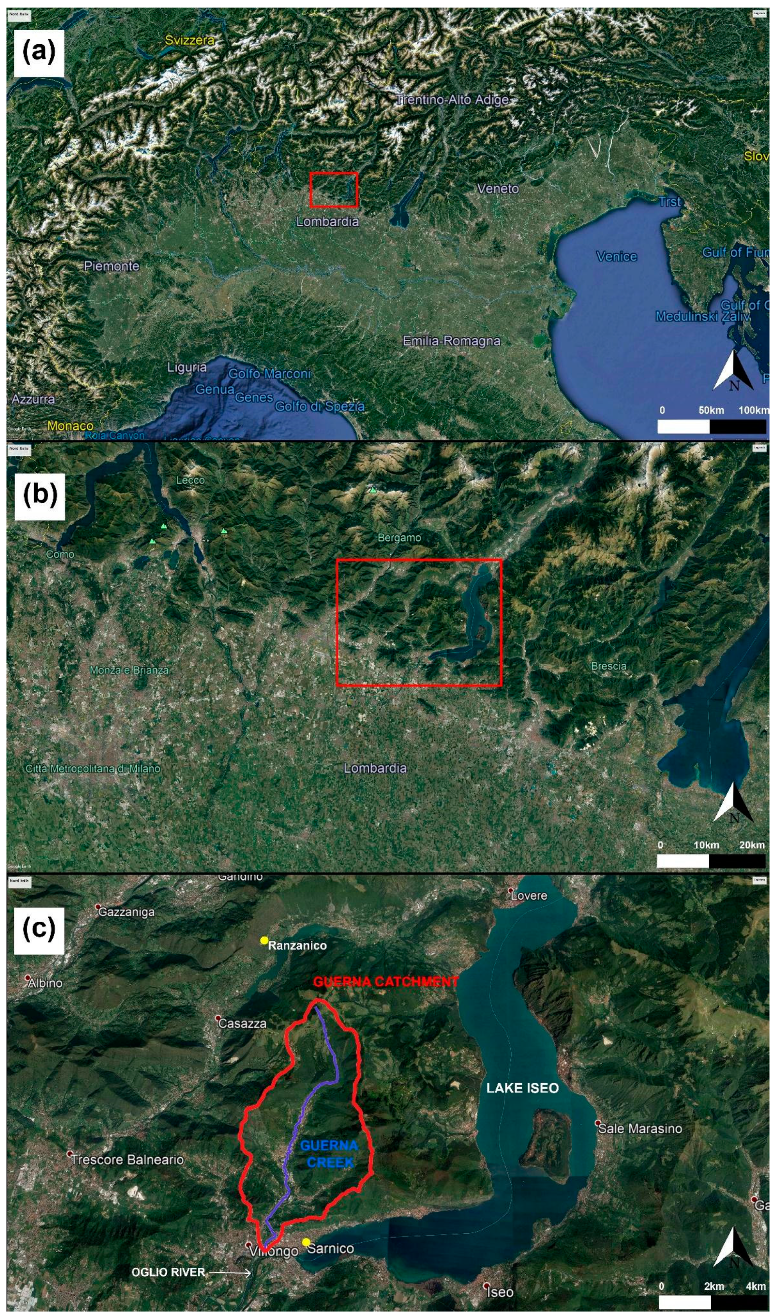
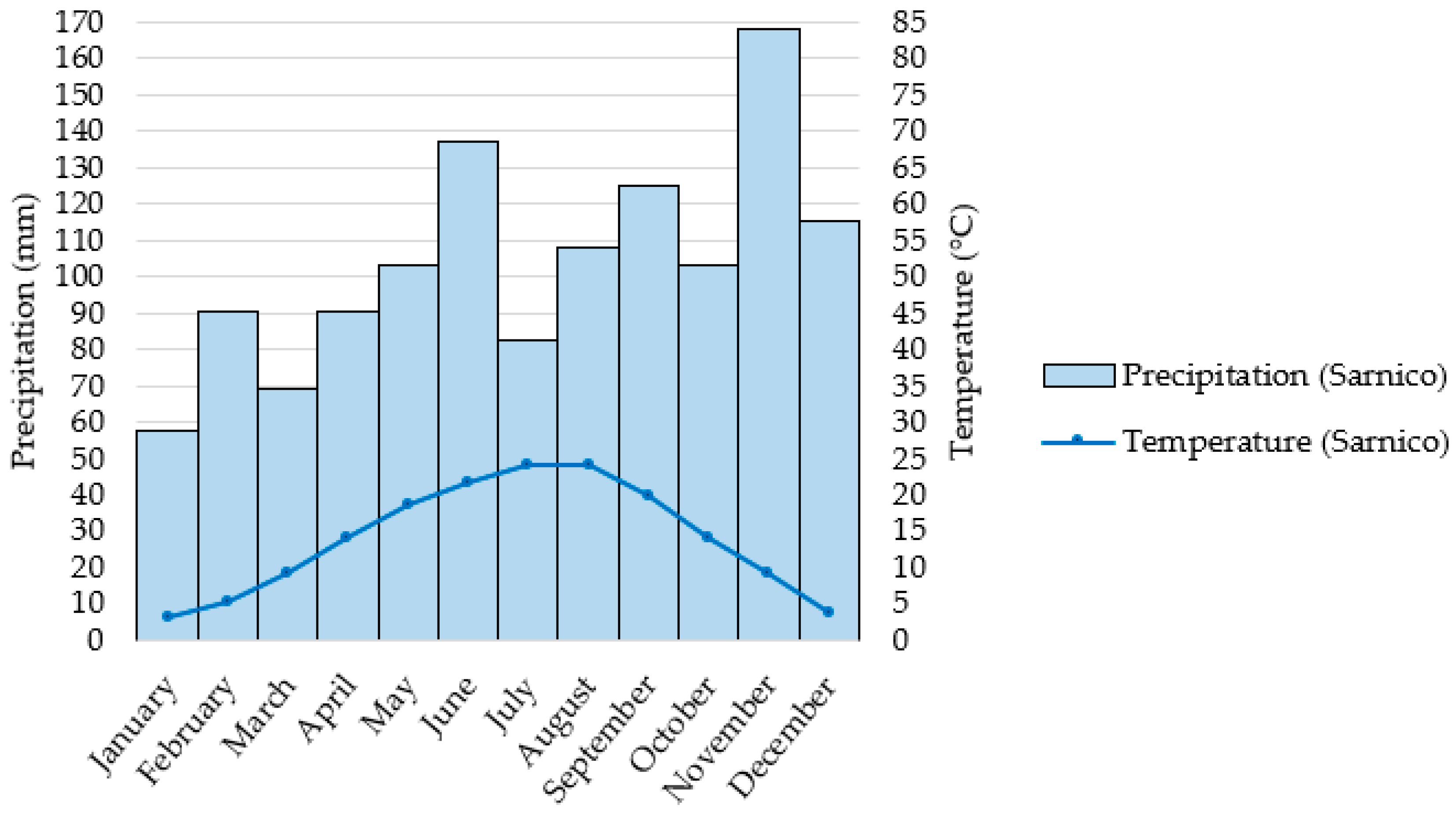
2.1. Study Area: The Guerna Catchment

The research was conducted in the Guerna creek catchment (Figure 1, where the catchment border was reproduced using shapefile on [24]), a small watershed located in the Province of Bergamo (central Italian Alps). The Guerna river springs from Monte Foppa at 1332 m a.s.l. and it is a right tributary of the Oglio river. The outlet of the catchment area is located at the confluence of the two rivers, a few meters downstream of the Sarnico dam (45.66 N, 9.94 E) controlling the water level in Lake Iseo. Most of the watershed surface belongs to the municipalities of Adrara S. Rocco, Adrara S. Martino, and Viadanica [21]. The main features of the Guerna creek and its watershed are reported in

Table 1. Main features of the Guerna creek basin.

Parameter	Value
Basin area [km2]	31
Wooded, reforested and forested area [km2]	20.5
Grassland [km2]	1.64
Agricultural area [km2]	6.00
Orchard and vineyard [km2]	1.07
Urban area [km2]	1.83
Bare areas [km2]	0.05
Average hillslope of the catchment area [%]	51
Maximum elevation [m a.s.l.]	1332
Minimum elevation [m a.s.l.]	185
Length of the main channel (Guerna creek) [km]	12.3
Longitudinal average slope of the main channel (Guerna creek) [m/m]	0.07
Mean annual precipitation at Sarnico station (years 2008–2011) 1 [mm]	1250.6
Mean annual temperature at Sarnico station (years 2008–2011) 2 [°C]	13.9

¹ This value was calculated by using available 4-year semi-hourly rainfall records provided by Consorzio dell’Oglio [25]. ² This value was calculated by using available 4-year daily temperature records provided by the regional agency for environmental protection ARPA Lombardia [26].

.

The Guerna creek was affected in the past by flooding and erosion events, which stressed the hydraulic weaknesses of the study area. Therefore, this watershed is exposed to hydrogeological risk because of, for example, poor cleaning of the water courses, abandonment of the territory, or disuse of agricultural practices (e.g., terracing, crops according to level curves, buffer strips, subsoiling, crop rotation, and intercropping). Sediment yield by the Guerna watershed is settling at the confluence with the Oglio River, right downstream of the Sarnico dam, making water management operations more complex.

The considered time window to estimate the mean annual precipitation and temperature in Sarnico (Table 1) is relatively short because of the limited semi-hourly rainfall records available that were used to calculate the R factor as described in Section 2.2 and Section 2.4. Nevertheless, the mean monthly precipitation and temperature values calculated and reported in Figure 2 retract the characteristic pattern of wet areas of the Southern Alpine range: two main rainfall peaks in late spring and in autumn with no dry season (as in the Alpine sublitoranean climate [27]), and a secondary peak during late summer, which is characteristic of the Alpine piedmont areas. For a more detailed report on the local climatology, see [28].

Ref [21] contains different thematic maps of the Guerna watershed created in a GIS environment (slope map, lithological map, hydrogeological instability map, and land use map). The lithological map in [21] reveals the presence of limestones, marly limestones, and flint limestones in most of the territory. In the Guerna mouth there are gravel, sand, blocks, and ferritization silt. The results of particle analysis of two soil samples (taken in the northern and in the southern part of the study area) by wet sieving and sedimentation [21] show the following information (

Table 2. Results of the particle analysis.

Sample Location of the Study Area	Xsk (%) 1	fi (%) 2			Soil Texture
		Clay	Silt	Sand
Southern part	46.68	22.90	38.48	38.62	Loam
Northern part	12.19	24.52	36.18	39.31	Loam

¹ Skeletal fraction (>2 mm) as a percentage on the total weight. ² Soil fraction, as a percentage on the weight passing at 2 mm diameter (according to USDA classification).

):

The hydrogeological instability map in [21] shows different sites characterized by landslides, alluvial cone, debris or terrigenous cover, rill erosion, and gully erosion. Nevertheless, most of the area of the catchment is without visible erosion effects, and it is mainly occupied by undergrowth and crop fields. Table 1 contains a detailed description of different soil use in the study area, as shown in the land use map in [21]. Table 1 also includes the average hillslope of the catchment, which was derived in a GIS environment from the slope map in [21]. This map reveals that lower slope values are mainly in the southern part of the study area, close to the Guerna mouth.

2.2. Empirical Models

The two empirical approaches that were adopted here for the computation of sediment loss at the basin scale are the RUSLE model [14] and the EPM method [15].

Both the RUSLE and EPM methods have limitations and shortcomings. The aim of the RUSLE methodology is to estimate water erosion in agricultural areas; therefore, the approach is not expected to be well suitable for erosion assessment in mountain catchments [29]. Moreover, the RUSLE equation does not consider the sedimentation processes, it tends to over-estimate soil loss, and it is not able to simulate gully erosion, mass movements, and riverbed erosion. Hence, the application of RUSLE over the alpine territory could present huge difficulties, due also to data availability problems [19]. The EPM equation describes the complex soil erosion mechanism by merely multiplying different factors. As a consequence, important aspects of the phenomenon such as sediment deposition and sediment routing are not taken into account. Additionally, the Gavrilovic model estimates mean annual erosion, while having very low accuracy on individual flooding events, where most of the sediment load is transported, especially at Mediterranean catchments [30]. Despite these deficiencies and shortcomings, the RUSLE and the EPM methodology can produce valuable information on alpine soil erosion processes and on their distribution. Indeed, they are two of the most used models, and their objective was the assessment of the soil erosion in relation to climate change; therefore, as suggested by [19], their analysis should be considered comparative and not absolute [21].

The RUSLE model is represented by the following equation [14]:

$$\mathrm{A}=\mathrm{R}·\mathrm{K}·\mathrm{LS}·\mathrm{C}·\mathrm{P}$$

(1)

where A is the computed soil loss (t∙ha⁻¹∙year⁻¹), R is the rainfall–runoff erosivity factor (MJ∙mm∙ha⁻¹∙h⁻¹∙year⁻¹), K is the soil erodibility factor (t∙ha∙h∙ha⁻¹∙MJ⁻¹∙mm⁻¹), LS is the topographic factor combining slope length L and slope steepness S, C is the cover-management factor, and P is the supporting practices factor.

The methodology applied in computing the RUSLE factors is the same used in [21] to simulate the sediment production in the years 2008–2011, using semi-hourly rainfall data that were recorded at Sarnico station. Therefore, the R factor and the K factor were considered uniform in the study area, whereas the LS, P, and C factors were calculated considering a spatial variability in the study area.

The R factor was estimated taking into account kinetic energy in a single rainfall and the rainfall intensity [31,32] during the available 4-year time series (from 2008 to 2011), where every rainstorm was considered as an erosive event, and several meaningful erosive events were collected. In fact, high values were obtained for the climatic factor for each year. Therefore, even if the series is short, a set of meaningful erosive events was sampled. Furthermore, this amount of meaningful erosive events in a short period stresses the importance of this basin as a hydrogeological risk-prone area. Both [33,34] created rainfall erosivity maps for a large area (respectively in Italy and in the world). The authors used data collected in different rainfall stations and, in some cases, the period covered by the time series is 5 years. The R factor was considered constant in the study area because it is a mountain area of limited extension, and there is only one rain gauge providing the daily rainfall data to estimate this factor.

The K factor was evaluated using equations in [35], which were proposed by [36] and revised in [37], and the results of the particle analysis reported in Table 2. The values obtained from the analysis of the soil samples, which were taken at different points of the watershed, were very similar; therefore, the K factor was considered constant in the area under investigation.

The LS factor was estimated modifying Moore and Burch’s equation [38] and using Nearing’s formula [39] and considering its spatial variability. The LS factor map was created in a GIS environment on the basis of the slope map of the flow accumulation map, as described in [21].

Average literature values were used for C and P factors, as described in [22,23].

The EPM method is the following [15]:

$${\mathrm{W}}_{\mathrm{sp}}=\mathrm{T}·\mathrm{H}·\mathsf{\pi }·\sqrt{{\mathrm{Z}}^3}$$

(2)

where ${\mathrm{W}}_{\mathrm{sp}}$ is the average annual specific production of sediments (m³∙km⁻²∙year⁻¹), $\mathrm{H}$ is the mean annual amount of precipitations (mm), $\mathrm{T}$ is the temperature coefficient (Equation (3)), and $\mathrm{Z}$ is the coefficient of erosion (Equation (4)).

$$\mathrm{T}=\sqrt{\frac{\mathrm{t}}{10}+0.1}$$

(3)

$$\mathrm{Z}={\mathrm{X}}_{\mathrm{a}}·\mathrm{Y}·\left(\mathsf{\phi }+\sqrt{\mathrm{i}}\right)$$

(4)

where $\mathrm{t}$ represents the mean annual temperature (°C), ${\mathrm{X}}_{\mathrm{a}}$ is the land use coefficient, $\mathrm{Y}$ is the coefficient of soil resistance to erosion, $\mathsf{\phi }$ is the coefficient value for the observed erosion processes, and $\mathrm{i}$ is the average land slope (m/m).

The average annual production of erosional sediments in the catchment area ${\mathrm{W}}_{\mathrm{g}}$ [m³∙year⁻¹] is the product between surface area $\mathrm{A}$ in km² and the weighted averaged annual specific sediment production ${\mathrm{W}}_{\mathrm{sp}}$:

$${\mathrm{W}}_{\mathrm{g}}=\mathrm{A}·{\mathrm{W}}_{\mathrm{sp}}.$$

(5)

The methodology applied in computing the EPM parameters is the same used in [21] to simulate the sediment production in the years 2008–2011, using semi-hourly rainfall data and daily temperature data that were recorded at Sarnico station. Therefore, the mean annual amount of precipitation was considered uniform over the entire study area. The coefficient of erosion and the temperature coefficient were calculated in a GIS environment, taking into account a spatial variability in the watershed. Indeed, the values used to estimate the coefficient of erosion Z have a spatial variability according to [21]. A linear trend of temperature as a function of altitude was assumed in order to estimate the temperature coefficient (T).

Different climate change scenarios were considered in order to tentatively assess the impact on water erosion on a small catchment scale, applying the two empirical models mentioned above. The computed soil loss (A) in the RUSLE model was estimated by solving Equation (1) but changing the rainfall erosivity factor (R factor) according to climate change. The R factor represents the climate erosivity because it defines the total annual erosive potential that is due to climatic effects. Similarly, according to the Gavrilovic method, the average annual production of erosional sediment (W_g) was estimated by solving Equations (2) and (5), but changing the mean annual amount of precipitation (H) and the temperature coefficient (T) according to climate change. Concerning both empirical methods, the factors and the parameters that are not involved in the climate change scenarios maintain the same values adopted in [21]; their main values are reported in Section 2.4 and Section 2.5.

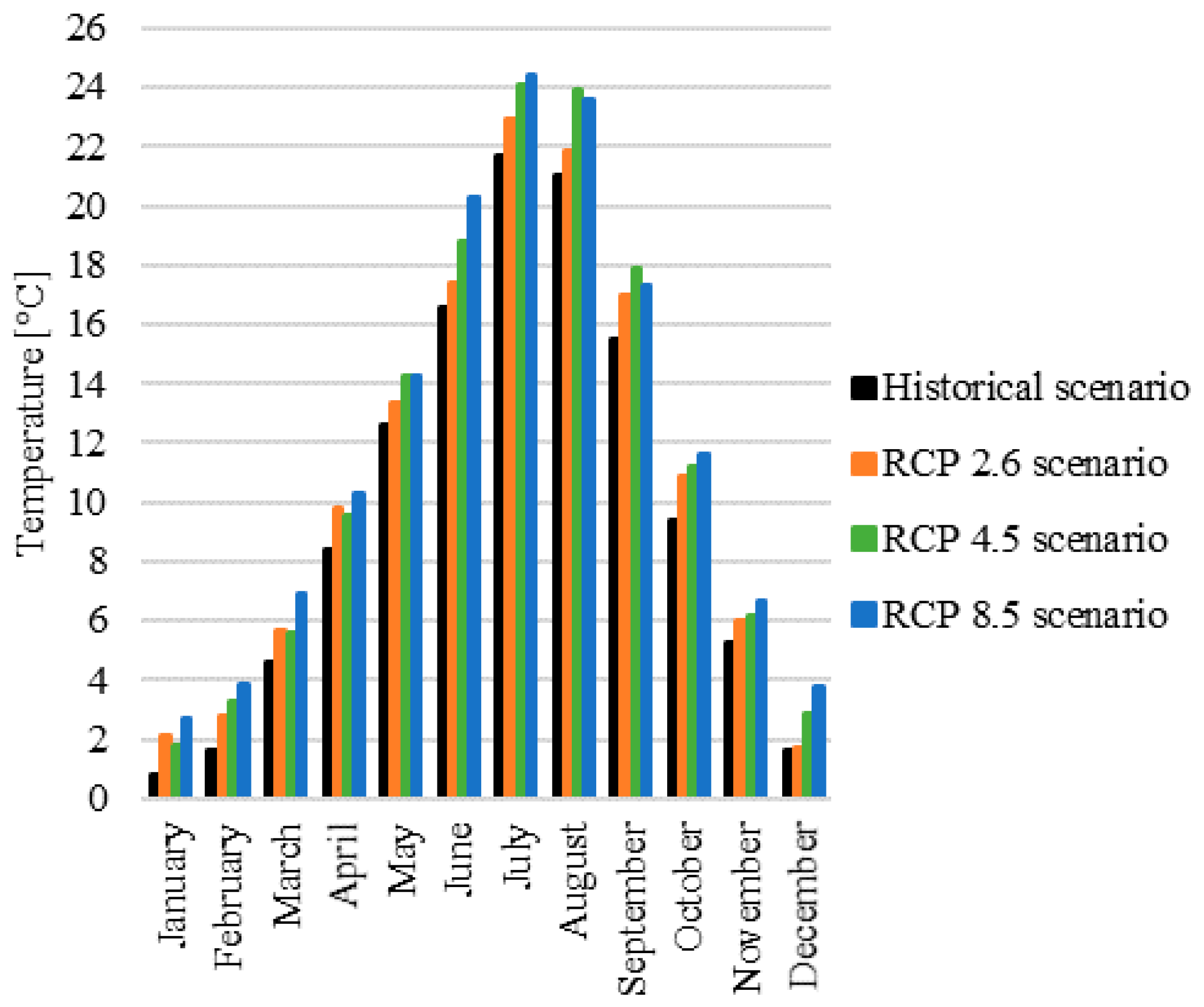
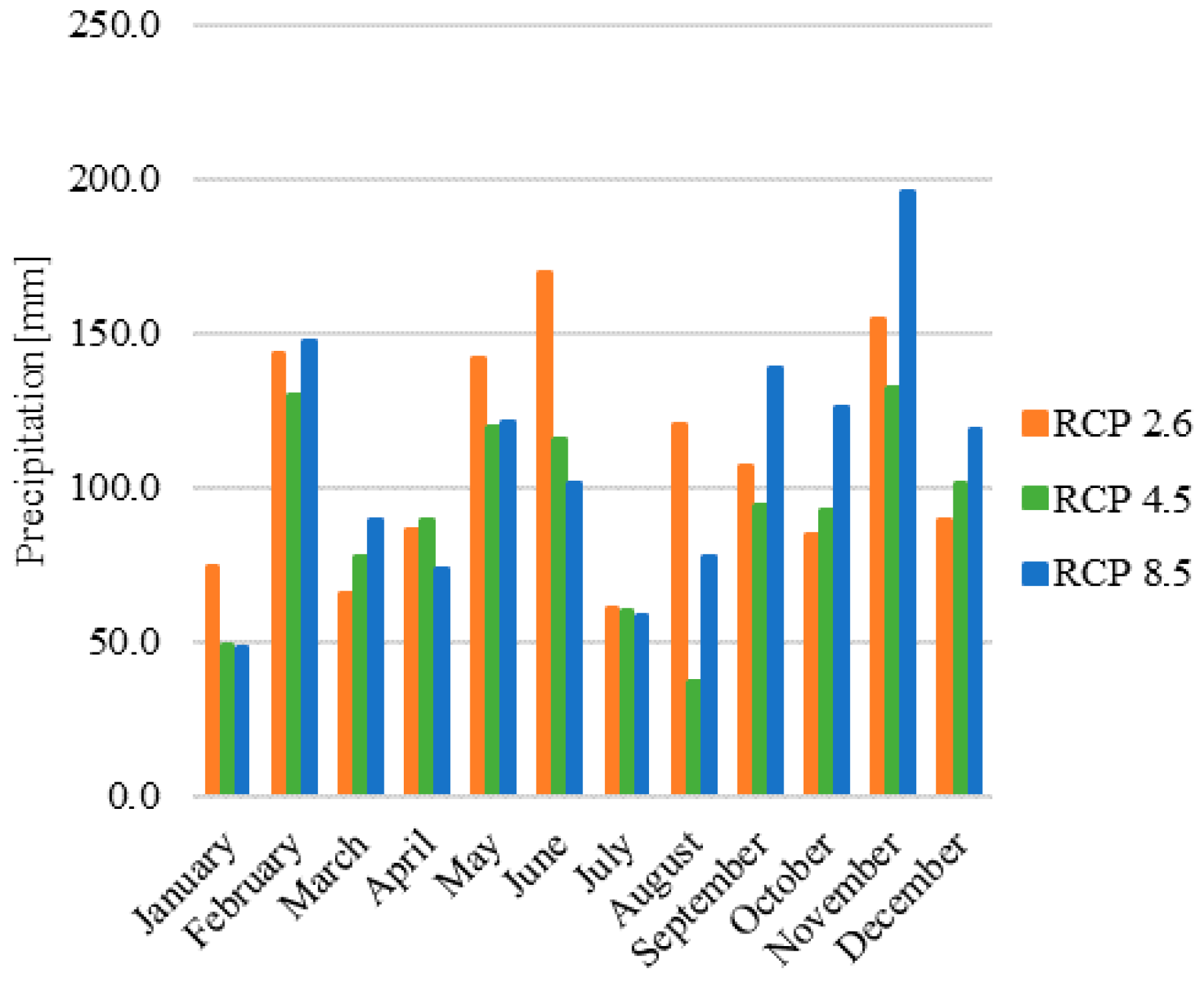
2.3. Climate Change Scenarios

Climate change scenarios at the basin scale were built on the basis of CORDEX data, which include time series of values of different parameters (precipitation, temperature, etc.) at specific grid points [22]. The following options were considered for this study:

• Driving model or Global Climate Model (GCM): a GCM can provide projections of how the earth’s climate may change in the future, on grid cells of around 1000 by 1000 km, and it is based on mathematical descriptions of the governing physical processes of the climate system. A GCM cannot supply an accurate representation of localized extreme events, but it drives the Regional Climate Model (RCM), incorporating the input domain for an RCM [23]. In this analysis, the selected GCM was the ICHEC-EC-EARTH [40].
• Regional Climate Model (RCM): The Regional Climate Model (RCM) is driven by the GCM; it can provide information on much higher spatial resolution because it is applied over a limited area. CORDEX data were calculated using RCM together with the dynamical downscaling technique [22,41]. In this work, the selected RCM was RCA4 (the surface processes of the Rossby Centre regional atmospheric climate model), described by the report of [42].
• Domain: a domain is a region where the regional downscaling takes place, and there are 14 different CORDEX domains. The European domain (EURO) covers the whole European continent. In this work, the domain used was EUR-11i, which has a resolution of 0.125 degrees, both in latitude and in longitude [41].

On the basis of the selection described above, three different climate scenarios (or climate projections) were considered for the middle of the century, according to the Representative Concentration Pathways (RCP) set by IPCC [2]: RCP 2.6 (from 2041 to 2060), RCP 4.5 (from 2041 to 2060), and RCP 8.5 (from 2041 to 2060). These scenarios are the representations of various possible future states of the climate system, based on both numerical model simulations that describe the complex processes and interactions affecting the climate system and information about anthropogenic climate forcing (socio-economic, technological, demographic factors and environmental development). The factors of anthropogenic activity are characterized in climate models as equivalent changes in greenhouse gas concentrations. Therefore, RCP scenarios in the EURO-CORDEX ensemble define pathways of the additional radiative forcing (in W/m²) caused by anthropogenic activity until the end of the 21st century (the value in 1750 is considered as a reference). RCP 8.5 represents very high greenhouse gas emission radiative forcing (8.5 W/m²), which continues to rise even after 2100. RCP 4.5 (radiative forcing value of 4.5 W/m²) is a stabilization scenario, because forcing will stabilize at their given value around the end of the century. RCP 2.6 (radiative forcing value of 2.6 W/m²) represents an aggressive mitigation scenario with a considerable negative future emission [23]. Finally, another stabilization scenario (RCP 6.0 with radiative forcing value of 6.0 W/m²) does exist, but it was not considered in this study because it is very similar to RCP 4.5.

In this research, the historical scenario (from 1986 to 2005) in the CORDEX dataset was also considered. The historical simulation had to be investigated, since this type of experiment is not synchronized with the observed climate.

By comparing historical and future simulations, relative values of future precipitation and temperature can be used to build future local climate scenarios starting from observed data (from 2008 to 2011 at Sarnico).

2.4. The Impact of Climate Change: Application of RUSLE Model

Monthly precipitation from 2041 to 2060 (considering different climate scenarios) is provided for each point of the grid used in the modeling chain selected for the study. Figure 3 shows as yellow dots the “RCM grid points”. The green arrow indicates point A, which is the relevant point belonging to the Guerna watershed in the grid: precipitation data for different climate change scenarios, corresponding to this point, were considered to evaluate climate change effects.

By comparing monthly precipitation historical simulations and future projections (RCP 2.6, RCP 4.5, RCP 8.5) shown in Figure 4, a correction factor (J) was derived for each month of the year, which was then applied to the observed precipitation in order to account for the expected change semi-hourly. Precipitation observations were provided by “Consorzio dell’Oglio” [25]; they were used in [21] and they are also described in Section 2.1. The correction factor in

Table 3. Monthly correction factor for precipitation and erosivity index in Sarnico.

Ji-month Coefficient [–]				Erosivity Index Re [MJ·mm·h−1·ha−1]
Month	RCP 2.6 Scenario	RCP 4.5 Scenario	RCP 8.5 Scenario	Current Climate	RCP 2.6 Scenario	RCP 4.5 Scenario	RCP 8.5 Scenario
January	1.29	0.85	0.83	20.6	36	14.7	13.9
February	1.59	1.44	1.64	43.9	123.4	98.1	131
March	0.95	1.12	1.29	31.3	28	39.9	55.3
April	0.96	0.99	0.81	86.1	78.1	84.8	54.9
May	1.37	1.16	1.18	177.7	373.9	249.9	261.2
June	1.23	0.84	0.74	312.3	510.8	209.1	153.8
July	0.74	0.73	0.72	457.1	223.7	220.9	207.5
August	1.12	0.34	0.72	394.2	510.9	33.2	181.9
September	0.85	0.76	1.11	468.9	323	243.1	597.8
October	0.82	0.90	1.23	98.1	63.2	77.4	157
November	0.92	0.79	1.17	189.1	155.8	138.7	271.9
December	0.78	0.88	1.03	56.8	33	43.1	61

was determined by the following equation:

$${\mathrm{J}}_{\mathrm{i}-\mathrm{month}}=\frac{{\left({\mathrm{h}}_{\mathrm{future}\_\mathrm{scenario}}\right)}_{\mathrm{i}-\mathrm{month}}}{{\left({\mathrm{h}}_{\mathrm{historical}\_\mathrm{scenario}}\right)}_{\mathrm{i}-\mathrm{month}}}$$

(6)

where ${\left({\mathrm{h}}_{\mathrm{future}\_\mathrm{scenario}}\right)}_{\mathrm{i}-\mathrm{month}}$ and ${\left({\mathrm{h}}_{\mathrm{historical}\_\mathrm{scenario}}\right)}_{\mathrm{i}-\mathrm{month}}$ are the mean monthly precipitation values shown in Figure 4 for different scenarios.

The multiplicative coefficient J_i-month was applied to the observed half an hour rainfall data from 2008 to 2011 to project the 4-year-long time series into the future.

Then, a new value for the R factor was computed with the modified precipitation time series. According to analyzed CORDEX outputs, yearly precipitation is reduced for RCP 4.5. Moreover, the multiplication coefficients concerning the months with highest erosivity index (June, July, August, and September) are much lower than 1 for RCP 4.5 (see Table 3); they are lower than 1 (on average) also for RCP 8.5, while their value is lower than 1 only for July and September for RCP 2.6. The R factor value set in [21] was 2336 MJ∙mm∙ha⁻¹∙h⁻¹∙year⁻¹.

The other factors (K factor, LS factor, C factor, and P factor) required for the implementation of the RUSLE model, as described in Paragraph 2.2, were not modified with respect to values set in [21]. Therefore, the K value was 0.038 t∙ha∙h∙ha⁻¹∙MJ⁻¹∙mm⁻¹, and the maximum, minimum, and mean values of LS factor were respectively 41.78, 0.027, and 14.09. C and P factor values were as follows (

Table 4. C factor values and P factor values. C: cover-management factor, P: supporting practices factor.

Land Use	C Factor	P Factor
Wooded, reforested and forested area	0.002	1
Grassland	0.07	1
Agricultural area	0.45	1
Orchard and vineyard	0.37	0.45
Urban area	0.003	1
Bare areas	0.36	1

).

2.5. The Impact of Climate Change: Application of EPM Model

In this model, both precipitation and temperature information are relevant: monthly precipitation and monthly air temperature from 2041 to 2060 (considering different climate scenarios) can be extracted from the CORDEX dataset for each point of the RCM grid. As for the RUSLE method, precipitation data for different climate change scenarios were considered only for the grid point inside the boundaries of the basin. Temperature data corresponding to grid point B (indicated by the orange arrow in Figure 3) were useful to estimate the temperature coefficient (T) for the future climate, as it is further explained.

Just as in the case of the RUSLE model application (Section 2.4), the multiplicative J_i-month coefficient was applied to the same observed climate data (from 2008 to 2011) that are described in Section 2.1 and that were also reported and used in [21] to estimate the mean annual amount of precipitation (H). These data were used to evaluate the precipitation regime in order to build local climate change scenarios.

The temperature coefficient (T) was calculated by applying Equation (3), taking into account its spatial variability, as reported in [21] for the actual climate. Sarnico temperature values are also described in Section 2.1. A linear decrease of temperature as a function of altitude was assumed.

Using monthly temperature data from 2041 to 2061 (for RCP 2.6, RCP 4.5, and RCP 8.5 scenarios) and from 1986 to 2005 (for the historical scenario) referring to point A (h_A = 433.8 m a.s.l. in the CORDEX database experiment) (see Figure 3 and Figure 5) monthly temperature difference $\overline{\Delta \mathrm{t}}$ were computed (

Table 5. Monthly temperature difference between future and historical scenarios.

Month	Temperature Difference $\overline{\mathsf{\Delta }\mathbf{t}}$ [°C] at Point A
	RCP 2.6 Scenario	RCP 4.5 Scenario	RCP 8.5 Scenario
January	1.36	1.00	1.91
February	1.16	1.62	2.30
March	1.13	1.07	2.37
April	1.43	1.20	1.90
May	0.78	1.70	1.72
June	0.84	2.22	3.71
July	1.22	2.48	2.71
August	0.97	2.99	2.61
September	1.48	2.37	1.79
October	1.49	1.74	2.15
November	0.65	0.91	1.38
December	0.19	1.32	2.24

):

$${\overline{\Delta \mathrm{t}}}_{\mathrm{i}-\mathrm{month}}={\left({\overline{\mathrm{t}}}_{\mathrm{i}-\mathrm{month}}\right)}_{\mathrm{RCP} \mathrm{scenario}}-{\left({\overline{\mathrm{t}}}_{\mathrm{i}-\mathrm{month}}\right)}_{\mathrm{historical} \mathrm{scenario}}.$$

(7)

Then, the slope of the regression line (vs. elevation), for each month and considering each RCP future scenario, was computed:

$${\overline{\mathrm{Slope}}}_{\mathrm{i}-\mathrm{month}}=\frac{{\left({\overline{\mathrm{t}}}_{\mathrm{A}}\right)}_{\mathrm{i}-\mathrm{month}}-{\left({\overline{\mathrm{t}}}_{\mathrm{B}}\right)}_{\mathrm{i}-\mathrm{month}}}{\left({\mathrm{h}}_{\mathrm{A}}\right)-\left({\mathrm{h}}_{\mathrm{B}}\right)}$$

(8)

where $\overline{\mathrm{t}}$ is the mean monthly temperature at grid point A and at point B.

The grid point B location is indicated in Figure 3 (h_B = 796.6 m a.s.l. in the CORDEX database). The mean monthly temperatures at point A (${\overline{\mathrm{t}}}_{\mathrm{A}}$) and at point B (${\overline{\mathrm{t}}}_{\mathrm{B}}$), provided by the CORDEX experiment, are shown respectively in Figure 5 and Figure 6.

Since the elevation of point A is known, Equation (9) can finally be used to find the monthly temperature t in the current climate at that point:

$${\left({\mathrm{t}}_{ \mathrm{A}}\right)}_{\mathrm{i}-\mathrm{month}}=({\mathrm{Slope}}_{\mathrm{i}-\mathrm{month}})\left({\mathrm{h}}_{\mathrm{A}}-{\mathrm{h}}_{\mathrm{Sarn}.}\right)+{\left({\mathrm{t}}_{\mathrm{Sarn}.}\right)}_{\mathrm{i}-\mathrm{month}}.$$

(9)

${\mathrm{Slope}}_{\mathrm{i}-\mathrm{month}}$ is the slope of the straight line equation for each month, using temperature data from 2008 to 2011 provided by ARPA LOMBARDIA [26] at Sarnico station and at Ranzanico station, similarly to [21]. The results are shown in Figure 7.

Information obtained from previous steps (the temperature difference $\overline{\Delta \mathrm{t}}$, the slope of the straight line equation for each month ${\overline{\mathrm{Slope}}}_{\mathrm{i}-\mathrm{month}}$, and the monthly observed temperature t at point A) were used to create a monthly temperature map (t_{MAP_CC})_i-month with a spatial variability for each month and for each RCP scenario, according to the following equation:

$${\left({\mathrm{t}}_{\mathrm{MAP}\_\mathrm{CC}}\right)}_{\mathrm{i}-\mathrm{month}}=({\overline{\mathrm{Slope}}}_{\mathrm{i}-\mathrm{month}})\left(\mathrm{DEM}-{\mathrm{h}}_{\mathrm{A}}\right)+{\left({\mathrm{t}}_{\mathrm{A}}+\overline{\Delta \mathrm{t}}\right)}_{\mathrm{i}-\mathrm{month}}$$

(10)

where DEM is the Digital Elevation Model, whose spatial resolution is 5 m × 5 m. The DEM map of the Guerna catchment is reported in [21], and Table 1 contains its maximum and minimum value. This map shows the higher and lower altitude values respectively in the northern and in the southern part of the study area.

The 12 monthly temperature maps were used to create a mean annual temperature map (t_{MAP_CC})_{mean anuual} (with a spatial variability and considering each scenario of climate change) solving the following equation:

$${\left({\mathrm{t}}_{\mathrm{MAP}\_\mathrm{CC}}\right)}_{\mathrm{mean} \mathrm{annual}}=\frac{1}{12}{{\displaystyle \sum }}_{\mathrm{i}=1}^{12}{\left({\mathrm{t}}_{\mathrm{MAP}\_\mathrm{CC}}\right)}_{\mathrm{i}-\mathrm{month}}.$$

(11)

The mean annual temperature map (t_{MAP_CC})_{mean annual} was finally used to solve Equation (3) in a GIS environment.

It should be recorded that the H value set in [21] without considering climate change scenarios was 1250.55 mm/year and the maximum, minimum, and the mean value of the T coefficient (taking into account its spatial variation in the study area) set in [21], without considering climate change scenarios was respectively 1.22, 1.01, and 1.14.

The value of the coefficient of erosion (Z) was not changed with respect to the value reported in [21].

Table 6. Coefficient values.

Coefficient	Maximum Value	Minimum Value	Mean Value
${\mathrm{X}}_{\mathrm{a}}$ (land use coefficient)	0.90	0.13	0.29
$\mathrm{Y}$ (coefficient of soil resistance to erosion)	2.00	0.90	1.22
$\mathsf{\phi }$ (coefficient value for the observed erosion processes)	0.90	0.15	0.30
Z (coefficient of erosion)	2.96	0.00	0.33

shows the maximum, minimum and mean value of the Z coefficient and of the coefficients used in Equation (4) to estimate it. These coefficient values were obtained by maps reported [21].

As shown in Table 1 and in the land use map in [21], most of the catchment area is occupied by wooded forests, to which ${\mathrm{X}}_{\mathrm{a}}$ = 0.125 was assigned. As described in Section 2.1 and reported in [21], the lithological map reveals the presence of limestone in most of the territory, to which $\mathrm{Y}$ = 1.20 was assigned. The hydrogeological instability map described in Section 2.1 and reported in [21] shows that most of the area of the catchment is without visible erosion effects; to this area, $\mathsf{\phi }$ = 0.15 was attributed.

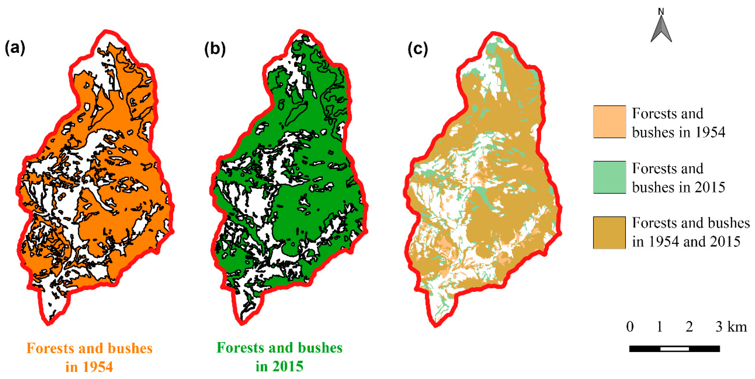
2.6. The Effect of Climate Change on Land Use

The paragraphs above describe how to compute soil loss also considering the effects of climate change, by solving Equations (1) and (2) respectively for the RUSLE and EPM method. As regards the RUSLE method, the computed soil loss (A) was calculated by changing only the rainfall erosivity factor (R factor) according to climate change. On the other hand, considering the EPM equation, the average annual production of erosional sediment (W_g) was estimated by changing both the mean annual amount of precipitation (H) and the temperature coefficient (T), considering the impact of climate change. Therefore, in both cases, the future variations of the cover management factor were omitted.

Nevertheless, the land use over time in the Guerna catchment was analyzed in order to understand the changes that have taken place over the past years. This operation was implemented by the comparison between the land use map in 1954 and the land use map in 2015; both maps were made available by “Geoportale della Lombardia” [24].

The analysis established that most of the Guerna catchment area is covered by forest (broadleaved forests, coniferous forests, mixed forests dominated by coppice formations, riparian forests) and bushes (with the significative presence of high and arboreal shrub species), both in 1954 and in 2015 (Figure 8). In particular, the most recurrent type of tree that remains in the forest in time is the broadleaved tree.

Finally, the analysis of precipitation and temperature in the past in the study area was performed in order to relate the detected change in land use to the monitored climate changes. The variability of these parameters is the most important element that can affect land cover, in particular its vegetation. The annual precipitation trend (from 1960 to 2016 [25,26]) and temperature trend (from 1973 to 2016 [26,43]) available at Sarnico were investigated. It was found that there was not a large variability of these climatic parameters over the years, in comparison with climate change scenarios.

For these reasons and to remain in security, in the study area, the impact of climate change on land use was neglected.

3. Results

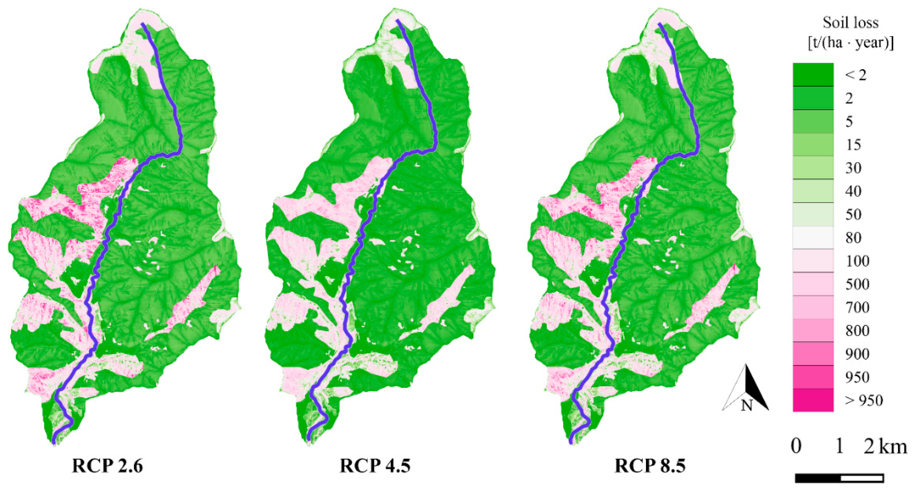
3.1. The Impact of Climate Change According to the RUSLE Model

Projected rainfall data obtained in accordance with the procedure described in Section 2.4 were used in order to estimate a new R factor value for each scenario:

• RCP 2.6 scenario: R factor = 2460 MJ·mm/(ha·h·year)
• RCP 4.5 scenario: R factor = 1453 MJ·mm/(ha·h·year)
• RCP 8.5 scenario: R factor = 2147 MJ·mm/(ha·h·year)

The computed soil loss A was calculated by solving Equation (1) and considering the three different future scenarios (Figure 9). The mean value (A_{_mean}) and the total value (A_{_tot}) in the Guerna catchment of computed soil loss in future scenarios are shown in

Table 7. Computed soil loss (Revised Universal Soil Loss Equation (RUSLE) method) considering different future scenarios.

Future Scenario	A_mean [t/(ha∙Year)]	A_tot [t/(Year)]
RCP 2.6	91.7	283,427.5
RCP 4.5	54.2	167,406.6
RCP 8.5	80.0	247,365.4

.

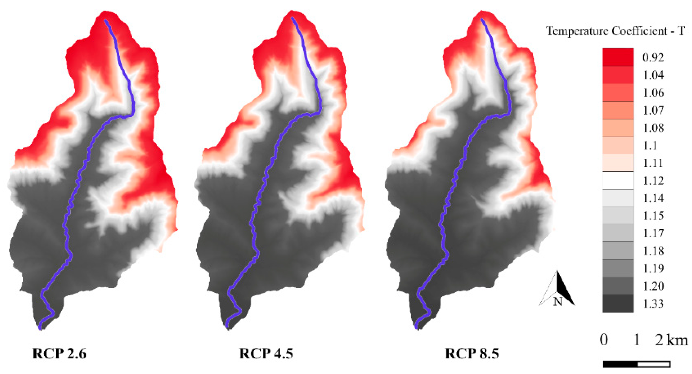
3.2. The Impact of Climate Change According to the EPM Model

Projected rainfall data, derived in accordance with the procedure described in Section 2.5, were used in order to estimate a new mean annual amount of precipitation (H) for each scenario. The results are shown below and in Figure 10 (reporting monthly mean values):

• RCP 2.6 scenario: H = 1300.2 mm/(year)
• RCP 4.5 scenario: H = 1101.1 mm/(year)
• RCP 8.5 scenario: H = 1299.6 mm/(year).

The mean annual temperature map (t_{MAP_CC})_{mean annual} was determined, in accordance with the procedure described in Section 2.5, by considering each of the future scenarios (RCP 2.6, RCP 4.5, and RCP 8.5). These maps were used in order to solve Equation (3) and create the maps of the temperature coefficient (T) shown in Figure 11.

The mean value in the Guerna catchment of the temperature coefficient (T) for the future scenarios are the following:

• RCP 2.6 scenario: T = 1.15
• RCP 4.5 scenario: T = 1.18
• RCP 8.5 scenario: T = 1.21.

The map of the average annual production of erosional sediment W_g was calculated by solving Equations (2) and (5), considering the three different future scenarios (Figure 12). In Equation (5), A is the DEM cell area (A = 0.000025 km²).

The mean value (W_{g_mean}) and the total value (W_{g_tot}) in the Guerna catchment of computed soil loss in future scenarios are shown in

Table 8. Production of erosional sediment (EPM model) considering different future scenarios.

Future Scenario	Wg_mean [m3/(Cell∙Year)]	Wg_tot [m3/(Year)]
RCP 2.6	0.029	36,358.0
RCP 4.5	0.025	31,516.0
RCP 8.5	0.030	37,881.5

.

3.3. Comparison with the Scenario without Climate Change

Table 9. Summary of the results.

Method	Without Considering Climate Change Scenario	Climate Change Scenario
		RCP 2.6	RCP 4.5	RCP 8.5
RUSLE [t/year]	269,141	283,428	167,407	247,365
EPM [m3/year]	34,193	36,358	31,516	37,882

summarizes the results obtained for the current and the future climate.

Table 10. Results of the statistical trend of the data in the Guerna catchment, considering different scenarios and using the RUSLE model.

Scenario	RUSLE Results (A) [t/(ha∙Year)]
	Maximum Value	Mean	Standard Deviation
Without climate change	1706.9	87.1	203.3
RCP 2.6	1797.5	91.7	214.1
RCP 4.5	1061.7	54.2	126.4
RCP 8.5	1568.8	80.0	186.8

and

Table 11. Results of the statistical trend of the data in the Guerna catchment, considering different scenarios and using the EPM model.

Scenario	EPM Results (Wg) [m3/(Cell∙Year)]
	Maximum Value	Mean	Standard Deviation
Without climate change	0.606	0.028	0.040
RCP 2.6	0.664	0.029	0.043
RCP 4.5	0.574	0.025	0.037
RCP 8.5	0.686	0.031	0.045

list the results achieved by the statistical treatment of the data obtained for different climate change scenarios (also represented in Figure 9 and Figure 12) and including the scenario without climate change.

By considering an average specific weight of 2.65 t/m³ [44], soil loss computed by the RUSLE equation for the Guerna watershed is between two and three times higher than its evaluation according to the EPM method both in the current and in the future scenarios, as shown in

Table 12. Summary of the results considering a specific weight of 2.65 t/m³.

Method	Without Considering Climate Change Scenario	Climate Change Scenario
		RCP 2.6	RCP 4.5	RCP 8.5
RUSLE [t/year]	269,141	283,428	167,407	247,365
EPM [t/year]	90,612	96,349	83,517	100,386

.

4. Discussions

Ref [19] conducted a study to estimate actual erosion over the whole alpine space and a spatial analysis of soil erosion trends in different IPCC scenarios. The main objective was the assessment of soil erosion in relation to climate change. The RUSLE equation was applied to the whole alpine space and it produced, with a spatial resolution of 100 m, the map of actual soil erosion and the maps defining soil erosion rates in IPCC A2 and B2 scenarios 2070–2100. From a comparison between actual and soil losses in A2 and B2 scenarios, it came out that the model did not present relevant rises in erosion rates [19]. In addition, considering the application of the RUSLE equation in the Guerna watershed and the three climate change scenarios, the model did not report relevant increases. In particular, the RCP 2.6 and RCP 8.5 scenarios show respectively a low growth and a low reduction of entity of soil losses, while the RCP 4.5 scenario shows a strong reduction in soil loss (Table 9).

Ref [45] investigated the future climate change scenarios of soil erosion in Val Camonica and Lake Iseo, which is one valley of the Italian Alps extending for about 1800 km², and it is adjacent to the Guerna catchment. In this case study, simulations were done with the D-RUSLE (Dynamic Revised Universal Soil Loss Equation) model [46,47], which, in comparison with the RUSLE model, accounts also for snow cover and land cover dynamics. The results of this study show that the mean annual erosion rate in future scenarios can increase or decrease, and this fact depends on climatic parameters (precipitation and temperature). Generally, rainfall amount and intensities usually increase the erosion rate. These elements are consistent with the findings of our study area.

Refs [45,48] analyzed the RCM’s projection for the Alpine region at the end of the 21st century, and they found that the projected temperature always increases, but the annual precipitation trend is variable because it can increase or decrease; in particular, the expected changes are an increase in winter precipitation and a decrease in summer precipitation. These trends are confirmed also considering the climate change scenarios analyzed in our work (Table 3 and Table 5).

Moreover, as [45] also claims, it must be pointed out that although rainfall amounts and intensities usually increase the erosion rate, it is rather difficult to compare our results with existing literature because different studies have substantial differences (for example, working scale, topographic and land use features, the models used both to estimate soil erosion and to project climate changes).

Considering the Guerna catchment, the mean amount of precipitation H for the RCP 2.6 and RCP 8.5 scenarios is higher than the H value estimated without considering climate change, but it is lower than that for the RCP 4.5 scenario (see [21] and Section 3.2). This result is in line with the prediction of IPCC [2], according to which precipitation patterns can either rise or reduce in the future climate. The soil loss calculated using the EPM method for the RCP 2.6 and RCP 8.5 scenarios is larger than the value estimated without considering climate change, but it is smaller for the RCP 4.5 scenario (Table 9). Indeed, soil erosion is likely to increase with the increased rainfall amount. However, applying the RUSLE equation, the computed soil loss is higher than the value estimated without considering climate change only for the RCP 2.6 scenario (Table 9). The reason for this result can be found in the R factor value, which is larger than the value estimated without considering climate change only for the RCP 2.6 scenario (see [21] and Section 3.1). Indeed, the R factor also takes into account the kinetic energy in a single rainfall event and the rainfall intensity that affects soil loss greatly. Ref [49] demonstrated, through experiments using a rainfall simulator, the importance of rainfall kinetic energy for a better understanding of erosion processes.

Temperature is predicted to rise in all future scenarios considered in the Guerna watershed (see [21] and Section 3.2). This is in accordance with other case studies (in North America, Asia and Europe), which are summarized in [1], and the undisputable global warming trend [2], as a consequence of higher CO₂ emissions that are related to anthropogenic or socio-economic factors [1]. When atmospheric CO₂ concentration increases, as it happens in the future climate scenarios analyzed, the temperature also increases, and it leads to changes, for example in soil moisture, evapotranspiration rates, infiltration capacity of the soil, and runoff. For these reasons, soil erosion is affected indirectly by raising the temperature [1,50].

Concerning the effect of climate change on land use, the future variations of the cover management factor were neglected because of the evolution of land use over time and the results of the analysis on precipitation and temperature trends. In fact, as regards the evolution of land cover over the years, Figure 8 shows that the areas occupied by forests and bushes are very similar in 1954 and in 2015. In fact, the green areas (“Forests and bushes in year 2015”) in Figure 8c are the areas covered by forests and bushes only in 2015. From the analysis of the land use map (“Uso del suolo storico (1954)”), it emerged that in 1954, those areas were primarily occupied by grasslands and by sparse vegetation arable lands, vineyards, and chestnut trees. The orange areas (“Forests and bushes in 1954”) in Figure 8c are the areas covered by forests and bushes only in 1954. From the analysis of the land use map (DUSAF 5.0—“Uso del suolo 2015”), it was found that in 2015, those areas were occupied by farms, residential areas, industrial establishments, road networks, and sport facilities and by a minor part of grasslands, vineyards, olive trees, and arable lands. The green areas and the orange areas in Figure 8c cover respectively about 3.4 and 1.5 km². Thereby, it can be stated that there was an increase of around 1.9 km² of forests and bushes in 2015, compared with 1954. The brown areas (“Forests and bushes in 1954 and in 2015”) in Figure 8c that cover most of the Guerna catchment show the places covered by forests and bushes both in 1954 and in 2015. Therefore, in the Guerna watershed, the land use map analysis showed an approximate 6% increase in forests in the last decades, further protecting the soil from water erosion. As resulting from the C factor values and land use coefficient (X_a) values respectively in the RUSLE and EPM equations reported in [21] and described in Section 2.4 and Section 2.5, the presence of forests and bushes that cover most of the study area (see Figure 8) mitigates water erosion more than grasslands, agricultural areas, orchards, and vineyards. The water erosion in urban areas (residential areas, industrial establishments, road networks, etc.) is very low, as is the value of the C factor in the RUSLE model. However, orchards and vineyards can reduce water erosion also because of their P factor value (see P factor values in [21] and in Section 2.4). Ref [51] analyzed the spatial variability of erosion rates in the small watersheds of the Three-Gorge Reservoir drainage area in China. Taking also into consideration the land use map, they found that the areas of crop land are characterized by higher erosion rates while wooded areas present very low erosion rates. Ref [19] conducted a study to estimate the actual erosion using the RUSLE method over the whole alpine space. They analyzed soil erosion trends in IPCC A2 and B2 scenarios [18]. Even in this study, the factors K, LS, and C coincided with the ones used for erosion estimation that does not consider climate change (actual erosion estimation). In that regard, they claimed, first, that soil erosion trends in the alpine region are primarily due to changes in rainfall patters. However, they argued that a better estimation of soil losses in climate change scenarios could be achieved by considering future variations of the cover management factor [19]. The Guerna basin is located in an alpine region and then, in accordance with [19], only the rainfall and temperature regime were considered to evaluate the effects of climate change on water erosion.

Finally, in order to better justify the use of the same cover management factor in future scenarios, the analysis of observed precipitation and temperature trends over the years in the study area was performed using available data as described in Section 2.6. The analysis showed that precipitation is an annual changeable parameter, above and below its mean value (1089 mm), from 1960 to 2016 at Sarnico station; its maximum and minimum registered values are respectively 1745 and 628 mm. This trend is very similar to the trend of the future scenarios that were considered on the basis of CORDEX data, and the observed variability over the years does not exceed the variability of the future scenarios, where the largest difference between the maximum and the minimum value of precipitation is 985 mm. Concerning temperature, the analysis of observed data at Sarnico over the years showed a gradual increase. The minimum and the maximum annual values were registered respectively in the past (11.4 °C) and in recent years (14.9 °C); the mean annual measured value over the years is 13.1 °C. In addition, future scenarios on the basis of CORDEX data reveal an increasing of temperature (see Table 5), and the value of the annual temperature difference is not meaningful compared to the difference of the observed temperature.

These considerations lead to the conclusion that, considering the effects of climate changes, the future variations of the cover management factor in the Guerna watershed can be omitted. Indeed, in the last 60 years, there have not been significant transformations in land use, except for a small increase in forests and bushes that slightly reduced water erosion. In addition, it was found that there was not a large variability of precipitation and temperature over the years, in comparison with climate change scenarios. Therefore, keeping the same cover management factor in future scenarios improves security, since the introduced approximation is expected to eventually overestimate water erosion.

5. Conclusions

The general aim of this research was to analyze soil erosion trends in a small alpine basin, considering different IPCC (Intergovernmental Panel on Climate Change) future scenarios: RCP 2.6, RCP 4.5, and RCP 8.5.

In this research, the RUSLE [14] and the EPM [15] empirical methods were used to analyze soil erosion and estimate soil loss for the Guerna catchment, a small mountain basin located in Northern Italy. The most important climate variables in these models are precipitation and air temperature. The EPM method accounts for a more complete description of the meteorological forcing, since both precipitation and air temperature are included in the equation, while the RUSLE method accounts for climatic features only through precipitation but considers also the effect of soil particle size distribution.

Concerning the RUSLE model, the rainfall erosivity factor (R factor) was modified to consider the effects of climate change in line with IPCC scenarios. The other factors (K factor, LS factor, C factor, and P factor) requested for the implementation of the RUSLE model had no changes, compared to the case without climate change reported in [21].

Concerning the EPM method, the mean annual amount of precipitation (H) and the temperature coefficient (T) were modified in order to assess the impact of climate in accordance with IPCC scenarios. The coefficient of erosion (Z) has not undergone any modifications compared with the scenario without climate change described in [21].

In accordance to [19] and with the analysis of land use evolution shown in Section 2.6 and Section 3.3, only rainfall and temperature regime were considered to evaluate the effects of climate change on water erosion; the future variations of the cover management factor were omitted, improving security. Moreover, in order to better justify the use of the same cover management factor in future scenarios, the analysis of observed precipitation and temperature trend in the past was performed, and it was found that there was not a large variability of precipitation and temperature over the years, in comparison with climate change scenarios on the basis of CORDEX data.

The results showed that the climate change impacts on water erosion may not be negligible even by the middle of this century. According to the EPM method and RCP 2.6, RCP 4.5, and RCP 8.5, the annual average soil loss could change by 6–10% on a basin scale. It was also emphasized that soil erosion rates may increase or decrease under climate change, depending on a combination of different elements. The seasonality in peak rainfall intensity is finally playing a major role. Indeed, in the Guerna catchment, the soil loss calculated using the EPM method for RCP 2.6 and RCP 8.5 scenarios is larger than the value estimated without considering climate change, but it is smaller for the RCP 4.5 scenario, because soil erosion is likely to increase with the increased rainfall amount that occurs only considering the RCP 2.6 and RCP 8.5 scenarios. The EPM method does not take into account rainfall intensity in a single rainfall event. By applying the RUSLE equation, the computed soil loss is higher than the value estimated without considering climate change only for the RCP 2.6 scenario, and the reason for this result is the R factor value, which takes into account the rainfall intensity in a single rainfall event.

Concerning temperature, only the EPM model considers this parameter that is predicted to rise in all future scenarios.

Empirical models still provide a useful analysis tool when detailed information is missing. Nevertheless, field measurements and the knowledge of the future land use variations in the study area could further increase the accuracy and reliability of the whole methodology. Despite current limitations, this study complements the existing literature on the effects of climate change on soil erosion.

References

1. Li, Z.; Fang, H. Impacts of climate change on water erosion: A review. Earth Sci. Rev. 2016, 163, 94–117. [Google Scholar] [CrossRef]
2. Stocker, T.F.; Qin, D.; Plattner, G.; Tignor, M.M.B.; Allen, S.K.; Boschung, J.; Nauels, A.; Xia, Y.; Bex, V.; Midgley, P.M. IPCC 2013. In Climate Change 2013: The Physical Science Basis. Contribution of Working Group I to the Fifth Assessment Report of the Intergovernamental Panel on Climate Change; Cambridge University Press: Cambridge, UK; New York, NY, USA, 2013; 1585p. [Google Scholar]
3. Prusky, F.F.; Nearing, M.A. Runoff and soil-loss responses to changes in precipitation: A computer simulation study. J. Soil Water Conserv. 2002, 57, 7–16. [Google Scholar]
4. Routschek, A.; Schmidt, J.; Kreienkamp, F. Impact of climate change on soil erosion – a high resolution projection on catchment scale until 2100 in Saxony/Germany. Catena 2014, 121, 99–109. [Google Scholar] [CrossRef]
5. Nearing, M.A.; Jetten, V.; Baffaut, C.; Cerdan, O.; Couturier, A.; Hernandez, M.; Le Bissonnais, Y.; Nichols, M.H.; Nunes, J.P.; Renschler, C.S.; et al. Modeling response of soil erosion and runoff to changes in precipitation and cover. Catena 2005, 61, 131–154. [Google Scholar] [CrossRef]
6. Nearing, M.A.; Prusky, F.F.; O’Neal, M.R. Expected climate change impacts on soil erosion rates: A review. J. Soil Water Conserv. 2004, 59, 43–50. [Google Scholar]
7. Le Van, T.; Ranzi, R.; Rulli, M.C. Modeling Soil Erosion and Sediment Load for Red River Basin (Vietnam): Impact of Land Use Change and Reservoirs Operation. In Proceedings of the 2018 IEEE International Conference on Environment and Electrical Engineering and 2018 IEEE Industrial and Commercial Power Systems Europe (EEEIC/I&CPS Europe), Palermo, Italy, 12–15 June 2018. [Google Scholar]
8. Ranzi, R.; Le, T.H.; Rulli, M.C. A RUSLE approach to model suspended sediment load in the Lo river (Vietnam): Effects of reservoirs and land use changes. J. Hydrol. 2012, 422–423, 17–29. [Google Scholar] [CrossRef]
9. Nunes, J.P.; Seixas, J.; Keizer, J.J. Modeling the response of within-storm runoff and erosion dynamics to climate change in two Mediterranean watershed: A multi-model, multi-scale approach to scenario design and analysis. Catena 2013, 102, 27–39. [Google Scholar] [CrossRef]
10. Ricci, G.F.; Jeong, J.; De Girolamo, A.M.; Gentile, F. Modelling management practices to reduce soil erosion in an agricultural watershed in Southern Europe. In Proceedings of the SWAT Conference, Brussels, Belgium, 17–21 September 2018. [Google Scholar]
11. Li, Z.; Liu, W.Z.; Zhang, X.C.; Zheng, F.L. Assessing the site-specific impacts of climate change on hydrology, soil erosion and crop yields in the Loess Plateau of China. Clim. Chang. 2011, 105, 223–242. [Google Scholar] [CrossRef]
12. Salazar, S.; Francés, F.; Komma, J.; Blume, T.; Francke, T.; Bronstert, A.; Blöschl, G. A comparative analysis of the effectiveness of flood management measures based on the concept of “retaining water in the landscape” in different European hydroclimatic regions. Nat. Hazard. Earth Sys. 2012, 12, 3287–3306. [Google Scholar] [CrossRef] [Green Version]
13. De Vente, J.; Poesen, J. Predicting soil erosion and sediment yield at the basin scale: Scale issues and semi-quantitative models. Earth Sci. Rev. 2015, 71, 95–125. [Google Scholar] [CrossRef]
14. Renard, K.G.; Foster, G.R.; Weesies, G.A.; Porter, J.P. RUSLE Revised universal soil loss equation. J. Soil Water Conserv. 1991, 46, 30–33. [Google Scholar]
15. Gavrilovic, Z. The use of an empirical method (Erosion Potential Method) for calculating sediment production and transportation in unstidied or torrential streams. In International Conference River Regime; Jhon Wiley & Sons: Chichester, UK, 1988; pp. 411–422. [Google Scholar]
16. Fowler, H.J.; Blenkinsop, S.; Tebaldi, C. Linking climate change modelling to impacts studies: Recent advances in downscaling techniques for hydrological modelling. Int. J. Climatol. 2007, 27, 1547–1578. [Google Scholar] [CrossRef]
17. Nakicenovic, N.; Swart, R. Special Report on Emissions Scenarios: A Special Report of Working Group III of the Intergovernmental Panel on Climate Change; Cambridge University Press: Cambridge, UK, 2000; ISBN 0-521-80493-0. [Google Scholar]
18. The Core Writing Team; Pachauri, R.K.; Reisinger, A. IPCC 2007: Climate Change 2007: Synthesis Report. Contribution of Working Groups I, II and III to the Fourth Assessment Report of the Intergovernmental Panel on Climate Change; IPCC: Geneva, Switzerland, 2007; p. 104. [Google Scholar]
19. Bosco, C.; Rusco, E.; Montanarella, L.; Oliveri, S. Soil erosion risk assessment in the alpine area according to the IPCC scenarios. In Threats to Soil Quality in Europe; Toth, G., Montanarella, L., Rusco, E., Eds.; Joint Research Centre in Ispra: Cadrezzate (VA), Italy, 2008; pp. 47–58. Available online: http://publications.jrc.ec.europa.eu/repository/handle/JRC46574 (accessed on 27 May 2020). [CrossRef]
20. Confortola, G.; Soncini, A.; Bocchiola, D. Climate change will affect hydrological regimes in the Alps. J. Alp. Res. Rev. de Géographie Alp. 2013, 101. [Google Scholar] [CrossRef] [Green Version]
21. Berteni, F. Sediment Yield and Transport: Estimation and Climate Influence. Ph.D. Thesis, University of Brescia, Brescia, Italy, 5 March 2019. [Google Scholar]
22. CORDEX–Coordinated Regional Climate Downscaling Experiment. Available online: http://www.cordex.org/ (accessed on 27 May 2020).
23. Benestad, R.; Haensler, A.; Hennemuth, B.; Illy, T.; Jacob, D.; Keup-Thiel, E.; Kotlarsky, S.; Nikulin, G.; Otto, J.; Rechid, D.; et al. Guidance for EURO-CORDEX Climate Projections Data Use, Version 1.0. August 2017, Published by EURO-CORDEX community. Available online: https://www.euro-cordex.net/imperia/md/content/csc/cordex/euro-cordex-guidelines-version1.0-2017.08.pdf (accessed on 24 August 2020).
24. Geoportale della Lombardia. Available online: http://www.geoportale.regione.lombardia.it (accessed on 27 May 2020). (In Italian).
25. Consorzio dell’Oglio. Available online: http://www.oglioconsorzio.it (accessed on 27 May 2020). (In Italian).
26. ARPA Lombardia. Available online: http://www.arpalombardia.it/Pages/ARPA_Home_Page.aspx (accessed on 27 May 2020). (In Italian).
27. Bandini, A. Tipi Pluviometrici Dominanti Sulle Regioni Italiane; Ministero dei Lavori Pubblici: Roma, Italy, 1931. (In Italian) [Google Scholar]
28. Barontini, S.; Grossi, G.; Kouwen, N.; Maran, S.; Scaroni, P.; Ranzi, R. Impacts of climate change scenarios on runoff regimes in the southern Alps. Hydrol. Earth Syst. Sci. Discuss. 2009, 6, 3089–3141. [Google Scholar] [CrossRef] [Green Version]
29. Dominici, R.; Campolo, F.; Ferrari, P.; Modaffari, D. Tecniche per lo studio dell’analisi dell’erosione costiera con metodologie fotogrammetriche e telerilevate. In Proceedings of the Conferenza ASITA, Milan Polytechnic, Lecco, Italy, 29 September–1 October 2015. (In Italian). [Google Scholar]
30. Efthimiou, N.; Lykoudi, E. Soil erosion estimation using the EPM model. Bull. Geol. Soc. Greece 2016, 50, 305–314. [Google Scholar] [CrossRef] [Green Version]
31. Brown, L.C.; Foster, G.R. Storm erosivity using idealized intensity distribution. Trans. ASAE 1987, 30, 379–386. [Google Scholar] [CrossRef]
32. Wischmeier, W.H.; Smith, D.D. Predicting Rainfall-Erosion Losses—A Guide to Conservation Planning; U.S. Department of Agriculture: Washington, DC, USA, 1978; Agr. Handbook, n.537.
33. Borrelli, P.; Diodato, N.; Panagos, P. Rainfall erosivity in Italy: A national scale spatio-temporal assessment. Int. J. Digit. Earth 2016, 9, 835–850. [Google Scholar] [CrossRef] [Green Version]
34. Panagos, P.; Borrelli, P.; Meusburger, K.; Yu, B.; Klik, A.; Lim, K.J.; Yang, J.E.; Ni, J.; Miao, C.; Chattopadhyay, N.; et al. Global rainfall erosivity assessment based on high-temporal resolution rainfall records. Sci. Rep. 2017, 7. [Google Scholar] [CrossRef] [Green Version]
35. Bosco, C.; Oliveri, S. Chapter 3: Case studies. In Climate Change, Impacts and Adaptation Strategies in the Alpine Space, Strategic INTERREG III B Project CLIMCHALP, Natural Hazard Report; Centro Euro-Mediterraneo sui Cambiamenti Climatici: Lecce, Italy, 2007. [Google Scholar]
36. Romkens, M.J.M.; Prased, S.N.; Poesen, J.W.A. Soil Erodibility and Properties. In Proceedings of the Transaction of the XIII Congress of the International Society of Soil Sciences, Hamburg, Germany, 13–20 August 1986; pp. 492–504. [Google Scholar]
37. Renard, K.G.; Foster, G.R.; Weesies, G.A.; McCool, D.K.; Yoder, D.C. Predicting Soil Erosion by Water: A Guide to Conservation Planning with the Revised Universal Soil Loss Equation (RUSLE); U.S. Department of Agriculture: Washington, DC, USA, 1997; USDA Agr. Handbook, n.703.
38. Moore, I.; Burch, G. Physical basis of the length-slope factor in the universal soil loss equation. Soil Sci. Soc. Am. J. 1986, 50, 1294–1298. [Google Scholar] [CrossRef]
39. Nearing, M.A. A single, continuous function for slope steepness influence on soil loss. Soil Sci. Soc. Am. J. 1997, 61, 917–919. [Google Scholar] [CrossRef]
40. EC-Earth-A European community Earth-System Model. Available online: http://www.ec-earth.org/ (accessed on 27 May 2020).
41. ENES Portal – European Network for Earth System Modelling. Available online: https://portal.enes.org/ (accessed on 27 May 2020).
42. Samuelsson, P.; Gollvik, S.; Jansson, C.; Kupiainen, M.; Kourzeneva, E.; Van De Berg, W.J. The Surface Processes of the Rossby Centre Regional Atmospheric Climate Model (RCA4); SMHI: (Sveriges Meteoroloska och Hydrologiska Insitut): Norrköping, Sweden, 2015; METEOROLOGI Nr 157.
43. Il Meteo. Available online: http://www.ilmeteo.it/portale/archivio-meteo/Sarnico (accessed on 3 August 2020). (In Italian).
44. Efthimiou, N.; Likoudi, E.; Panagoulia, D.; Karavitis, C. Assessment of soil susceptibility to erosion using the EPM and RUSLE models: The case of Venetikos river catchment. Glob. NEST J. 2016, 18, 164–179. [Google Scholar]
45. Gianinetto, M.; Aiello, M.; Vezzoli, R.; Polinelli, F.N.; Rulli, M.C.; Chiarelli, D.D.; Bocchiola, D.; Ravazzani, G.; Soncini, A. Future scenarios of soil erosion in the Alps under climate change and land cover transformations simulated with automatic machine learning. Climate 2020, 8, 28. [Google Scholar] [CrossRef] [Green Version]
46. Aiello, M.; Gianinetto, M.; Vezzoli, R.; Rota Nodari, F.; Polinelli, F.; Frassy, F.; Rulli, M.C.; Ravazzani, G.; Corbari, C.; Soncini, A.; et al. Modelling soil erosion in the Alps with dynamic RUSLE-like model and satellite observations. In Earth Observation Advancements in a Changing World, Proceedings of the Italian Society of Remote Sensing Conference, Florence, Italy, 4–6 July 2018; AIT: Florence, Italy, 2018; Volume 23, pp. 94–97. [Google Scholar]
47. Gianinetto, M.; Aiello, M.; Polinelli, F.N.; Frassy, F.; Rulli, M.C.; Ravazzani, G.; Bocchiola, D.; Chiarelli, D.D.; Soncini, A.; Vezzoli, R. D-RUSLE: A dynamic model to estimate potential soil erosion with satellite time series in the Italian Alps. Eur. J. Remote Sens. 2019, 52, 34–53. [Google Scholar] [CrossRef]
48. Gobiet, A.; Kotlarski, S.; Beniston, M.; Heinrich, G.; Rajczak, J.; Stoffel, M. 21st century climate change in the European Alps—A review. Sci. Total Environ. 2014, 493, 1138–1151. [Google Scholar] [CrossRef]
49. Wang, L.; Shi, Z.H.; Wang, J.; Fang, N.F.; Wu, G.L.; Zhang, H.Y. Raifall kinetic energy controlling erosion processes and sediment sorting on steep hillslopes: A case study of clay loam soil from the Loess Plateau, China. J. Hydrol. 2014, 512, 168–176. [Google Scholar] [CrossRef]
50. Xu, J. Sediment flux to the sea as influenced by changing human activities and precipitation: Example of the Yellow River, China. Environ. Manag. 2003, 31, 0328–0341. [Google Scholar]
51. Zhu, A.L.; Wang, P.; Zhu, T.; Chen, L.; Cai, Q.; Liu, H. Modeling runoff and soil erosion in the Three-Gorge Reservoir drainage area of China using limited plot data. J. Hydrol. 2013, 492, 163–175. [Google Scholar] [CrossRef]
Figure 1. Territorial framework (base map from Google Maps, accessed May 2020): (a) background of the Italian Alps with identification of Guerna catchment and its surroundings, (b) Northern Italy with identification of Guerna catchment and its surroundings, (c) Guerna catchment location).
Geosciences 10 00386 g001
Figure 2. Mean monthly precipitation and temperature recorded at Sarnico (from 2008 to 2011).
Geosciences 10 00386 g002
Figure 3. Regional Climate Model (RCM) grid points over the case study area.
Geosciences 10 00386 g003
Figure 4. Precipitation results of historical and future climate simulations in the Guerna catchment.
Geosciences 10 00386 g004
Figure 5. Mean monthly temperature at point A provided by the CORDEX experiment.
Geosciences 10 00386 g005
Figure 6. Mean monthly temperature at point B provided by the CORDEX experiment.
Geosciences 10 00386 g006
Figure 7. Mean monthly temperatures at point A in the current climate.
Geosciences 10 00386 g007
Figure 8. Forests and bushes in the Guerna catchment: (a) in 1954, (b) in 2015, and (c) overlapping them.
Geosciences 10 00386 g008
Figure 9. Guerna catchment: map of computed soil loss (A) considering future scenarios RCP 2.6, RCP 4.5, RCP 8.5 and using RUSLE method. RCP: Representative Concentration Pathways.
Geosciences 10 00386 g009
Figure 10. Mean monthly amount of precipitation considering the impact of climate change (Erosion Potential Method, or EPM) at Sarnico station.
Geosciences 10 00386 g010
Figure 11. Guerna catchment: map of temperature coefficient (T) considering future scenarios RCP 2.6, RCP 4.5, and RCP 8.5.
Geosciences 10 00386 g011
Figure 12. Guerna catchment: map of average annual production of erosional sediment (Wg) [m3/(cell·year)] considering future scenarios RCP 2.6, RCP 4.5, RCP 8.5, and using the EPM model.
Geosciences 10 00386 g012