Verification of the LOGOS Software Package for Tsunami Simulations
by
 , ,
, ,
Elena Tyatyushkina
1,2, 
Andrey Kozelkov
1,2,3,
Andrey Kurkin
2,*,
Efim Pelinovsky
2,4,
Vadim Kurulin
1,
Kseniya Plygunova
1 and
Dmitry Utkin
1 1
Russian Federal Nuclear Center—All-Russian Research Institute of Experimental Physics, Nizhny Novgorod Region, 607188 Sarov, Russia
2
Department of Applied Mathematics, Nizhny Novgorod State Technical University n.a. R.E. Alekseev, 603155 Nizhny Novgorod, Russia
3
Sarov Institute of Physics and Technology, National Research Nuclear University MEPhI, Nizhny Novgorod Region, 607188 Sarov, Russia
4
Institute of Applied Physics, Russian Academy of Sciences, 603155 Nizhny Novgorod, Russia
*
Author to whom correspondence should be addressed.
Geosciences 2020, 10(10), 385; https://doi.org/10.3390/geosciences10100385
Submission received: 22 August 2020
/
Revised: 18 September 2020
/
Accepted: 22 September 2020
/
Published: 26 September 2020
(This article belongs to the Special Issue Advances in tsunami science towards tsunami threat reduction)
Abstract
:Verification results for the LOGOS software package as applied to numerical simulations of tsunami waves are reported. The module of the LOGOS software package that is used for tsunami simulations is based on the numerical solution of three-dimensional Navier–Stokes equations. The verification included two steps. The first step involved the verification of LOGOS free-surface flow simulations on the test cases of a collapsing water column and gravity water sloshing in a tank and the known test cases of wave generation by objects falling into water or lifted out of it. The verification of LOGOS specifically for tsunami simulations was performed using a reference set of international benchmarks including the propagation and run-up of a single wave onto a flat slope and a vertical wall, the sliding of a wedge-shaped body down a slope, flow around an island and wave run-up over an obstacle. The results of the verification simulations demonstrate that LOGOS provides sufficient accuracy in numerical simulations of tsunami waves, namely, their generation, propagation and run-up.
1. Introduction
The adequate description of the generation, propagation and run-up of tsunami waves is one of the most critical issues in the problem of marine natural disasters [1,2,3,4,5,6,7,8]. The immediate cause of most tsunami waves is a change in the bottom configuration as a result of an earthquake leading to large slumps, gaps, etc. Other causes of tsunami waves include landslides, volcanic eruptions and meteorological sources, rockslides into water and falls of celestial bodies [9,10,11].
Present-day methods of tsunami studies are most often based on the shallow-water theory and its disperse extensions. An overview of the existing analytical solutions within this theory is provided in [9,12]. The numerical implementation of the non-linear shallow-water equations [13,14] enabled simulations of tsunamis in numerous historical events and delivered reasonable assessments [8,15]. In all these cases, two-dimensional partial differential equations were solved.
Despite the progress achieved, calculations of tsunami characteristics are rather challenging, because tsunami waves tend to be severely non-linear and highly dispersive. For seismic and volcanic tsunamis, these processes are particularly important in the run-up phase, while for tsunamis generated by falling celestial bodies, they also need to be taken into account near the source of tsunami.
Three-dimensional Navier–Stokes equations [16], which are now at an early stage of their use for tsunami simulations [7,10,17,18,19], represent the most exhaustive set of equations that capture tsunami details in all tsunami phases, from outbreak through to run-up.
Before conducting a numerical experiment, one should identify the range of validity, where a computational physics model is able to simulate a physical phenomenon under its natural conditions. The validity of a computational physics model designed to describe one process or another can be established by measuring the error and uncertainty it introduces relative to a real experiment. The quantification of the uncertainty and error of a computational physics model can be performed by testing (validation). Validation involves the testing of model outputs by their comparison with experimental data to establish whether the numerical simulation results comply with real physics. The basic validation and verification principles for Computational Fluid Dynamics (CFD) methods are described in [20,21].
There is an international set of tsunami simulation benchmarks called NTHMP (National Tsunami Hazard Mitigation Program) [22]. These benchmarks include the propagation and run-up of a single wave in a constant-depth tank, propagation and run-up of a single wave in a varied-depth tank, sliding of a wedge-shape body down a slope, and flow around an island. This set of benchmarks offers data to test whether the computational physics model can correctly describe the process of tsunami propagation and run-up. It contains wave gage data, based on which one can quantify the error in mathematical simulation relative to an experiment. Benchmarks from this set and an additional test case of a wave running up over an obstacle [23] were used to verify our software package LOGOS. Simulations of cosmogenic tsunamis by LOGOS were verified on internationally recognized test cases, such as waves generated by a body falling into water [24] or waves induced by lifting a body out of water [25].
This paper presents verification results for LOGOS simulations of free-surface problems in general and tsunami waves in particular [26,27,28]. LOGOS is a three-dimensional multi-physics code for convective heat and mass transfer and aerodynamic and hydrodynamic simulations on parallel computers that is already used for tsunami simulations [7,10,18,19]. To assess how accurate LOGOS simulations are, below, we present LOGOS verification results for free-surface problems, including the collapse of a liquid column, gravity water sloshing in a tank, the known problems of wave generation by bodies falling into water or lifted out of water, and tsunami simulations using the NTHMP benchmark problems [22] with an additional test case of wave run-up over an obstacle. We show that the results calculated by the LOGOS software package closely match both analytical and experimental data and results obtained by other authors.
2. Governing Equations and Computational Method
Let us consider a system of air and water as a set of two interfaced incompressible media. We use the one-velocity approximation, in which water and air have the same continuity and momentum equations solved for the resulting medium whose properties are linearly dependent on the volume fraction [29]. This approach is quite common and provides good results in calculations of free-surface problems [30,31], including those of tsunami waves [7,10,17]. The dynamics of this system are described by incompressible Navier–Stokes equations, including a continuity equation, a momentum equation, and an equation for volume fractions of the phases [16,19,29]:
Here, is the three-dimensional velocity vector, ρ(k) is the density of phase k, α(k) is its volume fraction (), p is the pressure, μ(k) is the molecular viscosity of phase k, and is the acceleration due to gravity. This system is solved without using the Reynolds averaging and subsequent closure of turbulence moment equations, i.e., turbulence is resolved by Direct Numerical Simulations (DNS). This allows resolving turbulent structures as small as the mesh size. Note that resolving only large eddies relaxes the fairly strict requirements for the scheme viscosity and dissipation of the numerical schemes to be used for the modeling of turbulent flows [27].
Equation (1) is discretized by finite volumes on an arbitrary structured mesh and solved numerically by a fully implicit method [21,32,33] based on the known SIMPLE algorithm. Free-surface flow modeling involves certain modifications of the SIMPLE algorithm, which are described in detail in [19,32,33,34].
To describe the finite-volume discretization procedure, let us consider a transfer equation for a scalar quantity. The equation has the form
Here, φ is a scalar quantity and τij is a stress tensor.
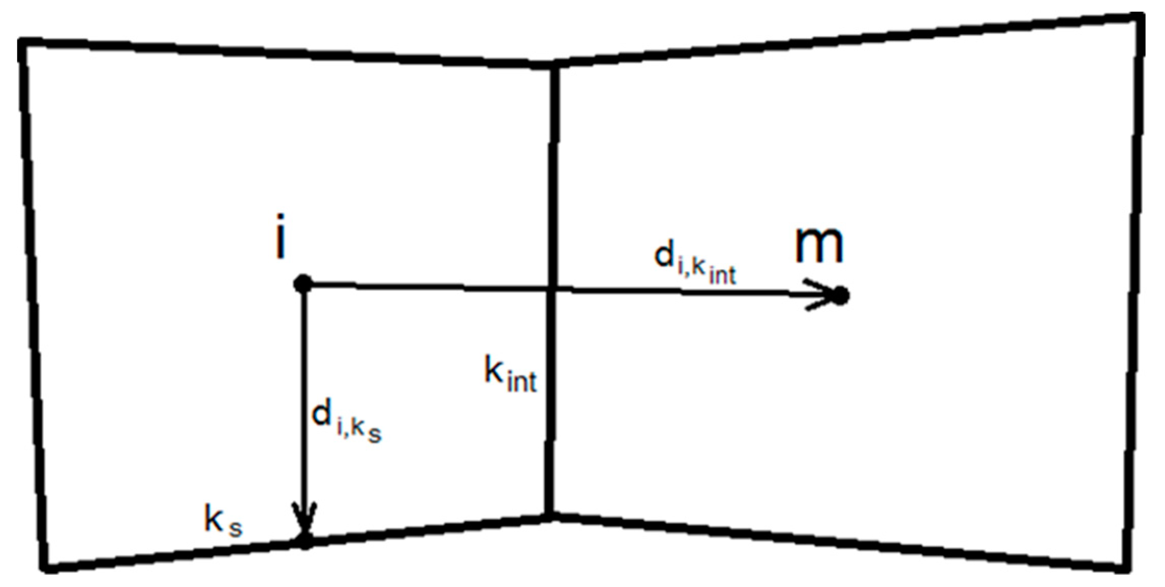
The finite-volume method provides for a transition from differentials to algebraic expressions with respect to mesh cells. Consider two adjacent cells of an unstructured mesh as shown in Figure 1.
The points i and m are the centers of the adjacent cells; k is a set of all faces of the i-th cell comprised of a set of its interior faces kint and a set of its exterior faces ks. The vector from the center of the i-th cell to the center of the m-th cell along the face kint is denoted by . The vector from the center of the i-th cell to the center of face ks is denoted by , where ri is the radius vector.
The time derivative in Equation (2) is approximated by the second-order scheme
where the superscript n denotes the time step number, the subscript i denotes the i-th cell, and Vi is the volume of the i-th cell.
The space discretization of the derivatives in Equation (1) includes their integration over the cell volume Vi and transition using the Gauss–Ostrogradsky formula to surface integrals, which are then represented as a sum of volume fluxes across the faces:
where Sj,k is the surface area of the face k and Fk is the volume flux across the face k of the i-th cell. The value of the quantity φk is determined by the numerical scheme being used.
The discretization of the diffusion term in Equation (2) is performed using the over-relaxed approach [35], which serves for non-orthogonal mesh discretization. As a result of the discretization, the diffusion term takes the form
where dk,j is the distance from the cell center to the face k; ; .
This set of equations must be supplemented by boundary conditions. For an incompressible flow, if the boundary of the computational domain consists of solid walls, all the velocity components at the boundary must be taken as equal to their corresponding velocity components of the solid surface; i.e., the fluid can neither slip along the fluid/solid interface nor move normally to it. The velocity and shear stresses at the fluid/fluid interface must be continuous. Air at the upper boundary has zero static pressure. The discretized equations above incorporate the following physical boundary conditions:
- –
- Inlet—incoming-flow boundary: , ;
- –
- Pressure—given-pressure boundary: , ;
- –
- Wall—rigid boundary: , ;
- –
- Symmetry—symmetry plane: , .
Thus, in its discretized form, the equation of continuity is written as
which, considering the equality and the boundary conditions, takes the final form
The convective term on the left side of momentum Equation (1), considering the boundary conditions, is expressed as
The diffusion term Equation (5) in Equation (1) takes the form
The final form of the discretized momentum equation is the following:
Here, the coefficient D denotes expression Equation (7).
The volume fraction transfer Equation (3), after discretization, takes the form
where the symbol G denotes the right side of expression Equation (3).
The approximation we use reduces the scalar quantity transfer Equation (2) to a system of linear algebraic equations formulated with respect to computational cells:
where Ai is the diagonal matrix coefficient, kint are the interior cell faces, are the off-diagonal matrix coefficients, and Ri is right-side vector component.
The discretized equivalents of Equation (1) reduced to the system of linear algebraic Equation (10) can be solved by the SIMPLE algorithm [19,32,33,34], one of the most common algorithms in computational fluid dynamics.
At the predictor step, in order to obtain the first approximation of the sought velocity field, a discrete equivalent of the momentum equation with respect to velocity is constructed without expanding the pressure gradient term. For the i-th cell, the equation takes the form
where ui is the velocity component in the i-th cell and is the velocity component in the near-boundary cell m at the face kint.
The matrix coefficients and the right-side members of the system of linear algebraic Equation (11) have the form
For the corrector step, an expression for velocity in the i-th cell must be derived from Equation (11):
where .
Interpolating velocity Equation (12) from the cells to the exterior faces using the geometric weighting factor λk:
and inserting Equation (13) into continuity Equation (1) gives
In practice, the weight λk can be determined in different ways—for example, basing it on the cell geometric center-to-face distances or the values of the diagonal coefficients Ai and Am, or letting λk = 0.5.
Equation (14) must also be discretized with respect to pressure; then, by analogy with Equation (10), it can be re-written for the i-th cell:
where is the diagonal equation coefficient, are the off-diagonal coefficients, and is a right-side vector component.
The members in the system of linear algebraic Equation (15) are as follows:
Solving Equation (15) allows us to find the pressure field, which is used to calculate the mass flux fields with the formula
Then, the predictor-corrector procedure is repeated with the updated velocity, pressure and mass flux fields until the desired accuracy is achieved.
Next, the volume fraction transfer Equation (9) is solved, which also needs to be formulated as a system of linear algebraic equations for the i-th cell:
Here, the matrix coefficients and the right-side members of the system of linear algebraic equations are equal to
where kout = kinlet ∪ kpress denotes the outgoing-flow boundary condition. This algorithm can be extended by an original method by taking into account the gravity term for free-surface flow simulations [36].
Thus, using this algorithm, Equation (1) can be solved numerically. This algorithm has been implemented in LOGOS and adapted for massively parallel computations on multiprocessor computers [19,26].
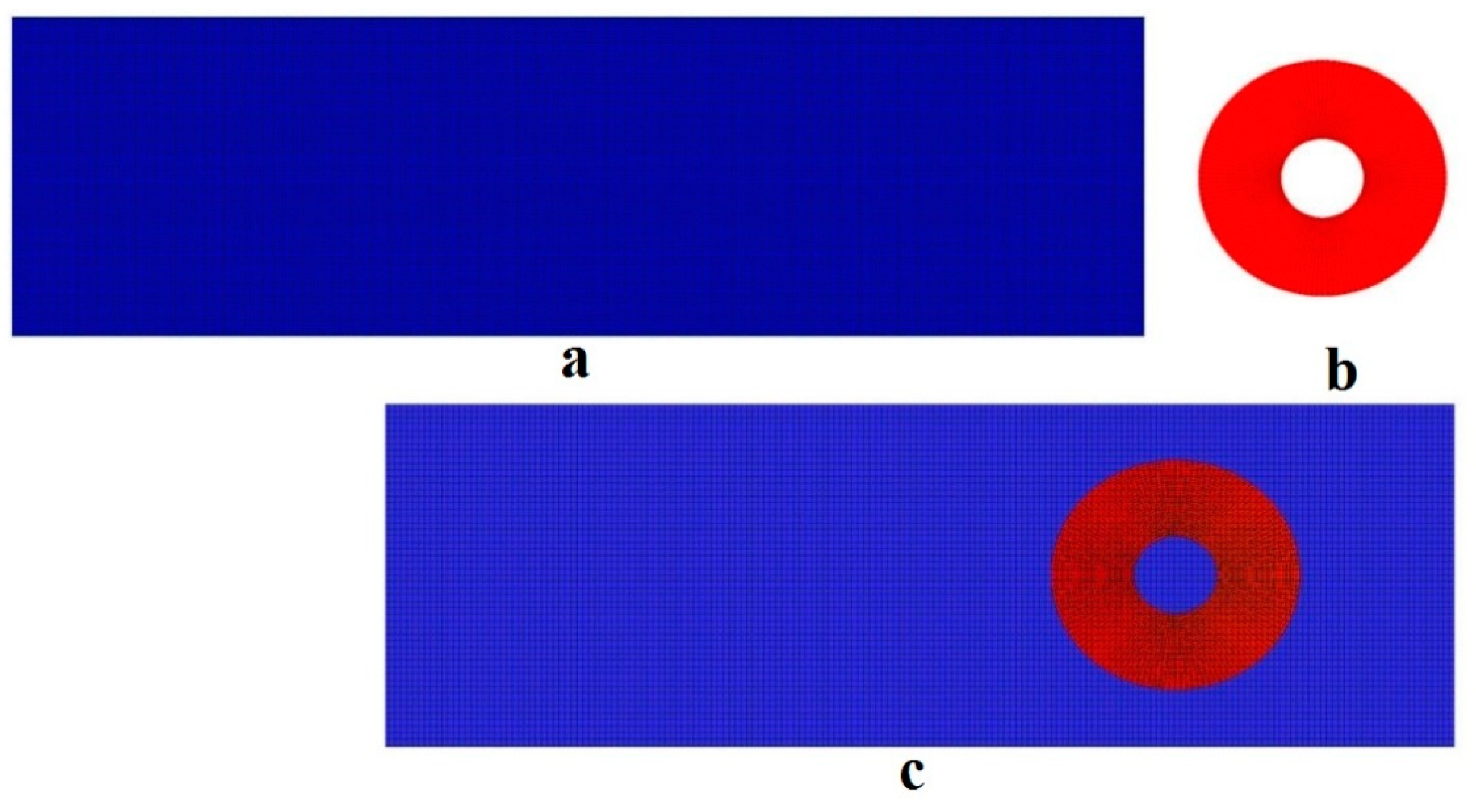
Simulations of moving bodies employ an approach based on superimposed multi-domain (Chimera) meshes [37]. In this case, the main computational domain is mapped onto a background mesh, while a separate mesh surrounding the solid body is moving atop (Figure 2). The resulting geometric models are combined into a single mesh representing the initial problem. Interaction between the background mesh and the mesh atop is implemented using an interpolation template intended to ensure correct interaction between the topologically disjoint regions.
The new interfaces generated as a result of constructing the template and tagging the cells of the combined mesh enable communication between the coupled regions and produce the required initial data for the interpolation template [36]. One of the advantages of this approach is that it allows using rather large computational domains. The mesh can be coarse in the regions far from the solid body and fine in its vicinity. Boundary tracking is performed automatically.
3. Verification Results for the LOGOS Software Package
The quantitative assessment of simulation results must be performed based on the error in calculated and experimental data at given points. Changes in the sea level caused by tsunami propagation are detected by wave gages—instruments that perform measurements and continuous computerized recording of variations in the sea level at a given accuracy. The instrumental error of wave gages can range from several millimeters to several centimeters [38]. Therefore, in wave simulations, it is reasonable to introduce a mean error and calculate it as a sum of the relative errors at each point in space or time divided by the number of such points. In some tests, we compare a wave profile relative to the experimental data, while in other cases, we evaluate the maximum value of the waveform.
Before we proceed to the verification of the tsunami simulations, let us present some results of LOGOS verification against free-surface test problems, including the collapse of a liquid column, gravity water sloshing in a tank, the fall of a sphere into a liquid, the fall of a parallelepiped into a liquid and wave flows induced by lifting a rectangular beam out of water. The verification results allow us to assess the accuracy of the predicted changes in the sea level in confined space.
3.1. Collapse of a Liquid Column
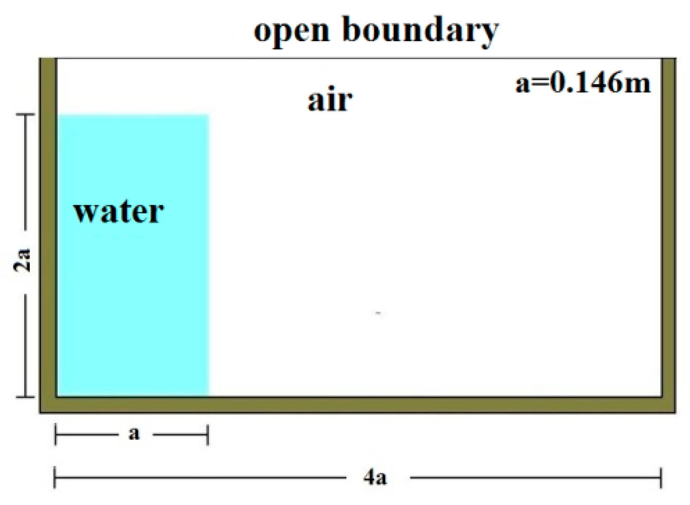
This problem considers a column of liquid (water) collapsing onto a tank bottom. The experimental results for the collapsing water column are reported in [30]. The parameters of the experimental setup and initial location of the water/air interface are shown in Figure 3.
The problem was solved using a block-structured mesh model, a mesh of uniform hexahedral cells, consisting of 8400 cells: 120 cells in the horizontal direction and 70 cells in the vertical direction; thus, ∆x = 0.033a and ∆y = 0.0286a. No-slip boundary conditions were applied to the left, right and bottom walls; the front and the back walls were slip boundaries; the top boundary had a static pressure held fixed at 0 MPa. The problem was run in single mode on an Intel Core i5 series CPU; the total computational time was approximately 10 min.
Figure 4a shows the results of the numerical modeling. The solid line represents the air/water interface, and the black dashes are the velocity vectors. The results are plotted for different time points: 0.2, 0.6 and 1.0 s. The results are presented in dimensional form as presented by Ubbink [30]. Figure 4b shows the numerical modeling results obtained in [30]. Figure 4c shows the experimental photographs [30]. By t = 0.6 s, the wave has reached the right boundary of the model (experimental) domain, and its hydraulic impact on the wall generates a wave. The time t = 0.6 s corresponds to the most active phase of collapse with the highest wave. The calculated results demonstrate an air pocket forming at the left boundary of the domain; its shape is similar in both computations. It can also be identified in the experimental photograph. At time 1.0 s, the fluid hits the left wall.
The results indicate that the calculated data qualitatively agree with the experiment in both unsteady characteristics (wave formation and collapse time) and the shape of the free surface. Figure 5 shows the time evolution of the column height along the left wall of the tank, and Figure 6 is the position of the leading edge of the liquid along the tank bottom as a function of time. The column height along the left tank wall, the position of the leading edge along the tank bottom (measured from the bottom left angle) and the time are dimensionless quantities. The solid black line represents the curves calculated in this work, the dashed line shows the results calculated in [30], and the markers represent the experimental data [30]. The mean square deviation in the calculated column height relative to the experimental data does not exceed 1%. The maximum deviation in the calculated position of the leading edge relative to the experimental data does not exceed 10%. One can see that the numerical results agree well with the experiment and the numerical solution reported in [30] both qualitatively and quantitatively.
3.2. Gravity Sloshing of Water in a Tank
The problem considers the sloshing of water in a tank under the influence of gravity. The parameters of the numerical scheme and initial interface location (water/air) are shown in Figure 7 [30].
The problem was solved using a block-structured mesh model having a size of 0.1 × 0.065 × 0.01 m and consisting of 33,600 cells, 210 cells in the horizontal direction and 160 cells in the vertical direction, resulting in ∆x = 4.762∙10−4 m and ∆y = 4.0625∙10−4 m. No-slip boundary conditions were applied to the left, right and bottom walls; the front and the back walls were slip boundaries; the top boundary had a static pressure held fixed at 0 MPa. The problem was run in single mode; the total computational time was approximately 15 min.
The numerical results for the gravity sloshing of water are presented in Figure 8. The solid line represents the water/air interface, gray shows the liquid phase, and the black dashes are the velocity vectors. The results are given for different points in time; T is the theoretical period of cosine oscillations, which is 0.3739 s in our case [30]. Panels “a” show the results obtained in [30], and panels “b”, the results calculated by LOGOS.
Initially, the interface has a cosine shape. The interface is then released and begins to slosh under the influence of gravity and liquid inertia. At t = T/4, the interface becomes horizontal, and then, at t = T/2, it recovers its cosine shape. The process is repeated in time. Figure 9 shows the time evolution of the sea level along the left wall of the tank.
Table 1 shows the time errors in the numerical results relative to the theoretical cosine oscillations. The time error is calculated as
where ts is the calculated period of oscillations and tt is the theoretical period T [30].
One can see that the numerical results are in close qualitative and quantitative agreement with the theory and the numerical solution presented in [30].
3.3. Fall of a Sphere into a Liquid
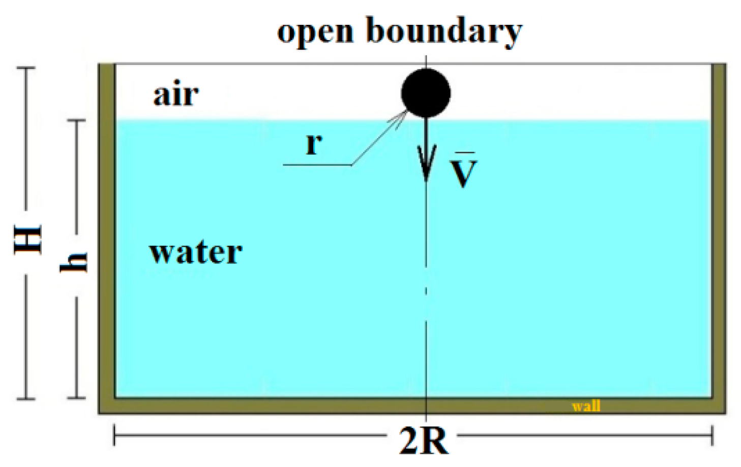
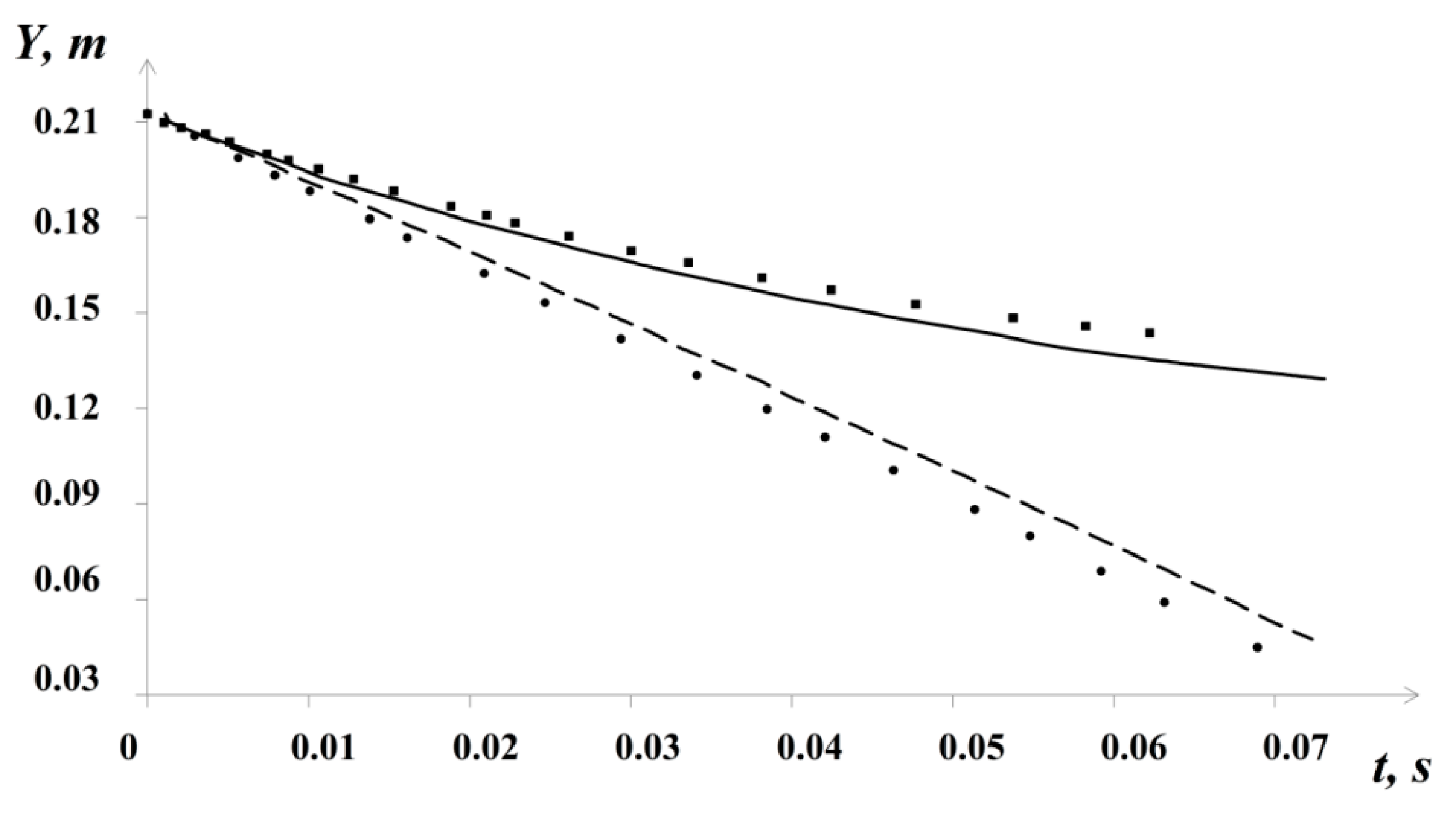
The problem simulates a fall of a solid sphere into water with low initial velocity. The experiment was conducted with spheres from different materials and reported in [39]. The problem schematic is shown in Figure 10. A sphere having a radius r = 1.27 cm and velocity V = 2.17 m/s hits the surface of water. The initial sea level h is 0.2 m. The domain is a cylinder of radius R = 0.25 m and height H = 0.2254 m.
Two computational cases were considered: in the first, the sphere was made from polypropylene, and its density was 0.86 of water’s density; in the second, the sphere was made from steel of 7.86 times water’s density.
The problem domain was discretized with a block-structured mesh model refined around the solid body and composed of 800,000 cells (see Figure 11). The cell size near the cylinder is equal to 5% of the cylinder radius. No-slip boundary conditions were applied to the wall inside a cylinder; the top boundary had a static pressure held fixed at 0 MPa. The problem was run in parallel mode on 120 standard CPUs; the total computational time was approximately 40 min.
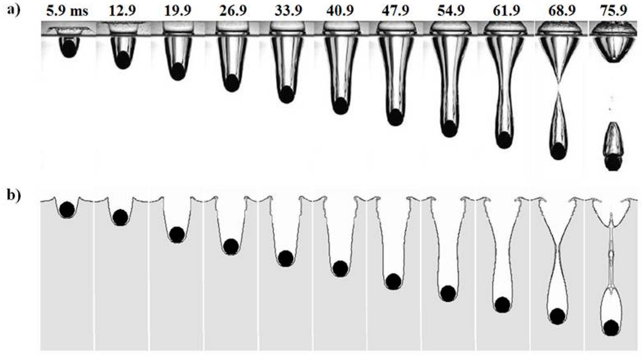
Figure 12 illustrates the descent dynamics of the steel sphere: (a) experimental photographs [39]; (b) numerical results obtained for corresponding time points. Gray represents the liquid phase, the solid black line is the interface, and the sphere is shown in black. At t = 5.9 ms, the sphere is fully submerged. At t = 54.9 ms, a cavity starts forming above the sphere. The cavity is observed to stop growing at t = 68.9 ms, both numerically and experimentally.
The numerical and the experimental results are in good qualitative agreement.
3.4. Fall of a Parallelepiped into a Liquid
The verification of the algorithm described above as applied to the description of waves traveling across a free surface can be performed by the numerical modeling of an experiment described in [24]. In the experiment, a rectangular parallelepiped of height H1 and length l falls freely from height H into water along the end wall of a tank. The tank is rectangular, with a horizontal bottom, filled with water to h < H1. In the real experiment, the tank was 4.3 m long and 0.2 m wide. In the unperturbed condition, water is quiescent. The problem geometry is shown in Figure 14.
A number of problem configurations were considered with different body dimensions, heights of fall, and water depths in the tank. These parameters have the following dimensionless form [24]:
where ρ1 and ρ are the density of the solid body and the liquid, respectively. The values of h, H0, , l0, ρ0 and x0 vary depending on the configuration.
In the first configuration, the following values were used: h = 8 cm, H0 = 3.75, = 2.26, l0 = 1.15, and ρ0 = 0.215. For the second computational configuration, h = 8 cm, H0 = 2.90, = 2.26, l0 = 0.575, and ρ0 = 0.215. A wave gage, which detects changes in the sea level, was placed at x0 = 16.
In the third configuration, h = 4 cm, H0 = 4.75, = 4.5, l0 = 1.15, and ρ0 = 0.215, and the wave gage was placed at x0 = 31.5. To model the fall of a parallelepiped into water, the 4.3 × 0.4 × 0.5 m domain was discretized with a block-structured mesh of about 20,000 cells. The mesh was refined in the regions of the fall and the wave gage. No-slip boundary conditions were applied to the left, right and bottom walls; the top boundary had zero static pressure. The experiment was run in parallel mode on 32 CPUs; the total computational time was approximately 15 min.
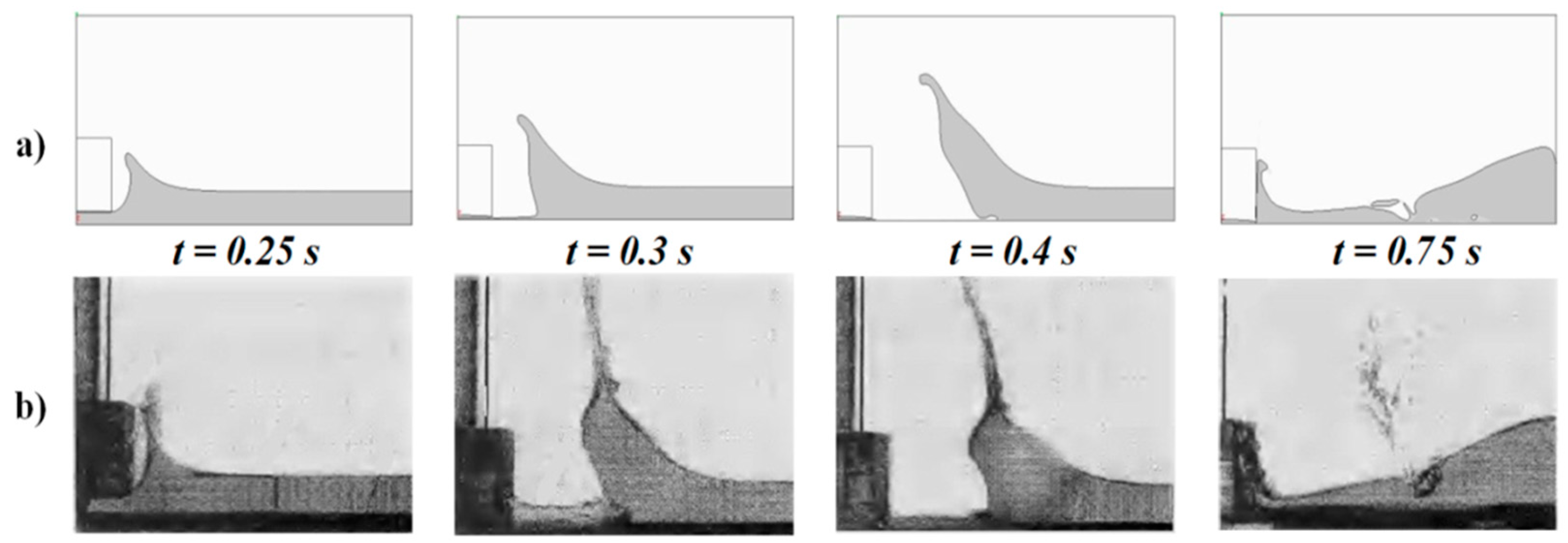
Figure 15 shows the waves produced by a falling parallelepiped in the first problem configuration. The black line is the outline of the parallelepiped. Gray represents the liquid phase. At t = 0.25 s, we observe an early phase in the development of a cavity and a splash. At t = 0.3 s, the splash continues to develop. By 0.4 s, the tank bottom becomes clear of water, and the rate of splash formation slows down. The late phase in the evolution of the cavity (its collapse) and the splash is shown at t = 0.75 s. Note that the photography time points are not specified in [24], so our numerical results were obtained for the time points chosen at our discretion.
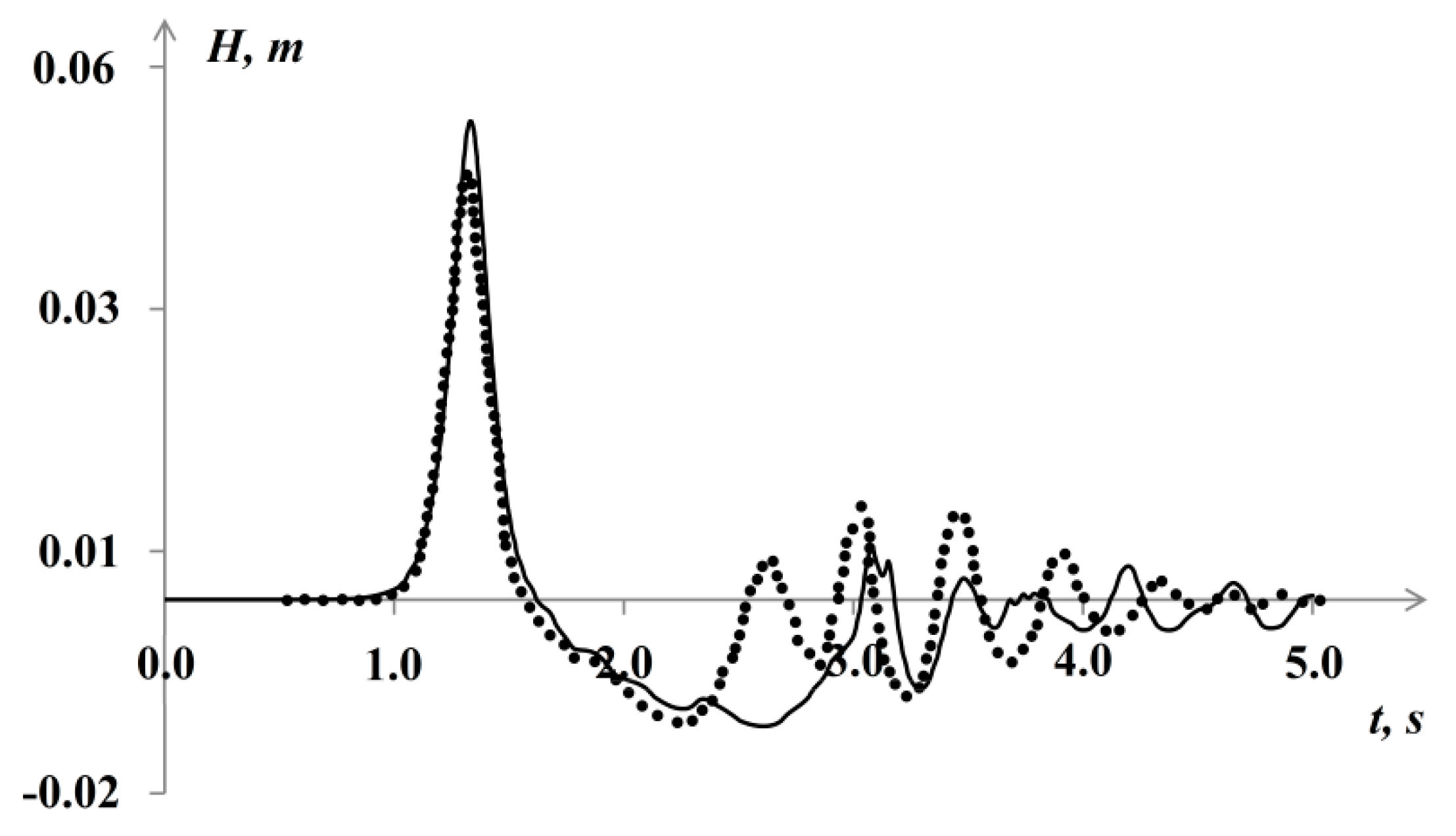
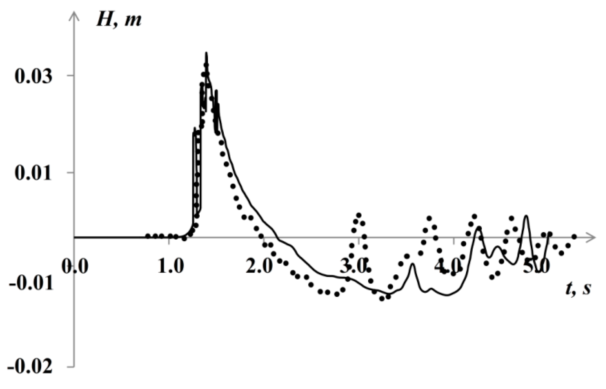
Figure 16 and Figure 17 are the amplitudes of water sloshing in the tank as a function of time for the second and the third configurations, respectively. The dots in the plot represent the experimental data measured by a fixed wave gage [24]. The solid black line shows the amplitude of water sloshing in the tank obtained in the calculations.
Comparison of the gage readings demonstrates close agreement for the first incoming wave. For the second configuration, the difference between the calculated and the experimental amplitudes of the first wave is 4%, and for the third configuration, 5%. The calculated amplitude of the second wave (“negative”) also closely matches the experimental data, but a difference is observed in subsequent surface oscillations of millimeter amplitude.
3.5. Wave Flows Induced by Lifting a Beam Partially Immersed into Shallow Water
This problem considers the lifting of a solid body from the surface of a liquid and associated wave flows [25]. The problem geometry (Figure 18) is a horizontal-bottom rectangular prismatic channel with a beam partially immersed into shallow water. The modeling was performed without friction and the surface tension of water, whose viscosity was taken as equal to 10−6.
The rectangular channel is filled with an incompressible liquid, into which a beam is partially immersed. The beam has length 2L, where L = 1 m, and the same width as the channel. The channel depth is h0 = 20 cm, and the depth under the beam is h1 = 5 cm. Both the liquid and the beam are initially at rest. The beam is lifted out of water at a constant velocity of 7.5 cm/s.
The beam motion is simulated using an approach based on superimposed multi-domain (Chimera) meshes. According to this technique, the mesh is divided into a background mesh, covering all the computation domain, and an overset mesh, representing the domain of a moving body [37]. The problem domain was discretized with an unstructured computational mesh consisting of truncated polyhedrons (Figure 19). Highlighted in Figure 19 is the superimposed mesh. The mesh had ~30,000 cells, and its basic size was 0.02 m. Next to the liquid surface, an additional refined block was constructed with a mesh size of ∆y = 0.005 m. The experiment was carried in parallel mode on 16 CPUs; the total computational time was approximately 20–30 min.
Figure 20 shows the pictures of wave propagation as a result of lifting the beam at different time points.
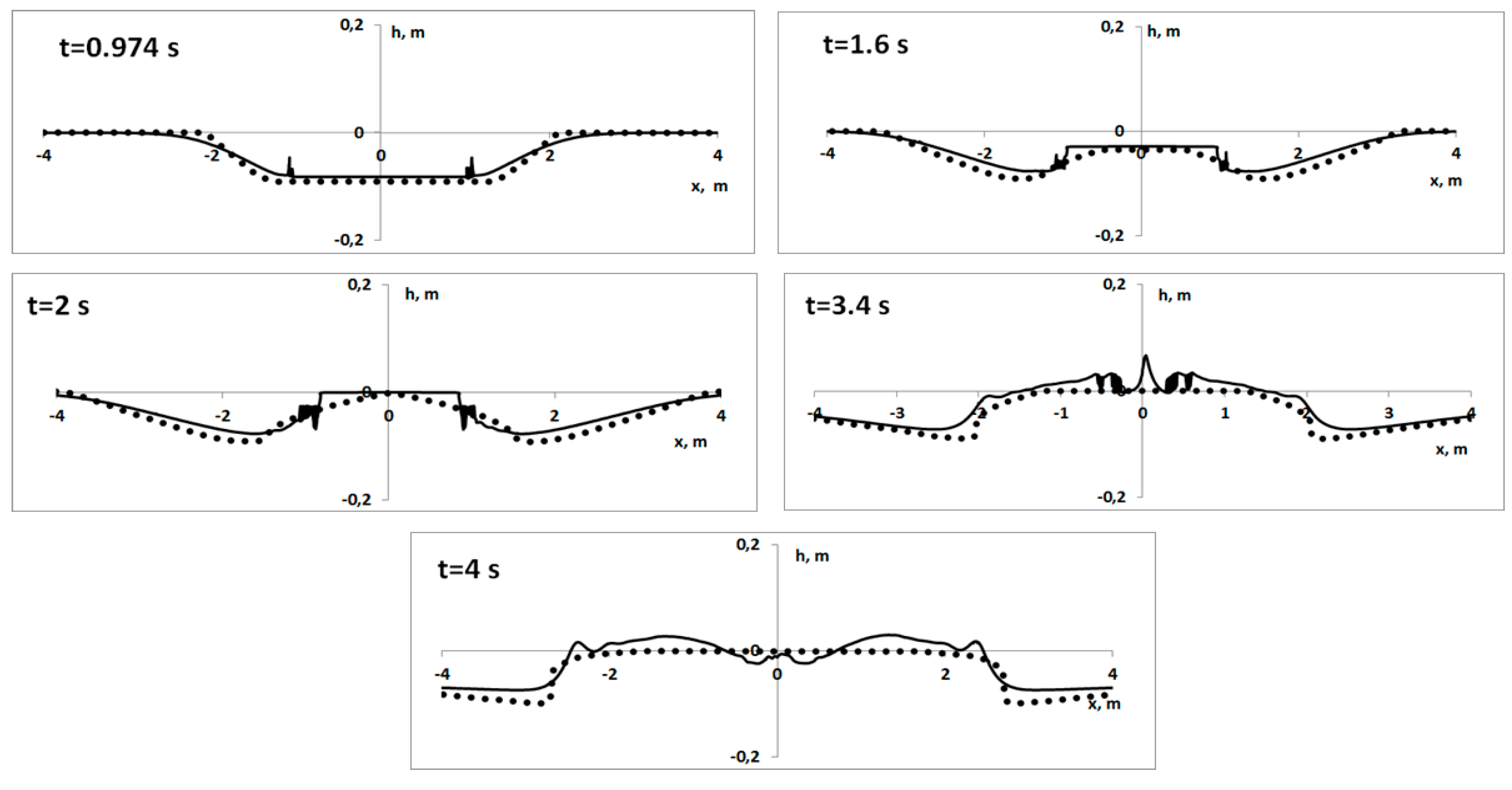
Figure 21 shows the wave profiles at different time points. The results calculated by LOGOS are compared with data obtained in [25]. The mean square deviation with respect to the reference numerical data for this test case does not exceed 7%.
The diagrams demonstrate that the results are in close agreement. When the bottom of the beam is fully under water, depression waves are propagating across the region beyond the beam. Then, when the beam is lifted, the sea level under it increases, producing a flow directed towards the beam center. Once the beam is detached from water, two diverging waves are produced.
3.6. Propagation and Run-Up of a Single Wave over a Flat Slope
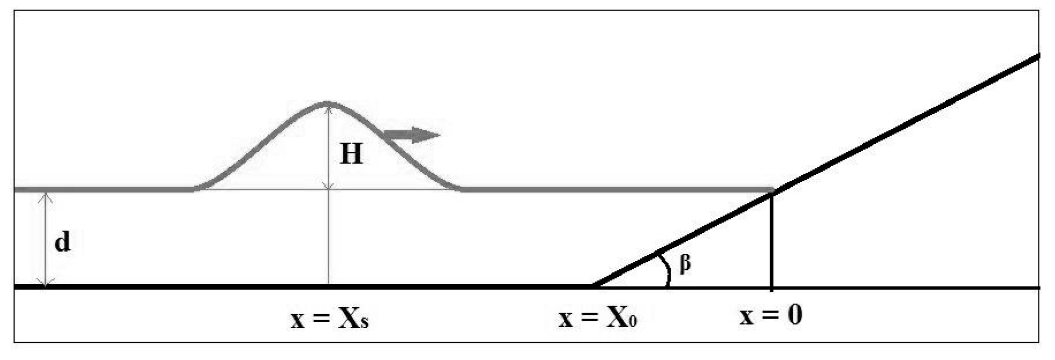
This problem simulates a single wave of height H propagating in a tank of constant depth d = 1 m [22] and then running up over a slope of angle β = 2.88°. The schematic representation of the tank configuration is shown in Figure 22. This problem was proposed in [22] as a benchmark.
The study [22] considers several problem configurations with different H/d ratios. In the first case, H/d = 0.0185, and in the second, H/d = 0.3. The initial waveform of the wave is defined by
where . The initial velocity of the wave is , which, in the framework of the linear shallow-water theory, ensures that the wave is propagating to the right.
The problem was simulated on a mesh composed of 200,000 cells (Figure 23). The technology of mesh model construction for tsunami simulations is described in detail in [19]. The mesh is refined near the wave run-up over the slope and toward the interface to resolve the details of wave propagation. The problem was run in parallel mode on 64 standard CPUs; the total computational time was approximately 20 min.
The parameters of both the water and air phases are given in Table 2.
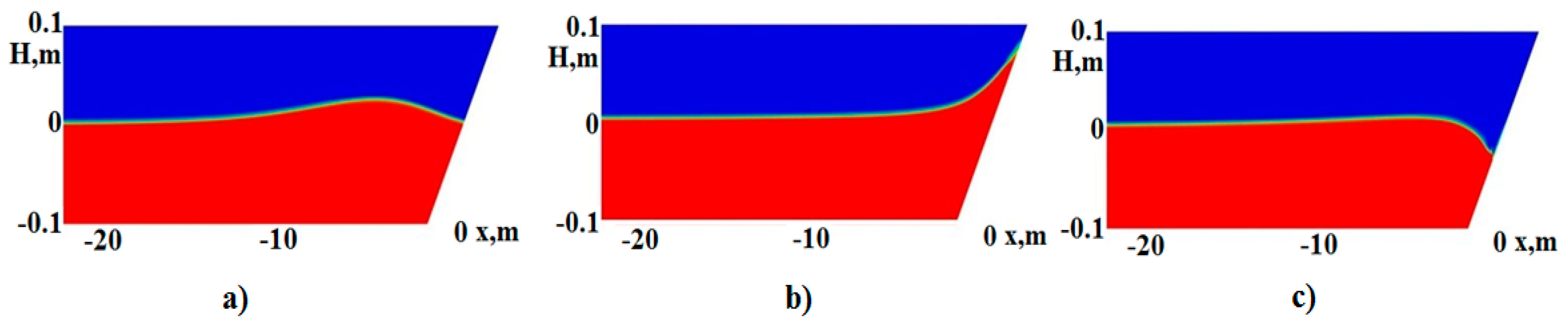
Figure 24 shows the positions of the free surface at dimensionless time points for the first problem configuration, where τ is an actual physical time.
The light color shows the mixed cells containing both air and water. This layer is thin.
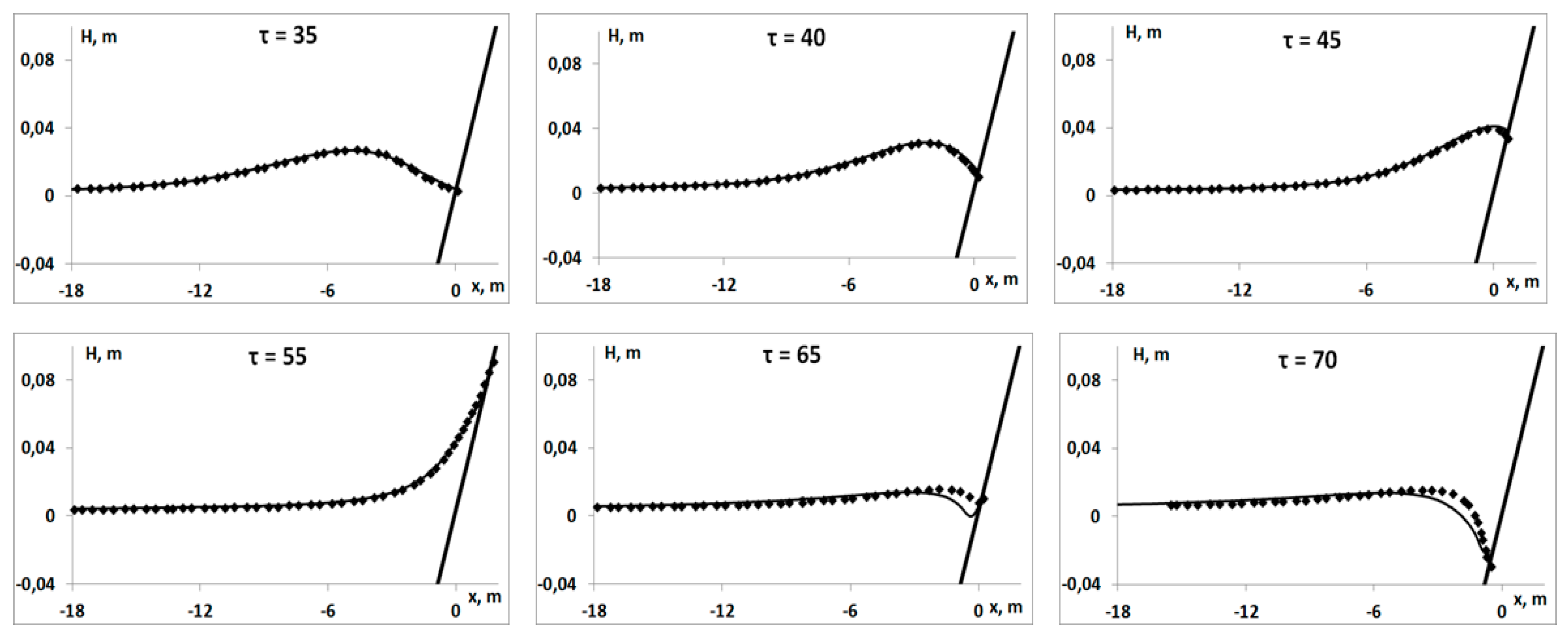
The waveforms of the wave calculated by LOGOS were compared with the analytical data [22]. Figure 25 shows the comparisons for the first configuration (H/d = 0.0185) at different time points .
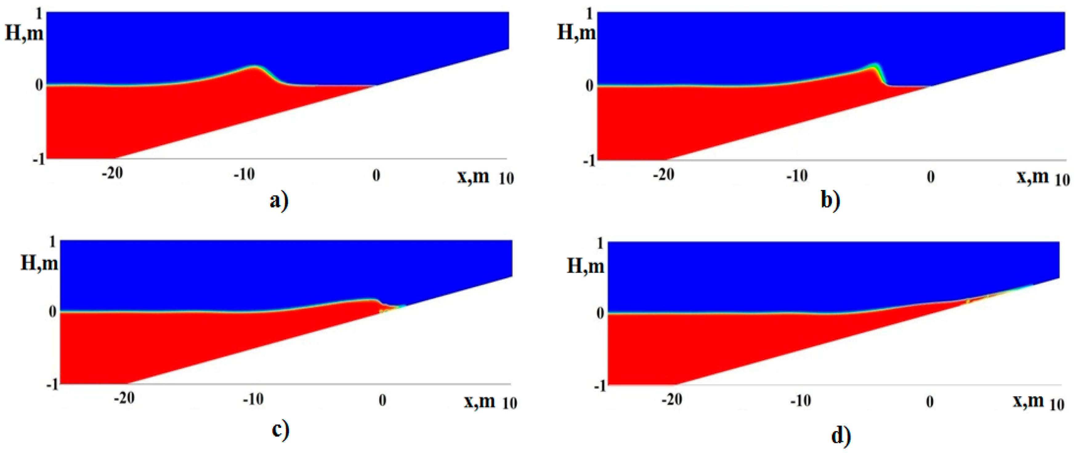
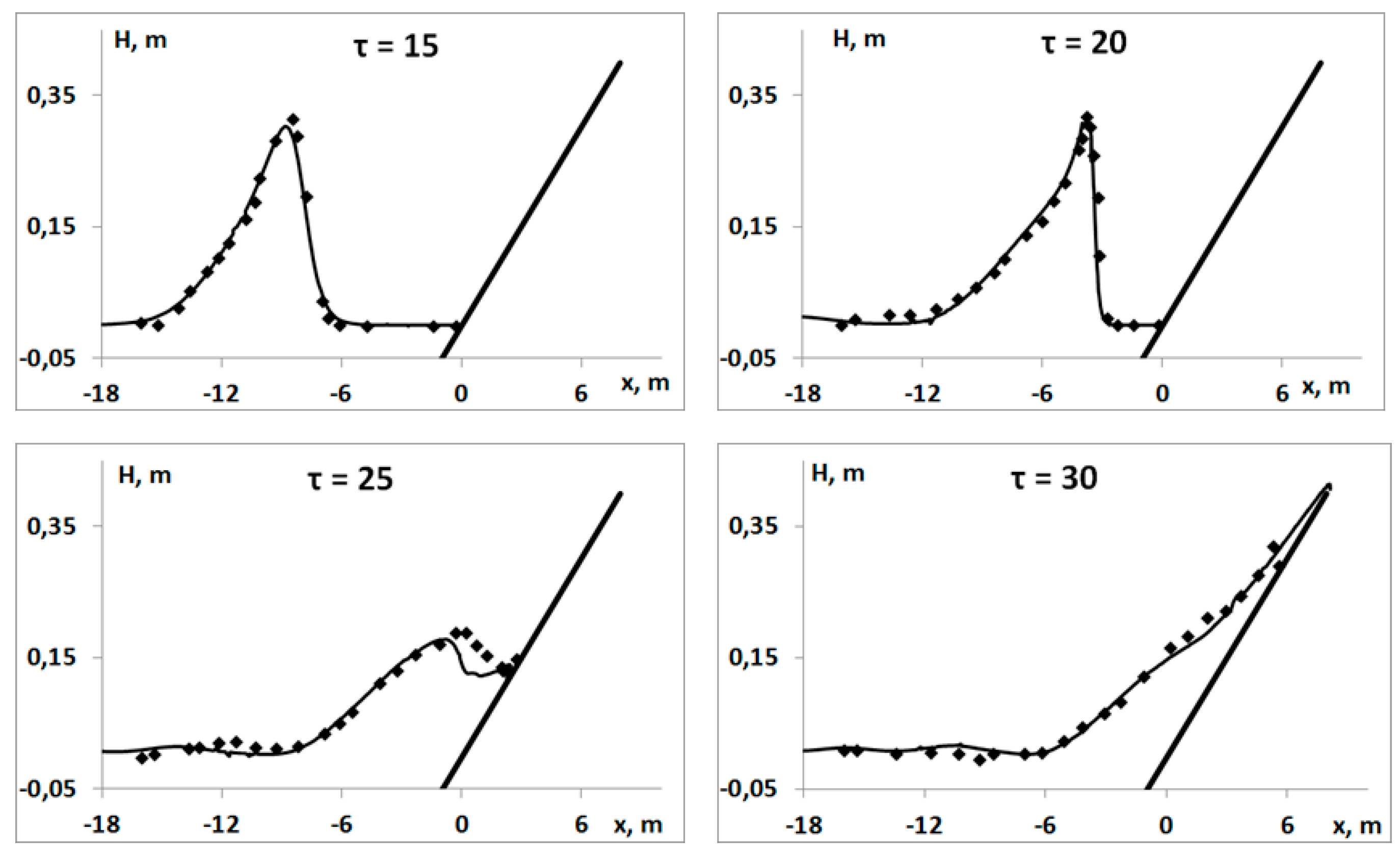
Figure 26 shows positions of the free surface at different time points for the second configuration. Figure 27 shows data comparisons for the second configuration (H/d = 0.3) at different time points.
The numerical results demonstrate close agreement with the analytical data: The single wave moves while preserving its amplitude until it reaches the slope, runs up onto the slope and washes back. The results calculated by LOGOS consistently describe both the propagation of the wave and its run-up over the slope.
3.7. Propagation and Run-Up of a Single Wave in a Varied-Depth Basin
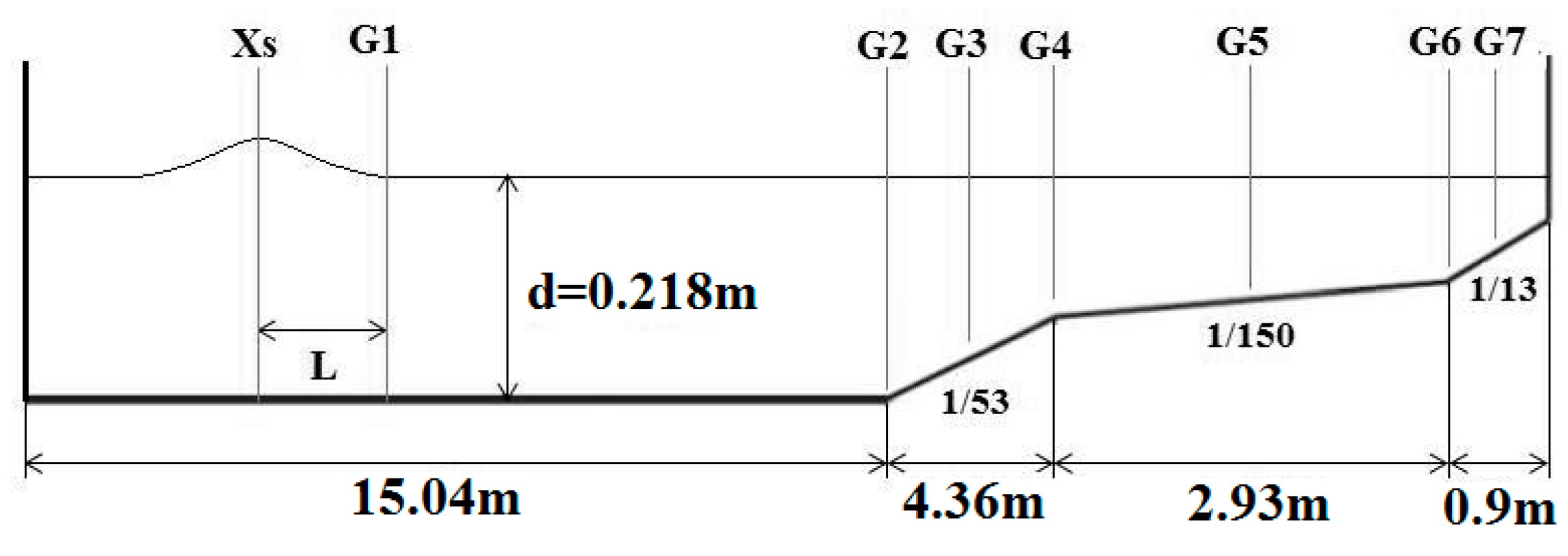
The problem simulates a single wave propagating in a basin of varied depth [22]. The configuration and the dimensions of the basin are shown in Figure 28.
In the reference, three problem configurations are considered with different ratios of wave height H to basin depth d. In the first case, H/d = 0.038 and L = 2.4 m; in the second case, H/d = 0.259 and L = 0.98 m; in the third case, H/d = 0.681 and L = 0.64 m. The spacing between wave gages G1 and G2 is 2.4, 0.98 and 0.64 m in the first, second and third cases, respectively. The initial waveform of the wave is given by Equation (17).
The problem was simulated on a computational mesh of 160,000 cells. The mesh was refined towards the interface to provide more accurate simulation. The cell height was chosen such that there were at least 10 cells along the wave height and at least 20 cells along the wavelength. The parameters of both the water and air phases are given in Table 2.
The calculated quantitative characteristics of the wave pattern in the basin can be evaluated based on the wave gage data. LOGOS calculations were performed for all the problem configurations. To demonstrate that the problem solution is correct, let us compare the numerical results with the analytical data for the first problem configuration (Figure 29). The results for the two other configurations look similar.
Figure 29 shows that the numerical results, both qualitatively and quantitatively, closely match the analytical data. Both the wave incident on the wave gage and the reflected wave are described well. The wave propagates with the same velocity as in the experiment. The maximum deviation in the calculated amplitudes does not exceed 4% for the incoming wave and 13% for the reflected wave at wave gage G6. This error is satisfactory for tsunami simulations.
3.8. Single Wave Flowing around a Conical Island
This problem serves for numerically modeling an experiment described in [22,40]. In this experiment, a single wave was produced by a wave maker in a basin of length 25 m and width 30 m filled with water to 0.32 m. The wave flowed around an island of a regular truncated conical shape having a height of 0.625 m, a bottom base diameter of 7.2 m and a top base diameter of 2.2 m. The basin walls were lined with an absorbing material to minimize wave reflection. Changes in the sea level were recorded by means of gages. The problem geometry and locations of the reference gages are shown in Figure 30.
Two problem configurations with different wave heights were considered. For the first case, H = 0.016 m; for the second case, H = 0.032 m. The initial waveform of the wave is given by Equation (17).
The problem was solved using a computational mesh refined at the interface and composed of 1.4 million cells. The base cell size is equal to 0.08 m; the vertical cell size near the interface is equal to 0.005 m. The basin walls in the discrete model were non-reflecting boundaries, through which waves could leave the domain without reflection; the bottom and the island were no-slip boundaries; and the top boundary had fixed zero static pressure. The experiment was run in parallel mode on 128 CPUs; the total computational time was about 60 min.
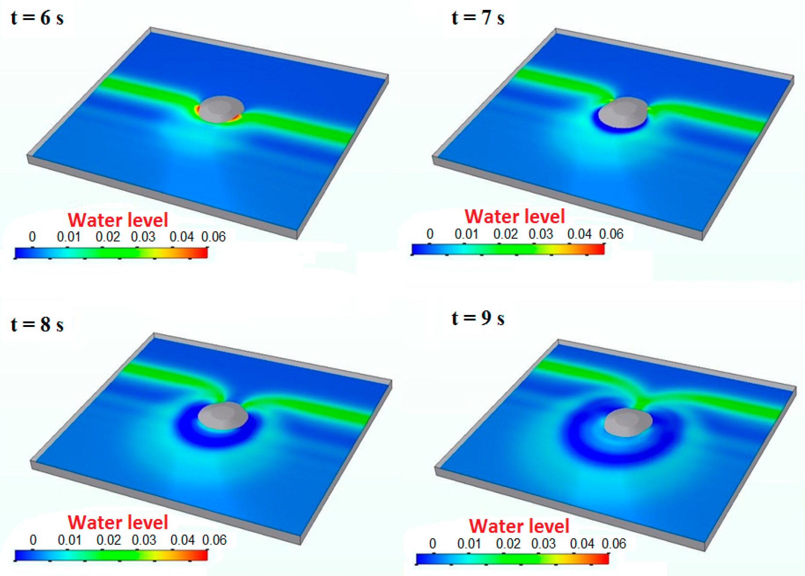
Figure 31 shows the calculated results for a wave flowing around an island at individual time points.
The calculated results show that the wave pattern of the flow around the island corresponds to the classical description of a flow with a detached boundary layer around a bluff-stern body [41].
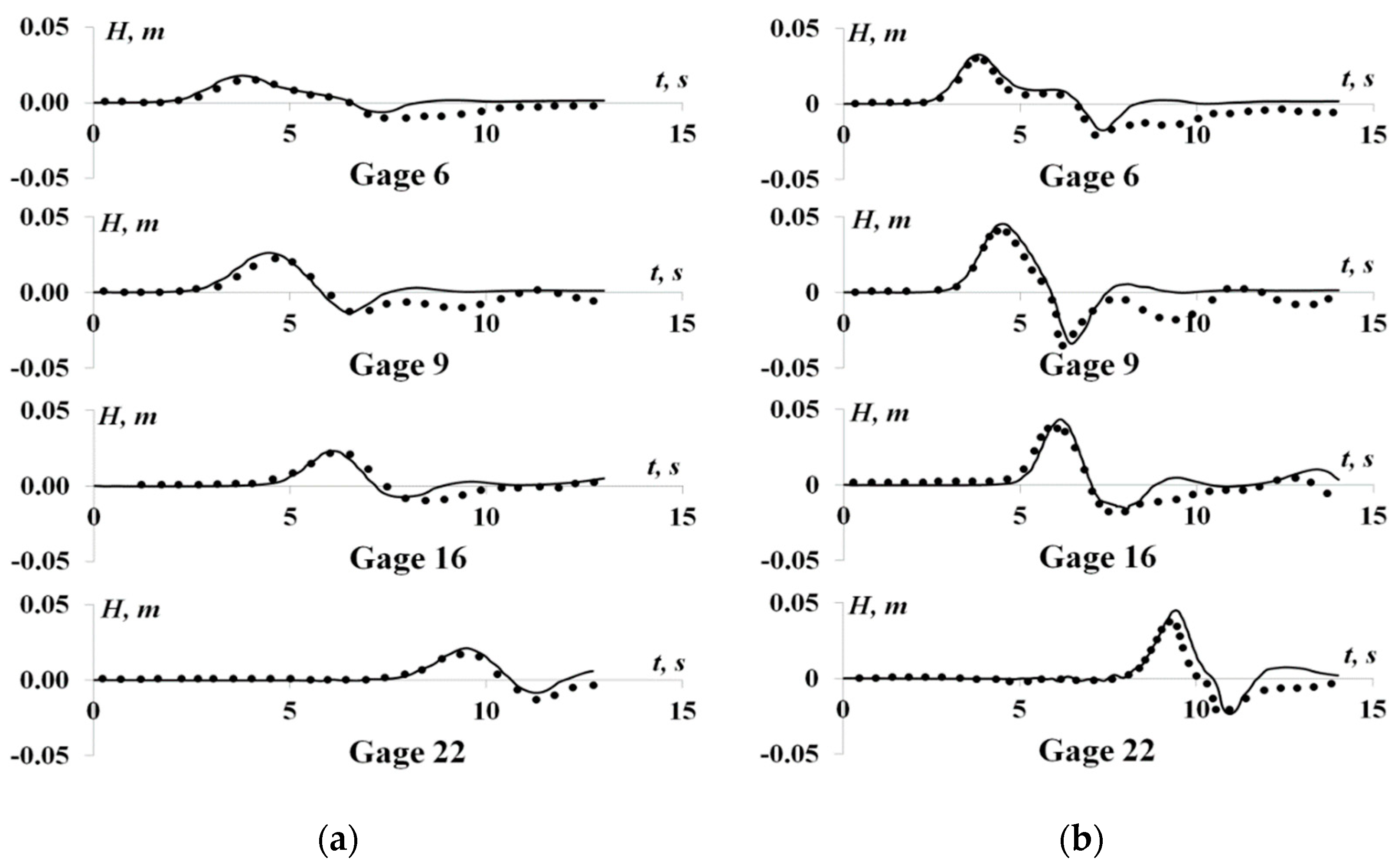
Figure 32 shows the amplitude of water sloshing in the basin as a function of time for the two problem configurations. The dots in the plot represent the experimental data from [40]. The solid black line shows the amplitude of water sloshing in the basin obtained in the LOGOS calculations.
Comparison of the gage readings shows their close agreement for the first incident wave both in the waveform and in the amplitude of the wave. However, some differences in further sloshing are observed, which can be related to the mesh quality. The mean square deviation relative to the analytical solution for this problem is about 10%.
3.9. Generation of Waves by a Sliding Wedge-Shaped Body
This problem serves for numerically modeling an experiment described in [22,42]. In this experiment, waves were generated by a wedge-shaped body of height 0.455 m, length 0.91 m and width 0.61 m sliding under the influence of gravity down a slope in a tank with water (Figure 33). The problem geometry and gage locations are shown in Figure 33. All the dimensions are given in meters.
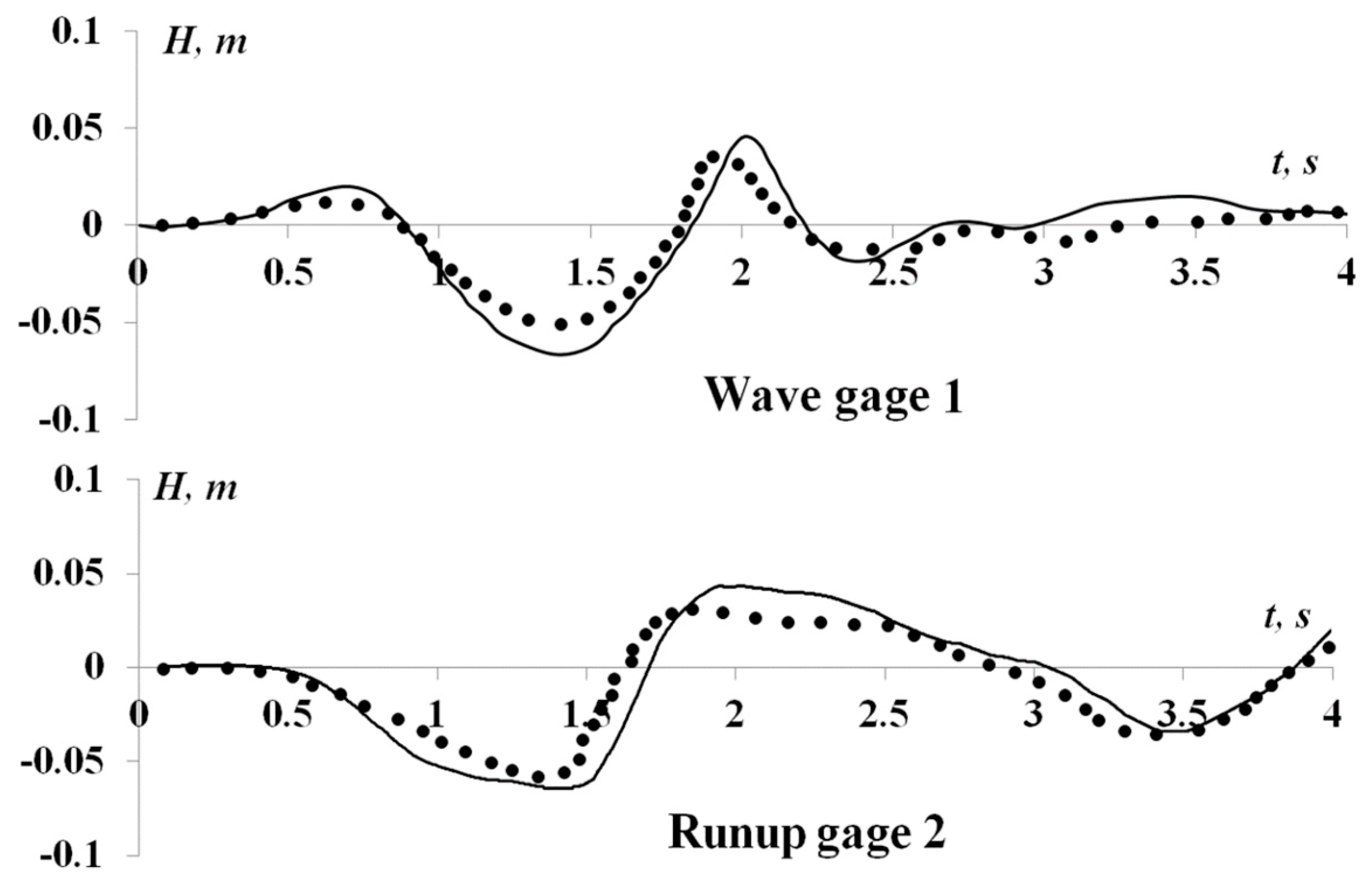
Gage 1 measures the change in sea level, and Gage 2, the run-up over the slope.
The problem was solved using a composite computational mesh (Figure 34) refined at the interface and wave propagation area and composed of 2.5 million cells, including a prismatic sublayer on the slope. The base cell size is equal to 0.02 m. The walls and the bottom of the tank were no-slip boundaries; the top boundary had fixed zero static pressure. The problem was run in parallel mode on 96 CPUs; the total computational time was 70 min.
Figure 35 shows the waves generated by the sliding wedge.
The numerical modeling confirms that the sea level behind the wedge-shaped body sliding down along a slope is depressed, following which a diverging wave forms. Figure 36 shows the wave amplitude as a function of time for Gages 2 and 4.
The plots in Figure 36 demonstrate close quantitative agreement between the numerical and the experimental data. Here, we estimate the waveform relative to the experiment; the mean error, taken as the mean value of the errors corresponding to the given experimental points, for this problem is about 15%.
3.10. Wave Propagation in a Nonuniform-Bottom Tank with Run-Up onto an Obstacle
This problem considers a wave traveling across a basin of length 22 m and depth h0 = 0.2 m. The bottom of the basin starting from x = 10 m has a slope and an obstacle. Experimental studies of such wave propagation are reported in [23]. This problem is a good test to verify the technique described above.
Figure 37 shows the problem geometry. The wave is formed at the left wall of the basin and has a height of H0 = 0.07 m.
Elevation coordinates of the obstacle are given in Table 3.
The problem domain was discretized with a three-dimensional unstructured computational mesh consisting of truncated polyhedrons (Figure 38).
The mesh had 1.1 million cells. The characteristic cell size was set as 0.1 m. To resolve the moving wave in greater detail, an additional mesh block was constructed with refinement around y = 0 from −0.1 to 0.2 m, where the characteristic size was ∆x = 0.02 m and ∆y = 0.001 m. The problem was run in parallel mode on 64 CPUs; the total computational time was 20 min.
Figure 39 shows the wave profiles calculated by LOGOS in comparison with the experiment at different time points. One can see that the calculated and the experimental data are in close agreement.
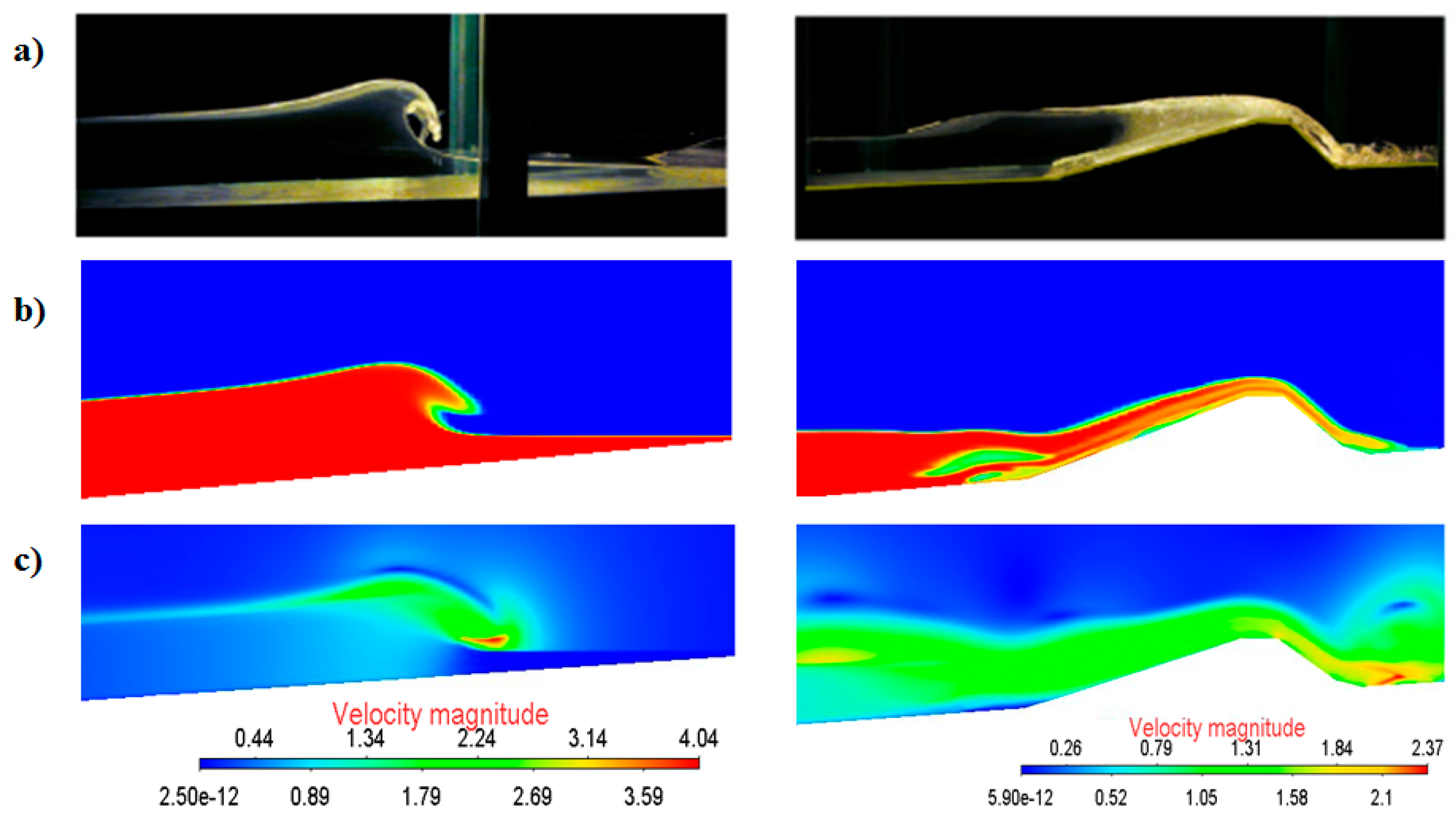
Figure 40 presents a comparison of the calculated wave profiles with the experimental data and calculated velocity fields.
The results shown in the figure demonstrate close qualitative agreement between the calculated and the experimental data.
4. Conclusions
The paper presents verification results for the LOGOS software package as applied to tsunami simulations. First, LOGOS free-surface flow simulations were verified against the test cases of a collapsing water column and gravity water sloshing in a tank and the known test cases of wave generation by objects falling into water or lifted out of it. Then, LOGOS verification specifically as applied to tsunami simulations was performed on international benchmarks, including the propagation and run-up of a single wave onto a flat slope and a vertical wall, the sliding of a wedge-shaped body down a slope, flow around an island and wave run-up onto an obstacle.
The results of the verification calculations show that LOGOS enables sufficiently accurate numerical simulations of free-surface flows and delivers acceptable results in tsunami simulations. LOGOS is shown to be good at modeling the formation, propagation and run-up of waves. For all the problems, the error in the calculated results relative to the reference data does not exceed 10%, except for one problem, in which the error was 15%. This level of accuracy is satisfactory for tsunami simulations. Consequently, this technology can be used in numerical simulations of tsunami propagation, including generation, propagation and run-up on a beach.
Author Contributions
Conceptualization, A.K. (Andrey Kozelkov), A.K. (Andrey Kurkin) and E.P.; data curation, E.T., V.K., K.P. and D.U.; formal analysis, A.K. (Andrey Kozelkov) and V.K.; investigation, E.T., A.K. (Andrey Kozelkov), A.K. (Andrey Kurkin), E.P., V.K., K.P. and D.U.; methodology, A.K. (Andrey Kozelkov), A.K. (Andrey Kurkin), E.P. and V.K.; software, E.T., V.K., K.P. and D.U.; supervision, A.K. (Andrey Kurkin); validation, E.T., K.P. and D.U.; visualization, E.T., K.P. and D.U.; writing—original draft, A.K. (Andrey Kozelkov), A.K. (Andrey Kurkin) and E.P. All authors have read and agreed to the published version of the manuscript.
Funding
The research was supported by grants of the President of the Russian Federation for the state support of research projects by leading scientific schools of the Russian Federation (NSh-2485.2020.5) and by the Russian Foundation for Basic Research (20-05-00162).
Conflicts of Interest
The authors declare no conflict of interest.
References
- Horspool, N.; Pranantyo, I.R.; Griffin, J.; Latief, H. A probabilistic tsunami hazard assessment for Indonesia. Nat. Hazards Earth Syst. Sci. 2017, 14, 3105–3122. [Google Scholar] [CrossRef] [Green Version]
- Løvholt, F.; Griffin, J.; Salgado-Gálvez, M.A. Tsunami Hazard and Risk Assessment on the Global Scale. In Encyclopedia of Complexity and Systems Science; Meyers, R.A., Ed.; Springer Science+Business Media: New York, NY, USA, 2016; pp. 1–34. [Google Scholar] [CrossRef]
- Okumura, N.; Jonkman, S.N.; Esteban, M.; Hofland, B.; Shibayama, T. A method for tsunami risk assessment: A case study for Kamakura, Japan. Nat. Hazards 2017, 88, 1451–1472. [Google Scholar] [CrossRef] [Green Version]
- Ohori, M.; Masukawa, Y.; Kojima, K. Tsunami Hazard Assessment for the Hokuriku Region, Japan: Toward Disaster Mitigation for Future Earthquakes. In Natural Hazards: Risk Assessment and Vulnerability Reduction; do Carmo, J.S.A., Ed.; IntechOpen: London, UK, 2018. [Google Scholar] [CrossRef] [Green Version]
- Nosov, M.A.; Kolesov, S.V. Combined Numerical Model of Tsunami. Math. Models Comput. Simul. 2019, 11, 679–689. [Google Scholar] [CrossRef]
- Shokin, Y.I.; Gusiakov, V.K.; Kikhtenko, V.A.; Chubarov, L.B. Tsunami hazard mapping methodology and its implementation for the Far Eastern coast of the Russian Federation. Dokl. Earth Sci. 2019, 489, 419–423. [Google Scholar] [CrossRef]
- Kozelkov, A.S.; Kurkin, A.A.; Pelinovsky, E.N.; Kurulin, V.V.; Tyatyushkina, E.S. Numerical modeling of the 2013 meteorite entry in Lake Chebarkul, Russia. Nat. Hazards Earth Syst. Sci. 2017, 17, 671–683. [Google Scholar] [CrossRef] [Green Version]
- Grilli, S.T.; Tappin, D.R.; Carey, S.; Watt, S.F.L.; Ward, S.N.; Grilli, A.R.; Engwell, S.L.; Zhang, C.H.; Kirby, J.T.; Schambach, L.; et al. Modelling of the tsunami from the December 22, 2018 lateral collapse of Anak Krakatau volcano in the Sunda Straits, Indonesia. Sci. Rep. 2019, 9, 11946. [Google Scholar] [CrossRef]
- Levin, B.W.; Nosov, M.A. Physics of Tsunamis; Springer International Publishing: Cham, Switzerland, 2016; 388p. [Google Scholar] [CrossRef]
- Kozelkov, A.; Pelinovsky, E. Tsunami of the meteoritic origin. In Dynamics of Disasters–Key Concepts, Models, Algorithms, and Insights; Kotsireas, I.S., Nagurney, A., Pardalos, P.M., Eds.; Springer: Berlin, Germany, 2016; Volume 185, pp. 135–157. [Google Scholar] [CrossRef]
- Badescu, V.; Isvoranu, D. Dynamics and Coastal Effects of Tsunamis Generated by Asteroids Impacting the Black Seа. Pure Appl. Geophys. 2011, 168, 1813–1834. [Google Scholar] [CrossRef]
- Pelinovsky, E.N. Hydrodynamics of Tsunami Waves; Institute of Applied Physics: Nizhny Novgorod, Russia, 1996; 276p. (In Russian) [Google Scholar]
- Goto, C.; Ogawa, Y.; Shuto, N.; Imamura, N. Numerical Method of Tsunami Simulation with the Leap-Frog Scheme; IUGG/IOC Time Project, IOC Manual, No. 35; UNESCO: Paris, France, 1997; 96p. [Google Scholar]
- Kirby, J.; Wei, G.; Chen, Q.; Kennedy, A.; Dalrymple, R. Fully Nonlinear Boussinesq Wave Model. Documentation and Users Manual; Research Report №CACR-98-06; University of Delaware: Newark, NJ, USA, 1998. [Google Scholar]
- Yalciner, A.; Pelinovsky, E.; Talipova, T.; Kurkin, A.; Kozelkov, A.; Zaitsev, A. Tsunamis in the Black Sea: Comparison of the historical, instrumental and numerical data. J. Geophys. Res. 2004, 109, 1–13. [Google Scholar] [CrossRef]
- Landau, L.D.; Lifshitz, E.M. Fluid Mechanics; Pergamon Press: Oxford, UK, 1987. [Google Scholar]
- Horrillo, J.; Wood, A.; Kim, G.B.; Parambath, A. A simplified 3-D Navier-Stokes numerical model for landslide-tsunami: Application to the Gulf of Mexico. J. Geophys. Res. Ocean. 2013, 118, 6934–6950. [Google Scholar] [CrossRef]
- Kozelkov, A.S.; Kurkin, A.A.; Pelinovskii, E.N.; Kurulin, V.V. Modeling the Cosmogenic Tsunami within the Framework of the Navier–Stokes Equations with Sources of Different Types. Fluid Dyn. 2015, 50, 306–313. [Google Scholar] [CrossRef]
- Kozelkov, A.S. The Numerical Technique for the Landslide Tsunami Simulations Based on Navier-Stokes Equations. J. Appl. Mech. Tech. Phys. 2017, 58, 1192–1210. [Google Scholar] [CrossRef]
- Roache, P.J.; Ghia, K.; White, F. Editorial Policy Statement on the Control of Numerical Accuracy. ASME J. Fluids Eng. 1986, 108, 2. [Google Scholar] [CrossRef] [Green Version]
- American Institute of Aeronautics and Astronautics. Guide for the Verification and Validation of Computational Fluid Dynamics Simulations; G-077-1998; American Institute of Aeronautics and Astronautics: Reston, VA, USA, 1998. [Google Scholar]
- National Tsunami Hazard Mitigation Program. In Proceedings of the 2011 NTHMP Model Benchmarking Workshop, Galveston, TX, USA, 31 March–1 April 2011; U.S. Department of Commerce: Boulder, CO, USA, 2012.
- Hsiao, S.-C.; Lin, T.-C. Tsunami-like solitary waves impinging and overtopping an impermeable seawall: Experiment and RANS modeling. Coast. Eng. 2010, 57, 1–18. [Google Scholar] [CrossRef]
- Bukreev, V.I.; Gusev, A.V. Gravity waves generated by a body falling onto shallow water. J. Appl. Mech. Tech. Phys. 1996, 37, 224–231. [Google Scholar] [CrossRef]
- Ostapenko, V.V.; Kovyrkina, O. Wave flows induced by lifting of a rectangular beam partly immersed in shallow water. J. Fluid Mech. 2017, 816, 442–467. [Google Scholar] [CrossRef]
- Kozelkov, A.S.; Kurulin, V.V.; Lashkin, S.V.; Shagaliev, R.M.; Yalozo, A.V. Investigation of Supercomputer Capabilities for the Scalable Numerical Simulation of Computational Fluid Dynamics Problems in Industrial Applications. Comput. Math. Math. Phys. 2016, 56, 1506–1516. [Google Scholar] [CrossRef]
- Kozelkov, A.S.; Kurulin, V.V. Eddy resolving numerical scheme for simulation of turbulent incompressible flows. Comput. Math. Math. Phys. 2015, 5, 1255–1266. [Google Scholar] [CrossRef]
- Volkov, K.N.; Deryugin, Y.N.; Kozelkov, A.S.; Emelyanov, V.N.; Teterina, I.V. Difference Schemes in Gas Dynamic Simulations on Unstructured Meshes; Fizmatlit: Moscow, Russia, 2014; 416p. (In Russian) [Google Scholar]
- Hirt, C.W.; Nichols, B.D. Volume of Fluid (VOF) method for the dynamics of free boundaries. J. Comput. Phys. 1981, 39, 201–225. [Google Scholar] [CrossRef]
- Ubbink, O. Numerical Prediction of Two Fluid Systems with Sharp Interfaces; University of London: London, UK, 1997; pp. 1–193. [Google Scholar]
- Waclawczyk, T.; Koronowicz, T. Remarks on prediction of wave drag using VOF method with interface capturing аpproach. Arch. Civ. Mech. Eng. 2008, 8, 5–14. [Google Scholar] [CrossRef]
- Chen, Z.J.; Przekwas, A.J. A coupled pressure-based computational method for incompressible/compressible flows. J. Comput. Phys. 2010, 229, 9150–9165. [Google Scholar] [CrossRef]
- Kozelkov, A.S.; Lashkin, S.V.; Efremov, V.R.; Volkov, K.N.; Tsibereva, Y.A.; Tarasova, N.V. An implicit algorithm of solving Navier–Stokes equations to simulate flows in anisotropic porous media. Comput. Fluids 2018, 160, 164–174. [Google Scholar] [CrossRef] [Green Version]
- Moukalled, F.; Darwish, M. Pressure-Based Algorithms for Multi-Fluid Flow at All Speeds- Part I: Mass Conservation Formulation. Numer. Heat Transf. Part B Fundam. 2004, 45, 495–522. [Google Scholar] [CrossRef]
- Jasak, H. Error Analysis and Estimation for the Finite Volume Method with Applications to Fluid Flows; University of London: London, UK, 1996; pp. 1–394. [Google Scholar]
- Efremov, V.R.; Kozelkov, A.S.; Kurkin, A.A.; Kornev, A.V.; Strelets, D.Y.; Kurulin, V.V.; Tarasova, N.V. Method for taking into account gravity in free-surface flow simulation. Comput. Math. Math. Phys. 2017, 57, 1720–1733. [Google Scholar] [CrossRef]
- Benek, J.A.; Buning, P.G.; Steger, J.L. A 3-D Chimera Grid Embedding Technique. In Proceedings of the 7th Computational Physics Conference, Cincinnati, OH, USA, 15–17 July 1985. AIAA Paper No. 85–1523; 1985. [Google Scholar] [CrossRef]
- Korovin, V.P.; Timetz, V.M. Methods and Instruments for Hydrometeorological Measurements; Gidrometeoizdat: St. Petersburg, Russia, 2000; 310p. [Google Scholar]
- Aristoff, J.M.; Truscott, T.T.; Techet, A.H.; Bush, J.W.M. The water entry of decelerating spheres. Phys. Fluids 2010, 22, 032102. [Google Scholar] [CrossRef]
- Briggs, M.J.; Synolakis, C.E.; Harkins, G.S.; Green, D.R. Laboratory experiments of tsunami runup on a circular island. Pure Appl. Geophys. 1995, 144, 569–593. [Google Scholar] [CrossRef]
- Schlichting, H. Boundary-Layer Theory; McGraw-Hill: New York, NY, USA, 1979; pp. 1–817. [Google Scholar]
- Liu, P.L.-F.; Wu, T.-R.; Raichlen, F.; Synolakis, C.E.; Borrero, J. Runup and rundown generated by three-dimensional sliding masses. J. Fluid Mech. 2005, 536, 107–144. [Google Scholar] [CrossRef] [Green Version]
Figure 1.
Two neighbor cells of a computational mesh.

Figure 2.
Computational mesh: (a) mesh of the exterior region; (b) mesh around the body; (c) resulting superimposed mesh.
Figure 2.
Computational mesh: (a) mesh of the exterior region; (b) mesh around the body; (c) resulting superimposed mesh.

Figure 3.
Schematic representation of the experimental setup.

Figure 4.
Collapse of a liquid column: (a) results calculated in this work; (b) results calculated in [30]; (c) experimental data [30].

Figure 5.
Height of the liquid column as a function of time (●—experiment; –—LOGOS; --—calculation [30]).
Figure 5.
Height of the liquid column as a function of time (●—experiment; –—LOGOS; --—calculation [30]).

Figure 6.
Position of the leading edge of the liquid as a function of time (●—experiment; –—LOGOS; --—calculation [30]).
Figure 6.
Position of the leading edge of the liquid as a function of time (●—experiment; –—LOGOS; --—calculation [30]).

Figure 7.
Schematic representation of the experimental setup.

Figure 8.
Gravity sloshing: (a) numerical results obtained in [30]; (b) results calculated by LOGOS.
Figure 8.
Gravity sloshing: (a) numerical results obtained in [30]; (b) results calculated by LOGOS.

Figure 9.
Oscillations of sea level along the left wall of the tank under the influence of gravity (∙∙∙—cosine oscillations; –—LOGOS; --—calculation [30]).
Figure 9.
Oscillations of sea level along the left wall of the tank under the influence of gravity (∙∙∙—cosine oscillations; –—LOGOS; --—calculation [30]).

Figure 10.
Schematic representation of the problem.

Figure 11.
Discrete model: (a) General view; (b) Mesh refinement around the solid body.

Figure 12.
Descent of the steel sphere: (a) Experimental photographs [39]; (b) Numerical results.
Figure 12.
Descent of the steel sphere: (a) Experimental photographs [39]; (b) Numerical results.

Figure 13.
Depth of sphere’s center-of-mass descent in water as a function of time (▪—polypropylene—theory; ——polypropylene—LOGOS; ●—steel—theory; ‒ ‒— steel—LOGOS).
Figure 13.
Depth of sphere’s center-of-mass descent in water as a function of time (▪—polypropylene—theory; ——polypropylene—LOGOS; ●—steel—theory; ‒ ‒— steel—LOGOS).

Figure 14.
Problem geometry.

Figure 15.
Waves induced by a falling parallelepiped in the first configuration: (a) Numerical results for the time points 0.25, 0.3, 0.4 and 0.75 s; (b) Experimental data.
Figure 15.
Waves induced by a falling parallelepiped in the first configuration: (a) Numerical results for the time points 0.25, 0.3, 0.4 and 0.75 s; (b) Experimental data.

Figure 16.
Amplitude of water sloshing in the tank in the second configuration (h = 8 cm, H0 = 2.90) (-—calculation; ●—experiment).
Figure 16.
Amplitude of water sloshing in the tank in the second configuration (h = 8 cm, H0 = 2.90) (-—calculation; ●—experiment).

Figure 17.
Amplitude of water sloshing in the tank in the second configuration (h = 4 cm, H0 = 4.75) (-—calculation; ●—experiment).
Figure 17.
Amplitude of water sloshing in the tank in the second configuration (h = 4 cm, H0 = 4.75) (-—calculation; ●—experiment).

Figure 18.
Problem geometry.

Figure 19.
Mesh fragment.

Figure 20.
Wave propagation.

Figure 21.
Wave profiles (-—LOGOS; ●—calculations [25]).
Figure 21.
Wave profiles (-—LOGOS; ●—calculations [25]).

Figure 22.
Tank configuration.

Figure 23.
Mesh fragment (blue represents the air phase, red is the water phase, and black represents mesh cells).
Figure 23.
Mesh fragment (blue represents the air phase, red is the water phase, and black represents mesh cells).

Figure 24.
Positions of the free surface: (a) τ = 35; (b) τ = 55; (c) τ = 70 (blue represents air; red represents water).
Figure 24.
Positions of the free surface: (a) τ = 35; (b) τ = 55; (c) τ = 70 (blue represents air; red represents water).

Figure 25.
Waveform comparison for the first configuration H/d = 0.0185 (-—calculation; ♦—analytical solution).
Figure 25.
Waveform comparison for the first configuration H/d = 0.0185 (-—calculation; ♦—analytical solution).

Figure 26.
Positions of the free surface: (a) τ = 15; (b) τ = 20; (c) τ = 25; (d) τ = 30 (blue represents air; red represents water).
Figure 26.
Positions of the free surface: (a) τ = 15; (b) τ = 20; (c) τ = 25; (d) τ = 30 (blue represents air; red represents water).

Figure 27.
Waveform comparison for the second configuration H/d = 0.3 (-—calculation; ♦—experiment).
Figure 27.
Waveform comparison for the second configuration H/d = 0.3 (-—calculation; ♦—experiment).

Figure 28.
Tank configuration.

Figure 29.
Wave gage readings for the first case (-—calculation; ♦—experiment).

Figure 30.
Problem geometry and gage locations.

Figure 31.
Calculated results for a wave flowing around an island at individual time points for H = 0.032 m.
Figure 31.
Calculated results for a wave flowing around an island at individual time points for H = 0.032 m.

Figure 32.
Amplitude of water sloshing in the basin: (a) H = 0.016 m; (b) H = 0.032 m) (-—calculation; ●—experiment).
Figure 32.
Amplitude of water sloshing in the basin: (a) H = 0.016 m; (b) H = 0.032 m) (-—calculation; ●—experiment).

Figure 33.
Experimental photographs (a) and problem geometry (b).

Figure 34.
Computational mesh, side view.

Figure 35.
Free surface position.

Figure 36.
Wave amplitude (-—calculation; ●—experiment).

Figure 37.
Schematic representation of the problem (a) and the obstacle (b).

Figure 38.
Computational mesh.

Figure 39.
Calculated vs. experimental wave profiles at different time points: (a) 2.63 s; (b) 2.89 s; (c) 3.01 s; (d) 3.19 s; (e) 3.35 s; (f) 3.71 s (▪—calculation; ●—experiment).
Figure 39.
Calculated vs. experimental wave profiles at different time points: (a) 2.63 s; (b) 2.89 s; (c) 3.01 s; (d) 3.19 s; (e) 3.35 s; (f) 3.71 s (▪—calculation; ●—experiment).

Figure 40.
Wave profile: (a)—experiment; (b)—calculation; (c)—velocity field (left—time 2.63 s, right—time 3.71 s)
Figure 40.
Wave profile: (a)—experiment; (b)—calculation; (c)—velocity field (left—time 2.63 s, right—time 3.71 s)


Table 1.
Error in numerical results.
| Time | Relative Time Error, % | |
|---|---|---|
| Numerical Results [30] | LOGOS Numerical Results | |
| 2T | 0.00 | 0.70 |
| 4T | −0.75 | 0.76 |
| 6T | 0.04 | 0.03 |
Table 2.
Phase properties.
| Phase | Molecular Viscosity (kg/(m∙s)) | Density (kg/m3) |
|---|---|---|
| Water | 0.001 | 1000 |
| Air | 1.85 × 10⁻⁵ | 1.205 |
Table 3.
Elevation coordinates of the obstacle.
| T1 | (13.63, 0.008) m |
| T2 | (13.67, 0.017) m |
| T3 | (13.70, 0.025) m |
| T4 | (13.73, 0.033) m |
| T5 | (13.77, 0.042) m |
| T6 | (13.80, 0.050) m |
| T7 | (13.83, 0.059) m |
| T8 | (13.86, 0.067) m |
| T9 | (13.97, 0.065) m |
| T10 | (13.99, 0.055) m |
| T11 | (14.01, 0.044) m |
| T12 | (14.02, 0.034) m |
© 2020 by the authors. Licensee MDPI, Basel, Switzerland. This article is an open access article distributed under the terms and conditions of the Creative Commons Attribution (CC BY) license (http://creativecommons.org/licenses/by/4.0/).
Share and Cite
MDPI and ACS Style
Tyatyushkina, E.; Kozelkov, A.; Kurkin, A.; Pelinovsky, E.; Kurulin, V.; Plygunova, K.; Utkin, D. Verification of the LOGOS Software Package for Tsunami Simulations. Geosciences 2020, 10, 385. https://doi.org/10.3390/geosciences10100385
AMA Style
Tyatyushkina E, Kozelkov A, Kurkin A, Pelinovsky E, Kurulin V, Plygunova K, Utkin D. Verification of the LOGOS Software Package for Tsunami Simulations. Geosciences. 2020; 10(10):385. https://doi.org/10.3390/geosciences10100385
Chicago/Turabian StyleTyatyushkina, Elena, Andrey Kozelkov, Andrey Kurkin, Efim Pelinovsky, Vadim Kurulin, Kseniya Plygunova, and Dmitry Utkin. 2020. "Verification of the LOGOS Software Package for Tsunami Simulations" Geosciences 10, no. 10: 385. https://doi.org/10.3390/geosciences10100385
Note that from the first issue of 2016, this journal uses article numbers instead of page numbers. See further details here.