
Single-Step GBLUP and GWAS Analyses Suggests Implementation of Unweighted Two Trait Approach for Heat Stress in Swine


Abstract
:Simple Summary
Abstract
1. Introduction
2. Materials and Methods
2.1. Data
2.2. Model and Analysis
2.3. Genome Wide Association Study
2.4. Validation and Accuracy
2.5. Software
3. Results
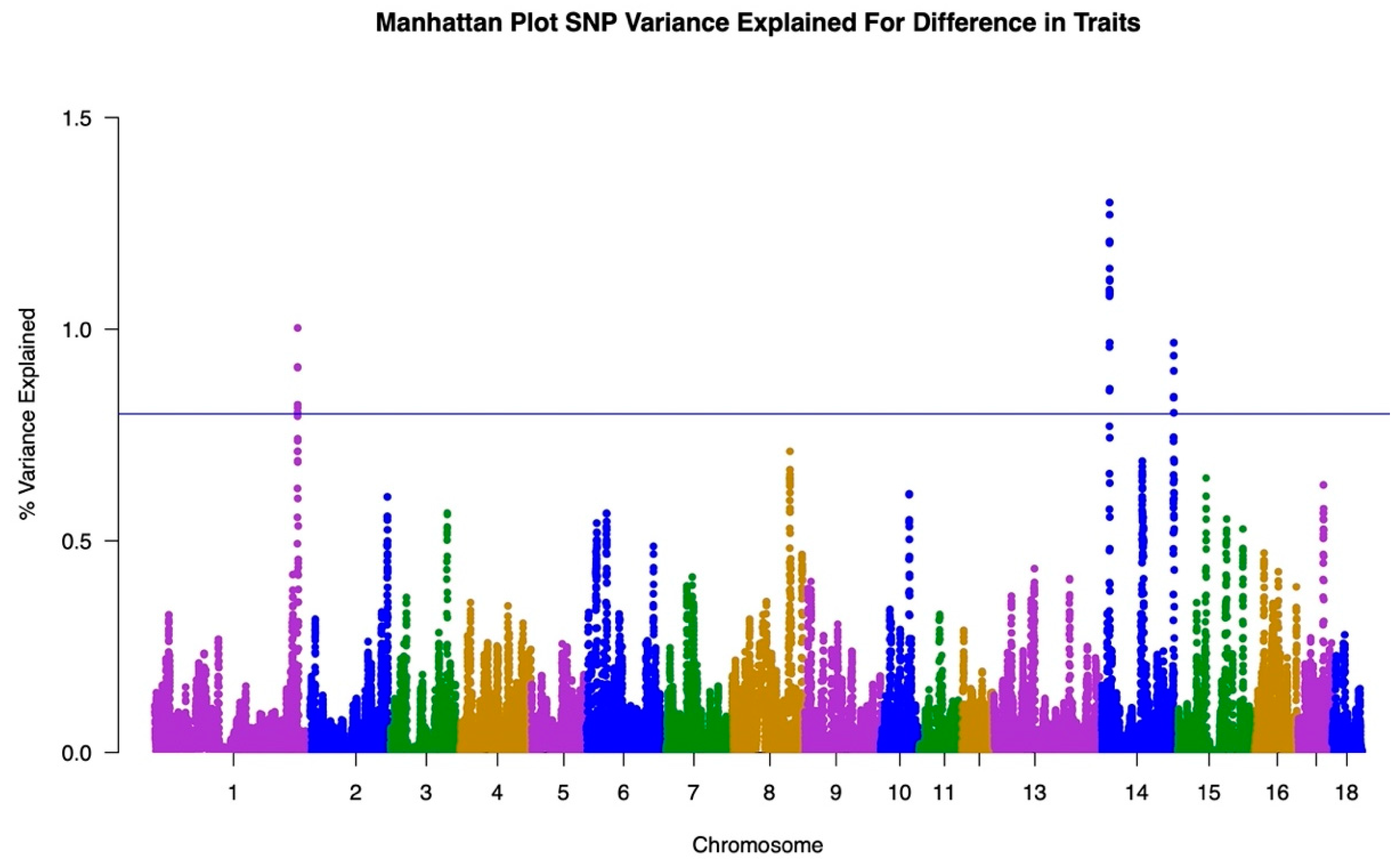
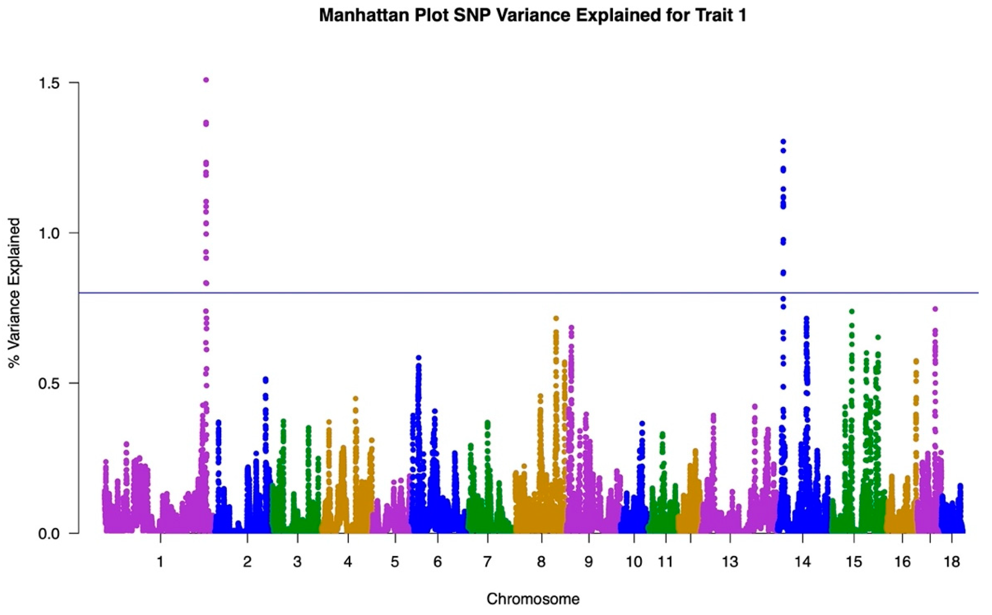
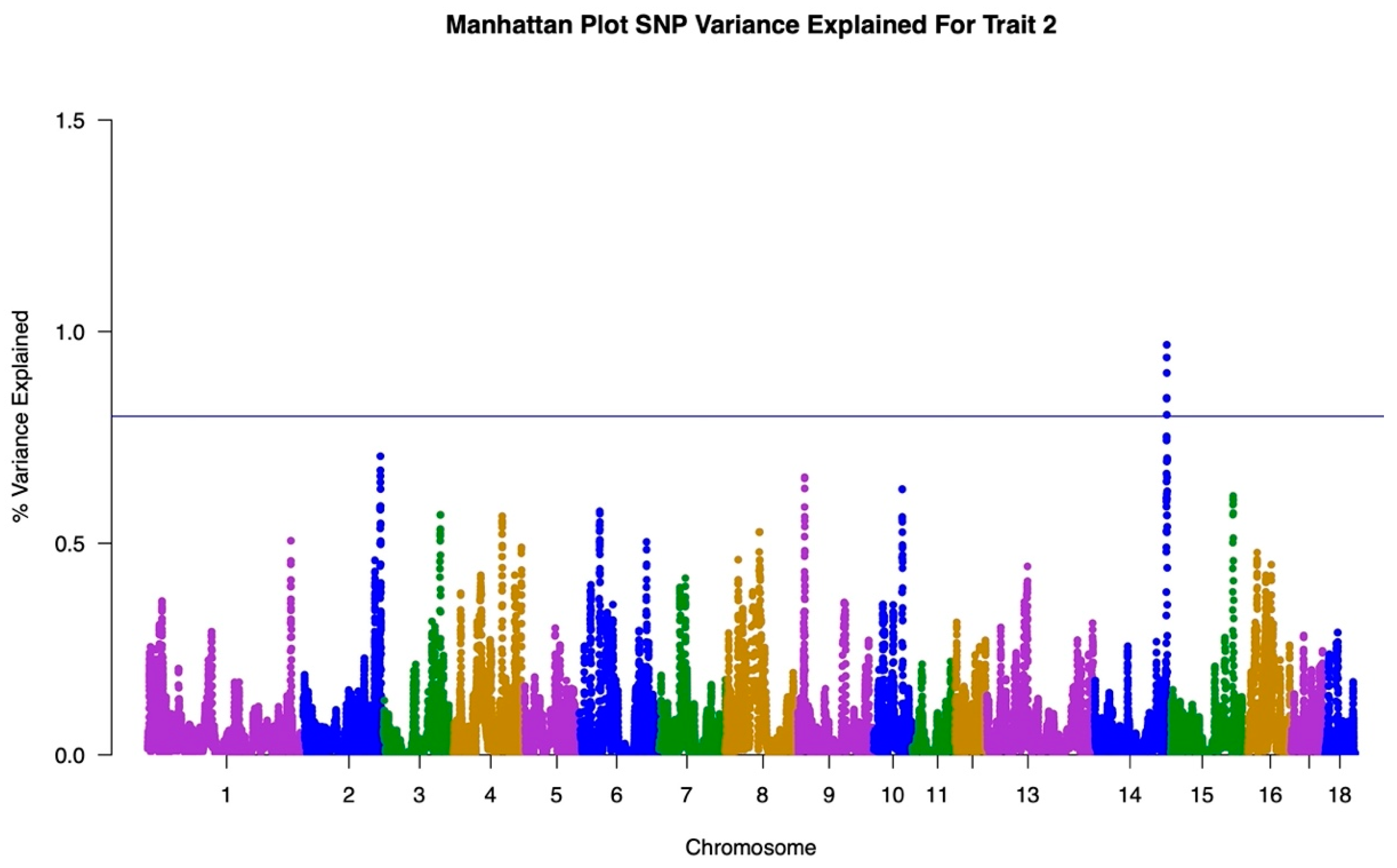
3.1. GWAS
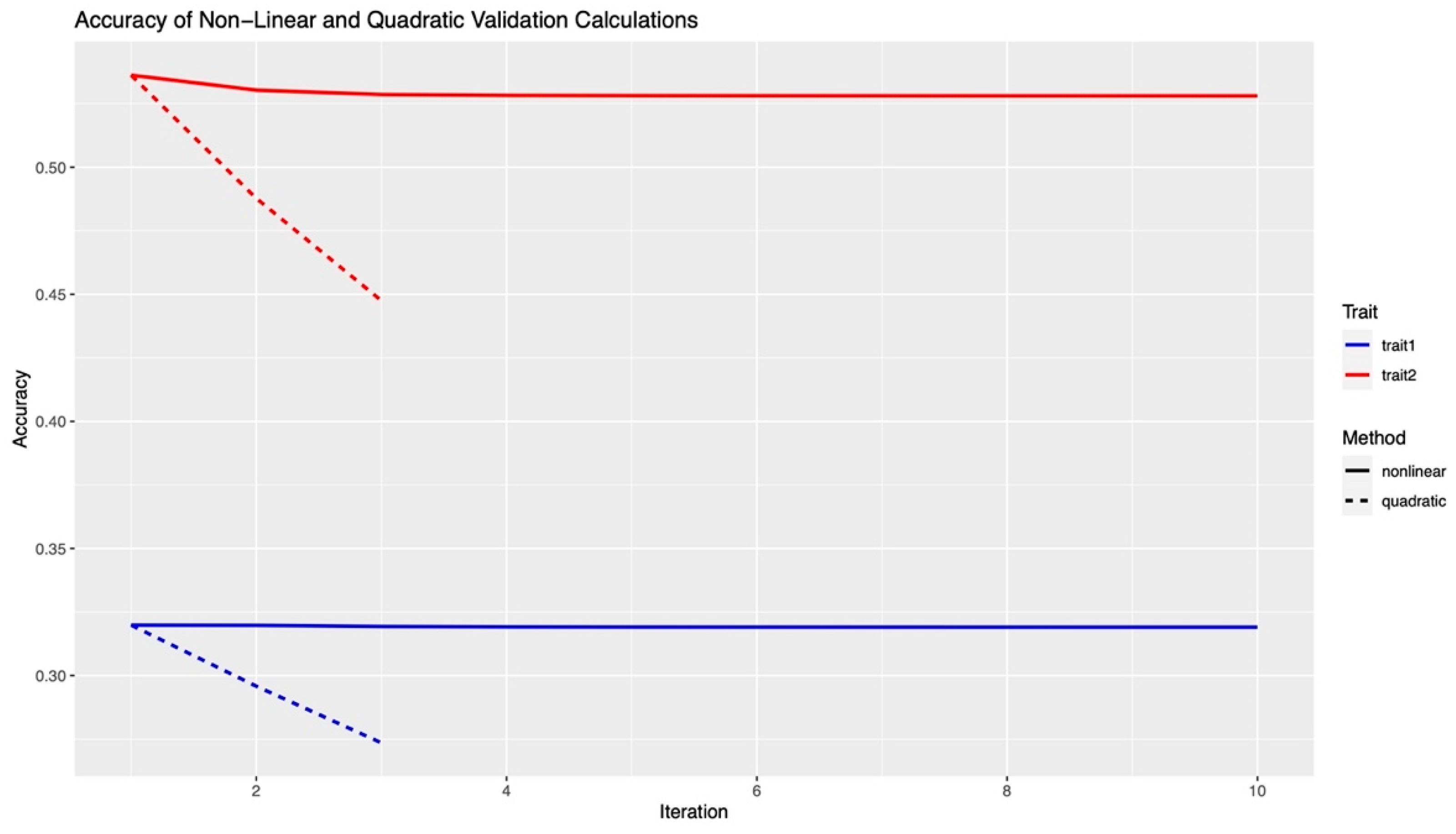
3.2. Validation and Accuracy
4. Discussion
5. Conclusions
Author Contributions
Funding
Institutional Review Board Statement
Informed Consent Statement
Data Availability Statement
Acknowledgments
Conflicts of Interest
References
- Oliveira, R.F.; Moreira, R.H.R.; Abreu, M.L.T.; Gionbelli, M.P.; Teixeira, A.O.; Cantarelli, V.S. Effects of air temperature on physiology and productive performance of pigs during growing and finishing phases. S. Afr. J. Anim. Sci. 2018, 48, 627–635. Available online: http://www.scielo.org.za/scielo.php?script=sci_abstract&pid=S0375-15892018000400004&lng=en&nrm=iso&tlng=en (accessed on 31 October 2021). [CrossRef]
- St-Pierre, N.; Cobanov, B.; Schnitkey, G. Economic Losses from Heat Stress by US Livestock Industries. J. Dairy Sci. 2003, 86, E52–E77. Available online: https://www.sciencedirect.com/science/article/pii/S0022030203740405 (accessed on 31 October 2021). [CrossRef] [Green Version]
- Fragomeni, B.O.; Lourenco, D.A.L.; Tsuruta, S.; Andonov, S.; Gray, K.; Huang, Y.; Misztal, I. Modeling response to heat stress in pigs from nucleus and commercial farms in different locations in the United States. J. Anim. Sci. 2016, 94, 4789–4798. Available online: https://academic.oup.com/jas/article/94/11/4789/4703038 (accessed on 30 November 2021). [CrossRef] [PubMed]
- Knap, P.W. Pig Breedingpigbreedingfor Increased Sustainability. In Encyclopedia of Sustainability Science and Technology; Meyers, R.A., Ed.; Springer: New York, NY, USA, 2012; pp. 7972–8012. [Google Scholar] [CrossRef]
- Zumbach, B.; Misztal, I.; Tsuruta, S.; Sanchez, J.P.; Azain, M.; Herring, W.; Holl, J.; Long, T.; Culbertson, M. Genetic components of heat stress in finishing pigs: Parameter estimation. J. Anim. Sci. 2008, 86, 2076–2081. [Google Scholar] [CrossRef] [Green Version]
- Fragomeni, B.O.; Lourenco, D.A.L.; Tsuruta, S.; Bradford, H.L.; Gray, K.A.; Huang, Y.; Misztal, I. Using single-step genomic best linear unbiased predictor to enhance the mitigation of seasonal losses due to heat stress in pigs. J. Anim. Sci. 2016, 94, 5004–5013. [Google Scholar] [CrossRef] [Green Version]
- Aguilar, I.; Misztal, I.; Johnson, D.L.; Legarra, A.; Tsuruta, S.; Lawlor, T.J. Hot topic: A unified approach to utilize phenotypic, full pedigree, and genomic information for genetic evaluation of Holstein final score1. J. Dairy Sci. 2010, 93, 743–752. Available online: https://www.sciencedirect.com/science/article/pii/S0022030210715174 (accessed on 31 October 2021). [CrossRef]
- Christensen, O.F.; Lund, M.S. Genomic prediction when some animals are not genotyped. Genet. Sel. Evol. 2010, 42, 2. [Google Scholar] [CrossRef] [Green Version]
- Misztal, I. Studies on Inflation of GEBV in Single-Step GBLUP for Type. Interbull Bull. 2017. Available online: https://journal.interbull.org/index.php/ib/article/view/1425 (accessed on 31 October 2021).
- Schaeffer, L.R. Strategy for applying genome-wide selection in dairy cattle. J. Anim. Breed. Genet. 2006, 123, 218–223. Available online: http://onlinelibrary.wiley.com/doi/abs/10.1111/j.1439-0388.2006.00595.x (accessed on 30 November 2021). [CrossRef]
- Aguilar, I.; Legarra, A.; Cardoso, F.; Masuda, Y.; Lourenco, D.; Misztal, I. Frequentist p-values for large-scale-single step genome-wide association, with an application to birth weight in American Angus cattle. Genet. Sel. Evol. 2019, 51, 28. [Google Scholar] [CrossRef] [Green Version]
- Wang, H.; Misztal, I.; Aguilar, I.; Legarra, A.; Muir, W.M. Genome-wide association mapping including phenotypes from relatives without genotypes. Genet. Res. 2012, 94, 73–83. [Google Scholar] [CrossRef] [Green Version]
- Zhang, X.; Lourenco, D.; Aguilar, I.; Legarra, A.; Misztal, I. Weighting Strategies for Single-Step Genomic BLUP: An Iterative Approach for Accurate Calculation of GEBV and GWAS. Front. Genet. 2016, 7, 151. Available online: https://www.frontiersin.org/article/10.3389/fgene.2016.00151 (accessed on 31 October 2021). [CrossRef] [PubMed] [Green Version]
- Narasimhan, R. Weather Data: Get Weather Data from the Web. R Package. 2014. Available online: https://cran.r-project.org/package=weatherData (accessed on 31 October 2021).
- Legarra, A.; Aguilar, I.; Misztal, I. A relationship matrix including full pedigree and genomic information. J. Dairy Sci. 2009, 92, 4656–4663. [Google Scholar] [CrossRef] [PubMed] [Green Version]
- VanRaden, P.M. Efficient methods to compute genomic predictions. J. Dairy Sci. 2008, 91, 4414–4423. [Google Scholar] [CrossRef] [Green Version]
- Zhang, Z.; Liu, J.; Ding, X.; Bijma, P.; de Koning, D.-J.; Zhang, Q. Best Linear Unbiased Prediction of Genomic Breeding Values Using a Trait-Specific Marker-Derived Relationship Matrix. PLoS ONE 2010, 5, e12648. Available online: https://journals.plos.org/plosone/article?id=10.1371/journal.pone.0012648 (accessed on 12 November 2021). [CrossRef] [Green Version]
- Cole, J.B.; VanRaden, P.M.; O’Connell, J.R.; Van Tassell, C.P.; Sonstegard, T.S.; Schnabel, R.D.; Taylor, J.F.; Wiggans, G.R. Distribution and location of genetic effects for dairy traits. J. Dairy Sci. 2009, 92, 2931–2946. Available online: https://www.sciencedirect.com/science/article/pii/S0022030209706095 (accessed on 31 October 2021). [CrossRef] [PubMed] [Green Version]
- Legarra, A.; Reverter, A. Semi-parametric estimates of population accuracy and bias of predictions of breeding values and future phenotypes using the LR method. Genet. Sel. Evol. 2018, 50, 53. [Google Scholar] [CrossRef] [PubMed] [Green Version]
- Misztal, I.; Tsuruta, S.; Strabel, T.; Auvray, B.; Druet, T.; Lee, D.H. Blupf90 and Related Programs (BGF90). In Proceedings of the 7th World Congress on Genetics Applied to Livestock Production, Montpellier, France, 19–32 August 2002. [Google Scholar]
- Aguilar, I.; Misztal, I.; Tsuruta, S.; Legarra, A.; Wang, H. PREGSF90–POSTGSF90: Computational Tools for the Implementation of Single-step Genomic Selection and Genome-wide Association with Ungenotyped Individuals in BLUPF90 Programs. In Proceedings of the 10th World Congress on Genetics Applied to Livestock Production, Vancouver, BC, Canada, 17–22 August 2014. [Google Scholar]
- Fonseca, P.A.; Suárez-Vega, A.; Marras, G.; Cánovas, Á. GALLO: An R package for genomic annotation and integration of multiple data sources in livestock for positional candidate loci. GigaScience 2020, 9, giaa149. Available online: https://academic.oup.com/gigascience/article/doi/10.1093/gigascience/giaa149/6055471 (accessed on 10 November 2021). [CrossRef]
- Hu, Z.-L.; Park, C.A.; Wu, X.-L.; Reecy, J.M. Animal QTLdb: An improved database tool for livestock animal QTL/association data dissemination in the post-genome era. Nucleic Acids Res. 2012, 41, D871–D879. Available online: http://academic.oup.com/nar/article/41/D1/D871/1063071/Animal-QTLdb-an-improved-database-tool-for (accessed on 1 December 2021). [CrossRef] [Green Version]
- Usala, M.; Macciotta, N.P.P.; Bergamaschi, M.; Maltecca, C.; Fix, J.; Schwab, C.; Shull, C.; Tiezzi, F. Genetic Parameters for Tolerance to Heat Stress in Crossbred Swine Carcass Traits. Front. Genet. 2021, 11, 1821. Available online: https://www.frontiersin.org/article/10.3389/fgene.2020.612815 (accessed on 31 October 2021). [CrossRef]
- Mulder, H.A.; Bijma, P. Effects of genotype x environment interaction on genetic gain in breeding programs. J. Anim. Sci. 2005, 83, 49–61. [Google Scholar] [CrossRef]
- Robertson, A. The Sampling Variance of the Genetic Correlation Coefficient. Biometrics 1959, 15, 469. Available online: https://www.jstor.org/stable/2527750 (accessed on 31 October 2021). [CrossRef]
- Mulder, H.; Veerkamp, R.; Ducro, B.; van Arendonk, J.; Bijma, P. Optimization of Dairy Cattle Breeding Programs for Different Environments with Genotype by Environment Interaction. J. Dairy Sci. 2006, 89, 1740–1752. Available online: https://www.sciencedirect.com/science/article/pii/S0022030206722421 (accessed on 31 October 2021). [CrossRef] [Green Version]
- Dikmen, S.; Cole, J.B.; Null, D.J.; Hansen, P.J. Genome-Wide Association Mapping for Identification of Quantitative Trait Loci for Rectal Temperature during Heat Stress in Holstein Cattle. Moore, S., editor. PLoS ONE 2013, 8, e69202. Available online: https://dx.plos.org/10.1371/journal.pone.0069202 (accessed on 31 October 2021). [CrossRef] [PubMed] [Green Version]
- Otto, P.I.; Guimarães, S.E.; Verardo, L.L.; Azevedo, A.L.S.; Vandenplas, J.; Sevillano, C.A.; Marques, D.B.; Pires, M.D.F.A.; de Freitas, C.; Verneque, R.S.; et al. Genome-wide association studies for heat stress response in Bos taurus × Bos indicus crossbred cattle. J. Dairy Sci. 2019, 102, 8148–8158. [Google Scholar] [CrossRef] [Green Version]
- Lourenco, D.A.L.; Fragomeni, B.O.; Bradford, H.L.; Menezes, I.R.; Ferraz, J.B.S.; Aguilar, I.; Tsuruta, S.; Misztal, I. Implications of SNP weighting on single-step genomic predictions for different reference population sizes. J. Anim. Breed Genet. Z. Tierz. Zucht. 2017, 134, 463–471. [Google Scholar] [CrossRef]
- Goddard, M. Genomic selection: Prediction of accuracy and maximisation of long term response. Genetica 2009, 136, 245–257. [Google Scholar] [CrossRef]
- Daetwyler, H.D.; Pong-Wong, R.; Villanueva, B.; Woolliams, J.A. The impact of genetic architecture on genome-wide evaluation methods. Genetics 2010, 185, 1021–1031. [Google Scholar] [CrossRef] [Green Version]
- Uimari, P.; Tapio, M. Extent of linkage disequilibrium and effective population size in Finnish Landrace and Finnish Yorkshire pig breeds. J. Anim. Sci. 2011, 89, 609–614. [Google Scholar] [CrossRef]
- Rohrer, G.A.; Alexander, L.J.; Hu, Z.; Smith, T.P.; Keele, J.W.; Beattie, C.W. A comprehensive map of the porcine genome. Genome Res. 1996, 6, 371–391. [Google Scholar] [CrossRef] [Green Version]
- Misztal, I.; Legarra, A.; Aguilar, I. Using recursion to compute the inverse of the genomic relationship matrix. J. Dairy Sci. 2014, 97, 3943–3952. [Google Scholar] [CrossRef]
- Fragomeni, B.; Lourenco, D.; Tsuruta, S.; Masuda, Y.; Aguilar, I.; Misztal, I. Use of genomic recursions and algorithm for proven and young animals for single-step genomic BLUP analyses—A simulation study. J. Anim. Breed Genet. Z. Tierz. Zucht. 2015, 132, 340–345. [Google Scholar] [CrossRef] [PubMed]
- Fragomeni, B.O.; Lourenco, D.A.L.; Tsuruta, S.; Masuda, Y.; Aguilar, I.; Legarra, A.; Lawlor, T.J.; Misztal, I. Hot topic: Use of genomic recursions in single-step genomic best linear unbiased predictor (BLUP) with a large number of genotypes. J. Dairy Sci. 2015, 98, 4090–4094. Available online: https://www.sciencedirect.com/science/article/pii/S0022030215002386 (accessed on 30 November 2021). [CrossRef] [PubMed] [Green Version]
- Pocrnic, I.; Lourenco, D.A.L.; Masuda, Y.; Legarra, A.; Misztal, I. The Dimensionality of Genomic Information and Its Effect on Genomic Prediction. Genetics 2016, 203, 573–581. Available online: https://www.genetics.org/content/203/1/573 (accessed on 31 October 2021). [CrossRef]
- Fragomeni, B.D.O.; Misztal, I.; Lourenco, D.L.; Aguilar, I.; Okimoto, R.; Muir, W.M. Changes in variance explained by top SNP windows over generations for three traits in broiler chicken. Front. Genet. 2014, 5, 332. Available online: https://www.frontiersin.org/article/10.3389/fgene.2014.00332 (accessed on 31 October 2021). [CrossRef] [PubMed] [Green Version]
- Hossain, D.; Shih, S.Y.-P.; Xiao, X.; White, J.; Tsang, W.Y. Cep44 functions in centrosome cohesion by stabilizing rootletin. J. Cell Sci. 2020, 133, jcs.239616. Available online: https://journals.biologists.com/jcs/article/doi/10.1242/jcs.239616/266270/Cep44-functions-in-centrosome-cohesion-by (accessed on 31 October 2021).
- FBXO8 F-Box Protein 8 [Homo Sapiens (Human)]-Gene-NCBI. Available online: https://www.ncbi.nlm.nih.gov/gene/26269 (accessed on 31 October 2021).
- HPGD 15-Hydroxyprostaglandin Dehydrogenase [Homo Sapiens (Human)]-Gene-NCBI. Available online: https://www.ncbi.nlm.nih.gov/gene/3248 (accessed on 7 December 2021).
- GLRA3 Glycine Receptor Alpha 3 [Homo Sapiens (Human)]-Gene-NCBI. Available online: https://www.ncbi.nlm.nih.gov/gene/8001 (accessed on 7 December 2021).
- TGFBR1 Transforming Growth Factor Beta Receptor 1 [Homo Sapiens (Human)]-Gene-NCBI. Available online: https://www.ncbi.nlm.nih.gov/gene/7046 (accessed on 31 October 2021).
- Waide, E.H.; Tuggle, C.K.; Serão, N.V.L.; Schroyen, M.; Hess, A.; Rowland, R.R.R.; Lunney, J.K.; Plastow, G.; Dekkers, J.C.M. Genomewide association of piglet responses to infection with one of two porcine reproductive and respiratory syndrome virus isolates. J. Anim. Sci. 2017, 95, 16–38. [Google Scholar] [CrossRef]
- Jiao, S.; Maltecca, C.; Gray, K.A.; Cassady, J.P. Feed intake, average daily gain, feed efficiency, and real-time ultrasound traits in Duroc pigs: II. Genomewide association. J. Anim. Sci. 2014, 92, 2846–2860. [Google Scholar] [CrossRef]
- Patience, J.F.; Rossoni-Serão, M.C.; Gutiérrez, N.A. A review of feed efficiency in swine: Biology and application. J. Anim. Sci. Biotechnol. 2015, 6, 33. Available online: https://www.ncbi.nlm.nih.gov/pmc/articles/PMC4527244/ (accessed on 31 October 2021). [CrossRef] [PubMed] [Green Version]
- Apple, J. Nutritional effects on pork quality in swine production. Natl. Swine Nutr. Guide 2010. PIG 12-02-02:288–299. [Google Scholar]
- Lammers, P.; Stender, D.; Honeyman, M. Nutritional Effects on Pork Quality in Swine Production. In Niche Pork Production; Iowa State University Animal Industry Report; Iowa State University Digital Press: Ames, IA, USA, 2007. [Google Scholar] [CrossRef] [Green Version]


| Item | Trait One: Under Heat Stress | Trait Two: No Heat Stress | Total |
|---|---|---|---|
| No. | 32,783 | 194,260 | 227,043 |
| Weight, kg | 89.9 | 94.2 | 93.2 |
| Age, d | 188.10 | 184.87 | 185.30 |
| North Carolina, no. | 29,296 | 111,319 | 140,615 |
| Missouri, no. | 3487 | 82,941 | 86,428 |
| Result | Trait One: Under Heat Stress | Trait Two: No Heat Stress |
|---|---|---|
| Random Residual Variance Component | 216.69 | 210.69 |
| Litter Variance Component | 31.736 | 30.791 |
| Genetic Variance Component | 84.697 | 60.173 |
| Heritability | 0.25 | 0.20 |
| Genetic Correlation | 0.63 | |
Publisher’s Note: MDPI stays neutral with regard to jurisdictional claims in published maps and institutional affiliations. |
© 2022 by the authors. Licensee MDPI, Basel, Switzerland. This article is an open access article distributed under the terms and conditions of the Creative Commons Attribution (CC BY) license (https://creativecommons.org/licenses/by/4.0/).
Share and Cite
Dodd, G.R.; Gray, K.; Huang, Y.; Fragomeni, B. Single-Step GBLUP and GWAS Analyses Suggests Implementation of Unweighted Two Trait Approach for Heat Stress in Swine. Animals 2022, 12, 388. https://doi.org/10.3390/ani12030388
Dodd GR, Gray K, Huang Y, Fragomeni B. Single-Step GBLUP and GWAS Analyses Suggests Implementation of Unweighted Two Trait Approach for Heat Stress in Swine. Animals. 2022; 12(3):388. https://doi.org/10.3390/ani12030388
Chicago/Turabian StyleDodd, Gabriella Roby, Kent Gray, Yijian Huang, and Breno Fragomeni. 2022. "Single-Step GBLUP and GWAS Analyses Suggests Implementation of Unweighted Two Trait Approach for Heat Stress in Swine" Animals 12, no. 3: 388. https://doi.org/10.3390/ani12030388
APA StyleDodd, G. R., Gray, K., Huang, Y., & Fragomeni, B. (2022). Single-Step GBLUP and GWAS Analyses Suggests Implementation of Unweighted Two Trait Approach for Heat Stress in Swine. Animals, 12(3), 388. https://doi.org/10.3390/ani12030388