
The Effect of Rider:Horse Bodyweight Ratio on the Superficial Body Temperature of Horse’s Thoracolumbar Region Evaluated by Advanced Thermal Image Processing

 , , , , , and
Abstract
:Simple Summary
Abstract
1. Introduction
2. Materials and Methods
2.1. Animals
2.2. Riders
2.3. Standardized Exercise Test and Thermal Images Acquisition
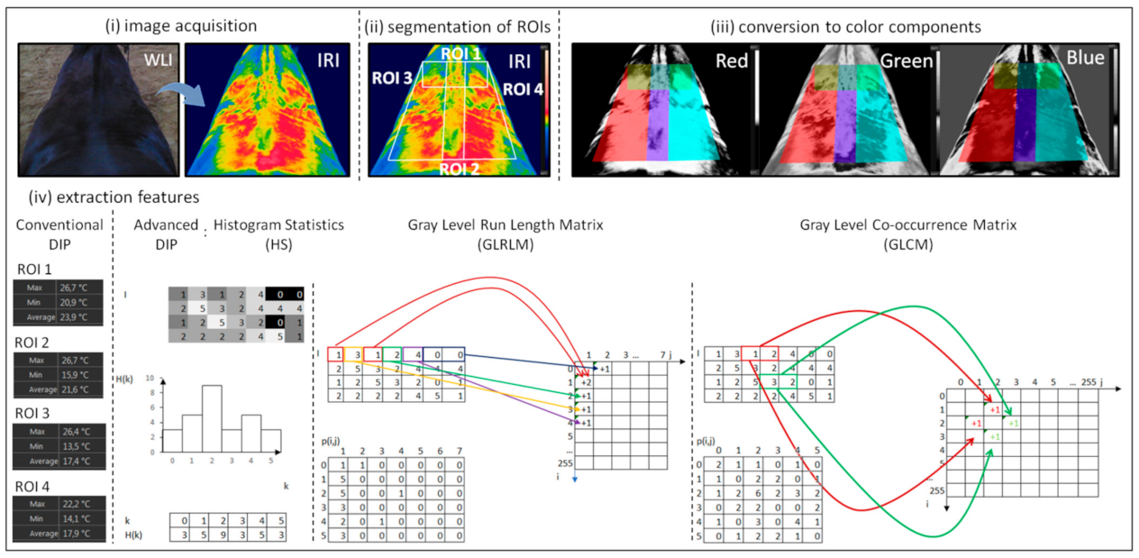
2.4. Digital Image Processing
2.4.1. Conventional Digital Image Processing
2.4.2. Advanced Digital Image Processing
2.5. Data Analysis
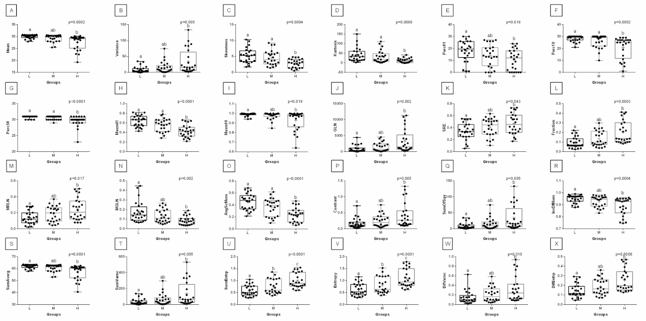
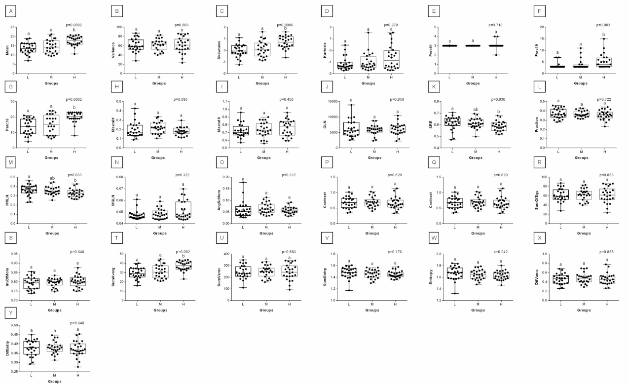
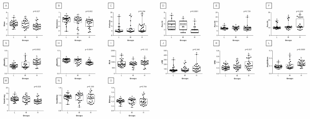
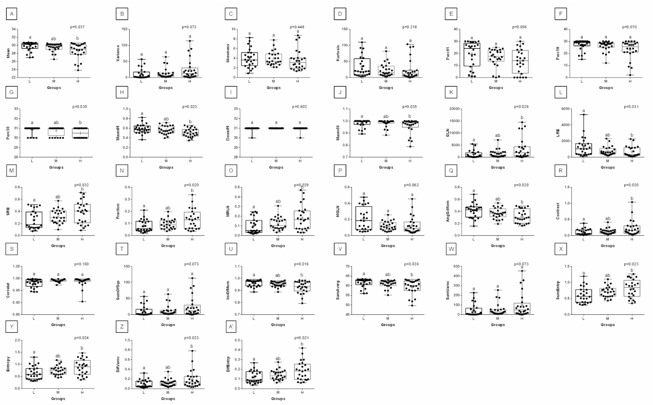
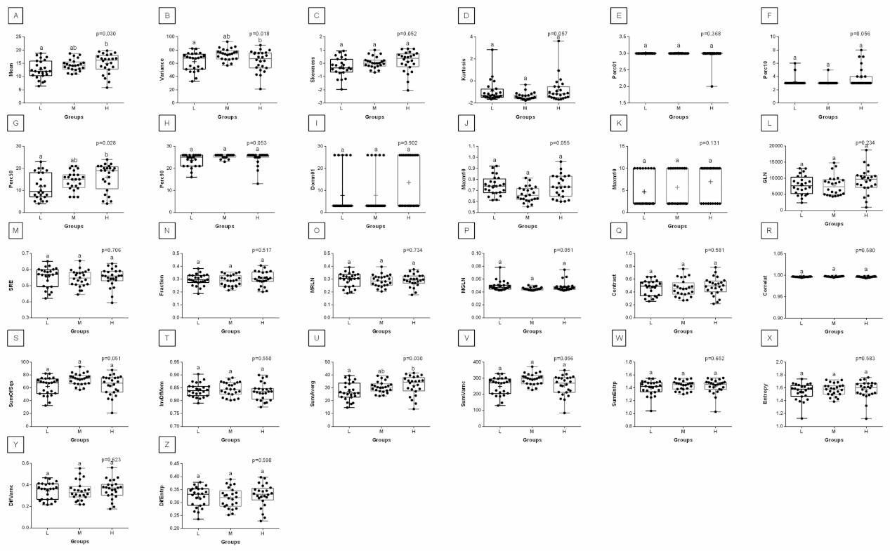
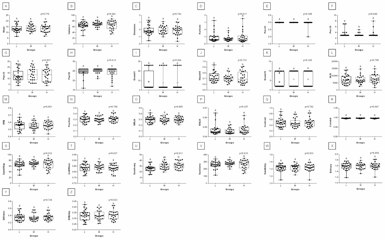
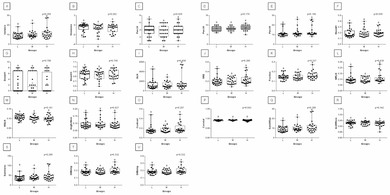
3. Results
4. Discussion
5. Conclusions
Supplementary Materials
Author Contributions
Funding
Institutional Review Board Statement
Data Availability Statement
Conflicts of Interest
References
- Han, J.; Lawler, D.; Kimm, S. Childhood obesity. Lancet 2015, 375, 1737–1748. [Google Scholar] [CrossRef]
- Wang, Y.; McPherson, K.; March, T.; Gortmaker, S.; Brown, M. Health and economic burden of the projected obesity trends in the USA and UK. Lancet 2017, 378, 815–825. [Google Scholar] [CrossRef]
- Forino, S.; Cameron, L.; Stones, N.; Freeman, M. Potential Impacts of Body Image Perception in Female Equestrians. J. Equine Vet. Sci. 2021, 107, 103776. [Google Scholar] [CrossRef]
- Kozak, M.W. Making trails: Horses and equestrian tourism in Poland. In Equestrian Cultures in Global and Local Contexts; Springer: Cham, Switzerland, 2017; pp. 131–152. [Google Scholar]
- Matsuura, A.; Mano, H.; Irimajiri, M.; Hodate, K. Maximum permissible load for Yonaguni ponies (Japanese landrace horses) trotting over a short, straight course. Anim. Welf. 2016, 25, 151–156. [Google Scholar] [CrossRef]
- Garlinghouse, S.; Burill, M. Relationship of body condition score to completion rate during 160 km endurance races. Equine Vet. J. 1999, 31 (Suppl. S30), 591–595. [Google Scholar] [CrossRef] [PubMed]
- Matsuura, A.; Sakuma, S.; Irimajiri, M.; Hodate, K. Maximum permissible load weight of a Taishuh pony at a trot. J. Anim. Sci. 2013, 91, 3989–3996. [Google Scholar] [CrossRef]
- Clayton, H.; Dyson, S.; Harris, P.; Bondi, A. Horses, saddles and riders: Applying the science. Equine Vet. Educ. 2015, 27, 447–452. [Google Scholar] [CrossRef]
- Hall, C.; Kay, R.; Randle, H.; Preshaw, L.; Pearson, G.; Waran, N. Indicators on the outside: Behaviour and equine quality of life. In Proceedings of the 15th International Conference of the International Society for Equitation Science, Guelph, ON, Canada, 19–21 August 2019. [Google Scholar]
- Randle, H.; Henshall, C.; Hall, C.; Pearson, G.; Preshaw, L.; Waran, N. Indicators on the inside: Physiology and equine quality of life. In Proceedings of the 15th International Conference of the International Society for Equitation Science, Guelph, ON, Canada, 19–21 August 2019. [Google Scholar]
- Hall, C.; Randle, H.; Pearson, G.; Preshaw, L.; Waran, N. Assessing equine emotional state. Appl. Anim. Behav. Sci. 2018, 205, 183–193. [Google Scholar] [CrossRef] [Green Version]
- Becker-Birck, M.; Schmidt, A.; Lasarzik, J.; Aurich, J.; Möstl, E.; Aurich, C. Cortisol release and heart rate variability in sport horses participating in equestrian competitions. J. Vet. Behav. 2013, 8, 87–94. [Google Scholar] [CrossRef]
- Waran, N.K.; Cuddeford, D. Effects of loading and transport on the heart rate and behaviour of horses. Appl. Anim. Behav. Sci. 1995, 43, 71–81. [Google Scholar] [CrossRef]
- Thayer, J.F.; Sternberg, E. Beyond heart rate variability: Vagal regulation of allostatic systems. Ann. N. Y. Acad. Sci. 2006, 1088, 361–372. [Google Scholar] [CrossRef] [PubMed]
- Visser, E.K.; Van Reenen, C.G.; Van der Werf, J.T.N.; Schilder, M.B.H.; Knaap, J.H.; Barneveld, A.; Blokhuis, H.J. Heart rate and heart rate variability during a novel object test and a handling test in young horses. Physiol. Behav. 2002, 76, 289–296. [Google Scholar] [CrossRef]
- Waran, N.; Randle, H. What we can measure, we can manage: The importance of using robust welfare indicators in Equitation Science. Appl. Anim. Behav. Sci. 2017, 190, 74–81. [Google Scholar] [CrossRef]
- de Mira, M.C.; Lamy, E.; Santos, R.; Williams, J.; Pinto, M.V.; Martins, P.S.; Rodrigues, P.; Marlin, D. Salivary cortisol and eye temperature changes during endurance competitions. BMC Vet. Res. 2021, 17, 329. [Google Scholar] [CrossRef] [PubMed]
- Hall, C.; Burton, K.; Maycock, E.; Wragg, E. A preliminary study into the use of infrared thermography as a means of assessing the horse’s response to different training methods. J. Vet. Behav. 2011, 6, 291–292. [Google Scholar] [CrossRef] [Green Version]
- Redaelli, V.; Luzi, F.; Mazzola, S.; Bariffi, G.D.; Zappaterra, M.; Nanni Costa, L.; Padalino, B. The use of infrared thermography (IRT) as stress indicator in horses trained for endurance: A pilot study. Animals 2019, 9, 84. [Google Scholar] [CrossRef] [Green Version]
- Travain, T.; Valsecchi, P. Infrared Thermography in the Study of Animals’ Emotional Responses: A Critical Review. Animals 2021, 11, 2510. [Google Scholar] [CrossRef]
- Soroko, M.; Howell, K. Infrared thermography: Current applications in equine medicine. J. Equine Vet. Sci. 2018, 60, 90–96. [Google Scholar] [CrossRef]
- Roberto, J.V.B.; De Souza, B.B. Use of infrared thermography in veterinary medicine and animal production. J. Anim. Behav. Biometeorol. 2020, 2, 73–84. [Google Scholar] [CrossRef]
- Witkowska-Piłaszewicz, O.; Maśko, M.; Domino, M.; Winnicka, A. Infrared thermography correlates with lactate concentration in blood during race training in horses. Animals 2020, 10, 2072. [Google Scholar] [CrossRef]
- Wilk, I.; Wnuk-Pawlak, E.; Janczarek, I.; Kaczmarek, B.; Dybczyńska, M.; Przetacznik, M. Distribution of superficial body temperature in horses ridden by two riders with varied body weights. Animals 2020, 10, 340. [Google Scholar] [CrossRef] [PubMed] [Green Version]
- Masko, M.; Borowska, M.; Domino, M.; Jasinski, T.; Zdrojkowski, L.; Gajewski, Z. A novel approach to thermographic images analysis of equine thoracolumbar region: The effect of effort and rider’s body weight on structural image complexity. BMC Vet. Res. 2021, 17, 99. [Google Scholar] [CrossRef]
- Powell, D.; Bennett-Wimbush, K.; Peeples, A.; Duthie, M. Evaluation of indicators of weight-carrying ability of light riding horses. J. Equine Vet. Sci. 2008, 28, 28–33. [Google Scholar] [CrossRef]
- Christensen, J.W.; Bathellier, S.; Rhodin, M.; Palme, R.; Uldahl, M. Increased rider weight did not induce changes in behavior and physiological parameters in horses. Animals 2020, 10, 95. [Google Scholar] [CrossRef] [PubMed] [Green Version]
- Christensen, J.W.; Beekmans, M.; van Dalum, M.; Van Dierendonck, M. Effects of hyperflexion on acute stress responses in ridden dressage horses. Physiol. Behav. 2014, 128, 39–45. [Google Scholar] [CrossRef]
- Zebisch, A.; May, A.; Reese, S.; Gehlen, H. Effect of different head-neck positions on physical and psychological stress parameters in the ridden horse. J. Anim. Physiol. Anim. Nutr. 2014, 98, 901–907. [Google Scholar] [CrossRef] [PubMed]
- Dyson, S.; Ellis, A.D.; Mackechnie-Guire, R.; Douglas, J.; Bondi, A.; Harris, P. The influence of rider:horse bodyweight ratio and rider-horse-saddle fit on equine gait and behaviour: A pilot study. Equine Vet. Educ. 2020, 32, 527–539. [Google Scholar] [CrossRef] [Green Version]
- Resmini, R.; Silva, L.; Araujo, A.S.; Medeiros, P.; Muchaluat-Saade, D.; Conci, A. Combining Genetic Algorithms and SVM for Breast Cancer Diagnosis Using Infrared Thermography. Sensors 2021, 21, 4802. [Google Scholar] [CrossRef]
- Depeursinge, A.; Al-Kadi, O.S.; Mitchell, J.R. Biomedical Texture Analysis: Fundamentals, Tools and Challenges; Academic Press: Cambridge, MA, USA, 2017. [Google Scholar]
- Bębas, E.; Borowska, M.; Derlatka, M.; Oczeretko, E.; Hładuński, M.; Szumowski, P.; Mojsak, M. Machine-learning-based classification of the histological subtype of non-small-cell lung cancer using MRI texture analysis. Biomed. Signal Process. Control 2021, 66, 102446. [Google Scholar] [CrossRef]
- Sohail, A.S.M.; Bhattacharya, P.; Mudur, S.P.; Krishnamurthy, S. Local relative GLRLM-based texture feature extraction for classifying ultrasound medical images. In Proceedings of the 2011 24th Canadian Conference on Electrical and Computer Engineering (CCECE, IEEE), Niagara Falls, ON, Canada, 8–11 May 2011; pp. 1092–1095. [Google Scholar]
- Girejko, G.; Borowska, M.; Szarmach, J. Statistical analysis of radiographic textures illustrating healing process after the guided bone regeneration surgery. In International Conference on Information Technologies in Biomedicine; Springer: Cham, Switzerland, 2018; pp. 217–226. [Google Scholar]
- Obuchowicz, R.; Nurzynska, K.; Obuchowicz, B.; Urbanik, A.; Piórkowski, A. Caries detection enhancement using texture feature maps of intraoral radiographs. Oral Radiol. 2020, 36, 275–287. [Google Scholar] [CrossRef] [Green Version]
- Pociask, E.; Nurzynska, K.; Obuchowicz, R.; Bałon, P.; Uryga, D.; Strzelecki, M.; Izworski, A.; Piórkowski, A. Differential Diagnosis of Cysts and Granulomas Supported by Texture Analysis of Intraoral Radiographs. Sensors 2021, 21, 7481. [Google Scholar] [CrossRef]
- Zhang, H.; Hung, C.L.; Min, G.; Guo, J.P.; Liu, M.; Hu, X. GPU-accelerated GLRLM algorithm for feature extraction of MRI. Sci. Rep. 2019, 9, 10883. [Google Scholar] [CrossRef]
- Domino, M.; Borowska, M.; Kozłowska, N.; Zdrojkowski, Ł.; Jasiński, T.; Smyth, G.; Maśko, M. Advances in Thermal Image Analysis for the Detection of Pregnancy in Horses Using Infrared Thermography. Sensors 2022, 22, 191. [Google Scholar] [CrossRef]
- Silva, T.A.E.; Silva, L.F.; Muchaluat-Saade, D.C.; Conci, A. A computational method to assist the diagnosis of breast disease using dynamic thermography. Sensors 2020, 20, 3866. [Google Scholar] [CrossRef] [PubMed]
- Martin, B.B., Jr.; Klide, A.M. Physical examination of horses with back pain. Vet. Clin. N. Am. Equine Pract. 1999, 15, 61–70. [Google Scholar] [CrossRef]
- Dyson, S. Can lameness be reliably graded? Equine Vet. J. 2011, 43, 379–382. [Google Scholar] [CrossRef] [PubMed]
- Greve, L.; Dyson, S. Saddle fit and management: An investigation of the association with equine thoracolumbar asymmetries, horse and rider health. Equine Vet. J. 2015, 47, 415–421. [Google Scholar] [CrossRef] [PubMed]
- Williams, J.; Tabor, G. Rider impacts on equitation. Appl. Anim. Behav. Sci. 2017, 190, 28–42. [Google Scholar] [CrossRef]
- NIH. Calculate Your Body Mass Index. 2018. Available online: https://www.nhlbi.nih.gov/health/educational/lose_wt/BMI/bmicalc.htm (accessed on 10 April 2021).
- McCafferty, D.J. The value of infrared thermography for research on mammals: Previous applications and future directions. Mammal Rev. 2007, 37, 207–223. [Google Scholar] [CrossRef]
- Szczypinski, P.M.; Klepaczko, A.; Kociołek, M. Qmazda—Software tools for image analysis and pattern recognition. In 2017 Signal Processing: Algorithms, Architectures, Arrangements, and Applications (SPA); IEEE: New York, NY, USA, 2017; pp. 217–221. [Google Scholar]
- Wen, C.-Y.; Chou, C.-M. Color image models and its applications to document examination. Forensic Sci. J. 2004, 3, 23–32. [Google Scholar]
- Szczypinski, P.M.; Klepaczko, A. Mazda—A framework for biomedical image texture analysis and data exploration. In Biomedical Texture Analysis; Elsevier: Amsterdam, The Netherlands, 2017; pp. 315–347. [Google Scholar]
- Materka, A.; Strzelecki, M. Texture Analysis Methods—A Review. In COST B11 Report; Institute of Electronics, Technical University of Lodz: Brussels, Belgium, 1998; Volume 10, p. 4968. [Google Scholar]
- Galloway, M.M. Texture classification using gray level run length. Comput. Graph. Image Process. 1975. [Google Scholar] [CrossRef]
- Tang, X. Texture information in run-length matrices. IEEE Trans. Image Process. 1998, 7, 1602–1609. [Google Scholar] [CrossRef] [PubMed] [Green Version]
- Haralick, R.M. Statistical and structural approaches to texture. Proc. IEEE 1979, 67, 786–804. [Google Scholar] [CrossRef]
- Soroko, M.; Howell, K.; Dudek, K. The effect of ambient temperature on infrared thermographic images of joints in the distal forelimbs of healthy racehorses. J. Therm. Biol. 2017, 66, 63–67. [Google Scholar] [CrossRef]
- Hodgson, D.R.; Davis, R.E.; McConaghy, F.F. Thermoregulation in the horse in response to exercise. Br. Vet. J. 1994, 150, 219–235. [Google Scholar] [CrossRef]
- Ibraheem, N.A.; Hasan, M.M.; Khan, R.Z.; Mishra, P.K. Understanding color models: A review. ARPN J. Sci. Technol. 2012, 2, 265–275. [Google Scholar]
- Plataniotis, K.N.; Venetsanopoulos, A.N. Color Image Processing and Applications; Springer Science & Business Media: New York, NY, USA, 2013. [Google Scholar]
- Soroko, M.; Śpitalniak-Bajerska, K.; Zaborski, D.; Poźniak, B.; Dudek, K.; Janczarek, I. Exercise-induced changes in skin temperature and blood parameters in horses. Arch. Anim. Breed. 2019, 62, 205–213. [Google Scholar] [CrossRef]
- Maśko, M.; Zdrojkowski, L.; Domino, M.; Jasinski, T.; Gajewski, Z. The Pattern of Superficial Body Temperatures in Leisure Horses Lunged with Commonly Used Lunging Aids. Animals 2019, 9, 1095. [Google Scholar] [CrossRef] [PubMed] [Green Version]
- Borowska, M. Entropy-based algorithms in the analysis of biomedical signals. Stud. Log. Gramm. Rhetor. 2015, 43, 21–32. [Google Scholar] [CrossRef] [Green Version]
- Janczarek, I.; Wilk, I. Leisure riding horses: Research topics versus the needs of stakeholders. Anim. Sci. J. 2017, 88, 953–958. [Google Scholar] [CrossRef]
- Häyrynen, T.A.H. Smart Phone Thermal Camera Accessory Device as a Mean to Asses Saddle Fit in Horses. Master’s Thesis, Eesti Maaülikool, Tartu, Estonia, 2019. [Google Scholar]
- Kang, H.; Zsoldos, R.R.; Woldeyohannes, S.M.; Gaughan, J.B.; Sole Guitart, A. The Use of Percutaneous Thermal Sensing Microchips for Body Temperature Measurements in Horses Prior to, during and after Treadmill Exercise. Animals 2020, 10, 2274. [Google Scholar] [CrossRef]
- MacKechnie-Guire, R.; Fisher, M.; Mathie, H.; Kuczynska, K.; Fairfax, V.; Fisher, D.; Pfau, T. A Systematic Approach to Comparing Thermal Activity of the Thoracic Region and Saddle Pressure Distribution beneath the Saddle in a Group of Non-Lame Sports Horses. Animals 2021, 11, 1105. [Google Scholar] [CrossRef] [PubMed]
- Pereira, N.; Valenzuela, D.; Mangelsdorff, G.; Kufeke, M.; Roa, R. Detection of perforators for free flap planning using smartphone thermal imaging: A concordance study with computed tomographic angiography in 120 perforators. Plast. Reconstr. Surg. 2018, 141, 787–792. [Google Scholar] [CrossRef] [PubMed]
- Van Doremalen, R.F.M.; Van Netten, J.J.; Van Baal, J.G.; Vollenbroek-Hutten, M.M.R.; van der Heijden, F. Validation of low-cost smartphone-based thermal camera for diabetic foot assessment. Diabetes Res. Clin. Pract. 2019, 149, 132–139. [Google Scholar] [CrossRef] [PubMed]
- Jaiswal, A.; Amjad, Z.; Jha, S.; Sahni, N.; Chirayil, S.B.; Nair, R.C. Accurate Device Temperature Forecasting using Recurrent Neural Network for Smartphone Thermal Management. In Proceedings of the 2021 International Joint Conference on Neural Networks (IJCNN), Shenzhen, China, 18–22 July 2021; IEEE: New York, NY, USA, 2021; pp. 1–8. [Google Scholar]
- Soroko, M.; Cwynar, P.; Howell, K.; Yarnell, K.; Dudek, K.; Zaborski, D. Assessment of saddle fit in racehorses using infrared thermography. J. Equine Vet. Sci. 2018, 63, 30–34. [Google Scholar] [CrossRef]


| Rider | Horse | Horse | ||||||||||
|---|---|---|---|---|---|---|---|---|---|---|---|---|
| Group | Sign | BW | High | BMI | Sign | BW | High | SW | Sign | BW | High | SW |
| L | A | 58 | 159 | 22.9 | 1 | 585 | 166 | 4.1 | 7 | 560 | 162 | 4.2 |
| B | 60 | 160 | 23.4 | 2 | 550 | 154 | 4.5 | 8 | 545 | 157 | 4.2 | |
| M | C | 77 | 172 | 26.0 | 3 | 580 | 158 | 4.2 | 9 | 570 | 158 | 4.4 |
| D | 75 | 164 | 27.9 | 4 | 575 | 164 | 4.5 | 10 | 580 | 162 | 4.4 | |
| H | E | 91 | 172 | 30.8 | 5 | 560 | 160 | 4.1 | 11 | 565 | 160 | 4.2 |
| F | 92 | 174 | 30.4 | 6 | 550 | 156 | 4.4 | 12 | 580 | 166 | 4.2 | |
| Rider: Horse Bodyweight Ratio | |||||||||||||
|---|---|---|---|---|---|---|---|---|---|---|---|---|---|
| Group | R/H | 1 | 2 | 3 | 4 | 5 | 6 | 7 | 8 | 9 | 10 | 11 | 12 |
| L | A | 10.6 | 11.4 | 10.7 | 10.9 | 11.1 | 11.3 | 11.1 | 11.4 | 10.9 | 10.8 | 11.0 | 10.7 |
| B | 11.0 | 11.7 | 11.1 | 11.2 | 11.4 | 11.7 | 11.5 | 11.8 | 11.3 | 11.1 | 11.4 | 11.1 | |
| M | C | 13.9 | 14.8 | 14.0 | 14.2 | 14.5 | 14.8 | 14.5 | 14.9 | 14.3 | 14.0 | 14.4 | 14.0 |
| D | 13.5 | 14.5 | 13.7 | 13.8 | 14.1 | 14.4 | 14.1 | 14.5 | 13.9 | 13.7 | 14.0 | 13.7 | |
| H | E | 16.3 | 17.4 | 16.4 | 16.6 | 17.0 | 17.3 | 17.0 | 17.5 | 16.7 | 16.4 | 16.8 | 16.4 |
| F | 16.4 | 17.5 | 16.6 | 16.8 | 17.2 | 17.5 | 17.2 | 17.7 | 16.9 | 16.6 | 17.0 | 16.6 | |
Publisher’s Note: MDPI stays neutral with regard to jurisdictional claims in published maps and institutional affiliations. |
© 2022 by the authors. Licensee MDPI, Basel, Switzerland. This article is an open access article distributed under the terms and conditions of the Creative Commons Attribution (CC BY) license (https://creativecommons.org/licenses/by/4.0/).
Share and Cite
Domino, M.; Borowska, M.; Trojakowska, A.; Kozłowska, N.; Zdrojkowski, Ł.; Jasiński, T.; Smyth, G.; Maśko, M. The Effect of Rider:Horse Bodyweight Ratio on the Superficial Body Temperature of Horse’s Thoracolumbar Region Evaluated by Advanced Thermal Image Processing. Animals 2022, 12, 195. https://doi.org/10.3390/ani12020195
Domino M, Borowska M, Trojakowska A, Kozłowska N, Zdrojkowski Ł, Jasiński T, Smyth G, Maśko M. The Effect of Rider:Horse Bodyweight Ratio on the Superficial Body Temperature of Horse’s Thoracolumbar Region Evaluated by Advanced Thermal Image Processing. Animals. 2022; 12(2):195. https://doi.org/10.3390/ani12020195
Chicago/Turabian StyleDomino, Małgorzata, Marta Borowska, Anna Trojakowska, Natalia Kozłowska, Łukasz Zdrojkowski, Tomasz Jasiński, Graham Smyth, and Małgorzata Maśko. 2022. "The Effect of Rider:Horse Bodyweight Ratio on the Superficial Body Temperature of Horse’s Thoracolumbar Region Evaluated by Advanced Thermal Image Processing" Animals 12, no. 2: 195. https://doi.org/10.3390/ani12020195
APA StyleDomino, M., Borowska, M., Trojakowska, A., Kozłowska, N., Zdrojkowski, Ł., Jasiński, T., Smyth, G., & Maśko, M. (2022). The Effect of Rider:Horse Bodyweight Ratio on the Superficial Body Temperature of Horse’s Thoracolumbar Region Evaluated by Advanced Thermal Image Processing. Animals, 12(2), 195. https://doi.org/10.3390/ani12020195