Automatic Fish Population Counting by Machine Vision and a Hybrid Deep Neural Network Model


Simple Summary
Abstract
1. Introduction
2. Materials and Methods
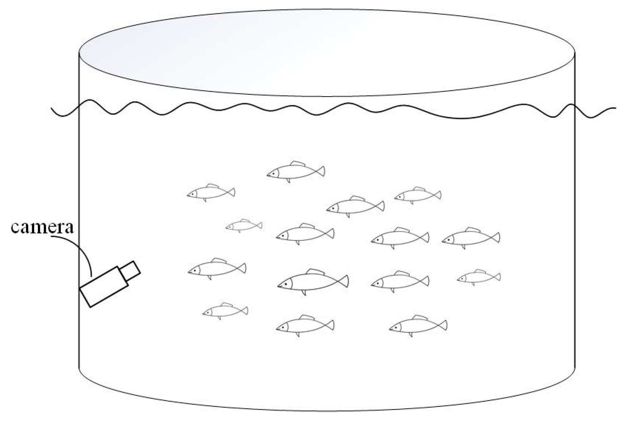
2.1. Experimental Materials
2.2. Dataset
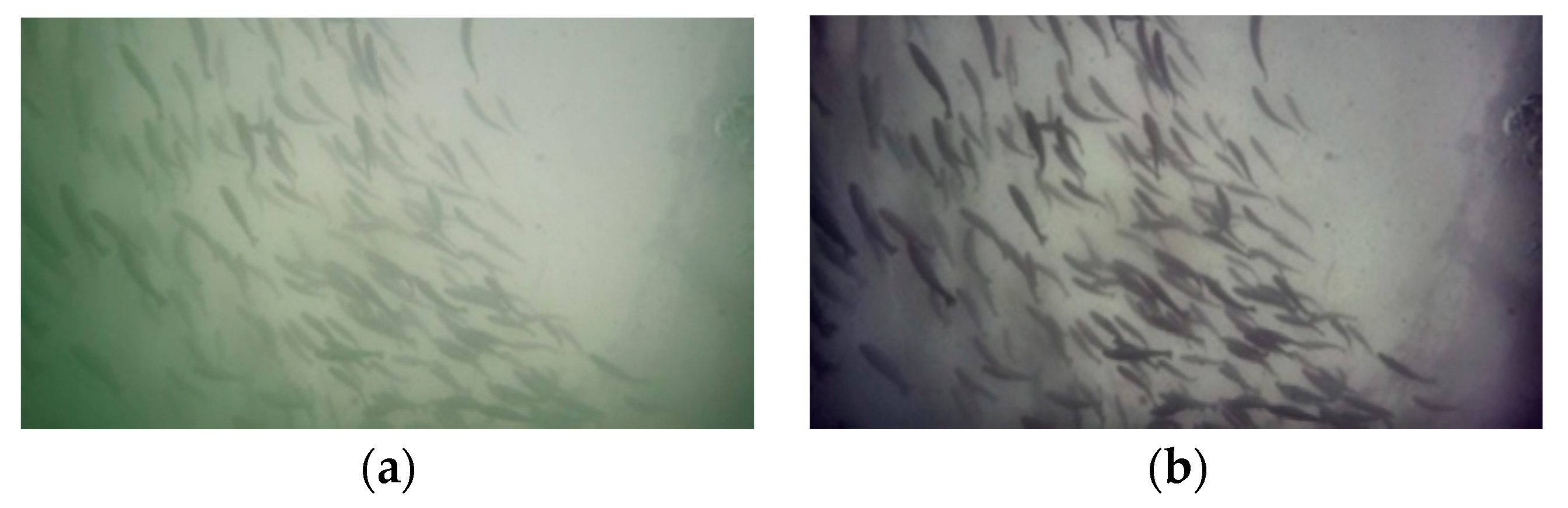
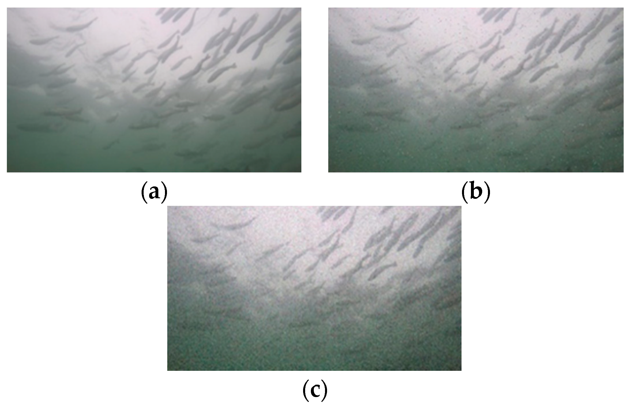
2.2.1. Data Preprocessing and Enhancement
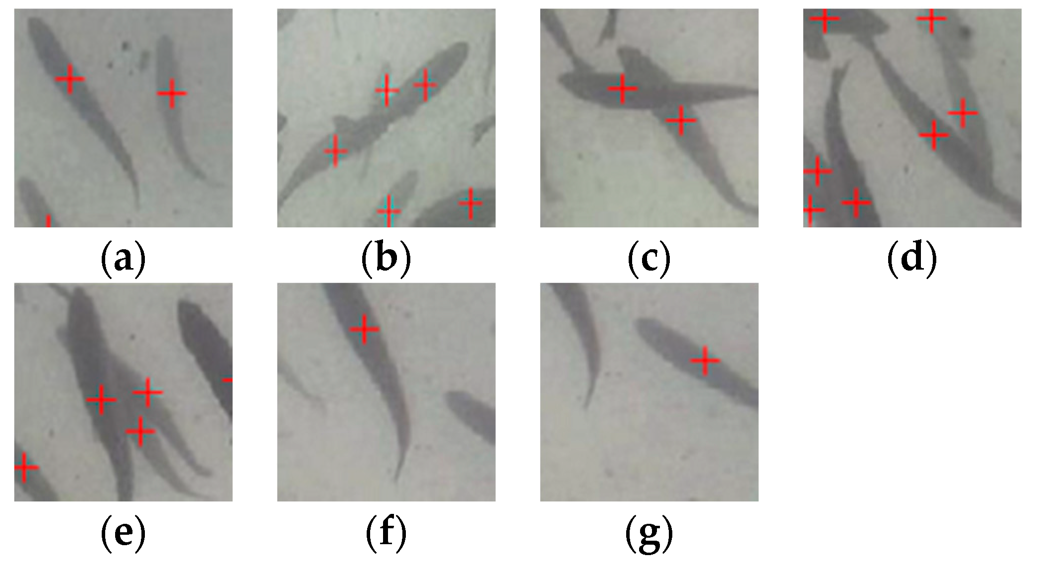
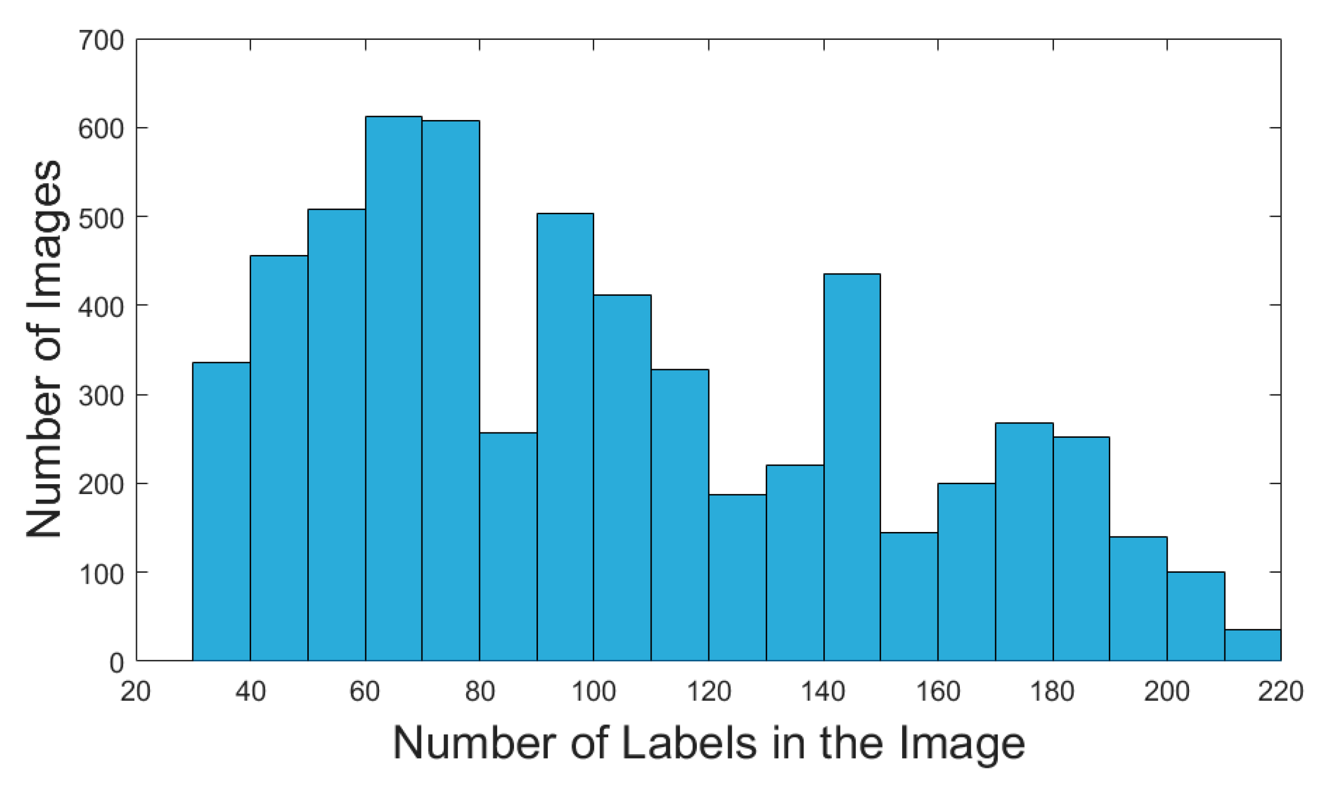
2.2.2. Dataset Production
2.3. Fish Counting based on a Hybrid Neural Network Model
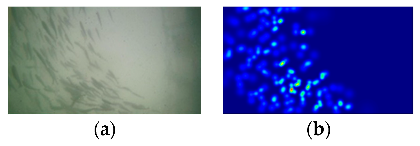
2.3.1. Fish Shoal Density Map
2.3.2. Design of the Hybrid Neural Network
Multi-Column Convolution Neural Network
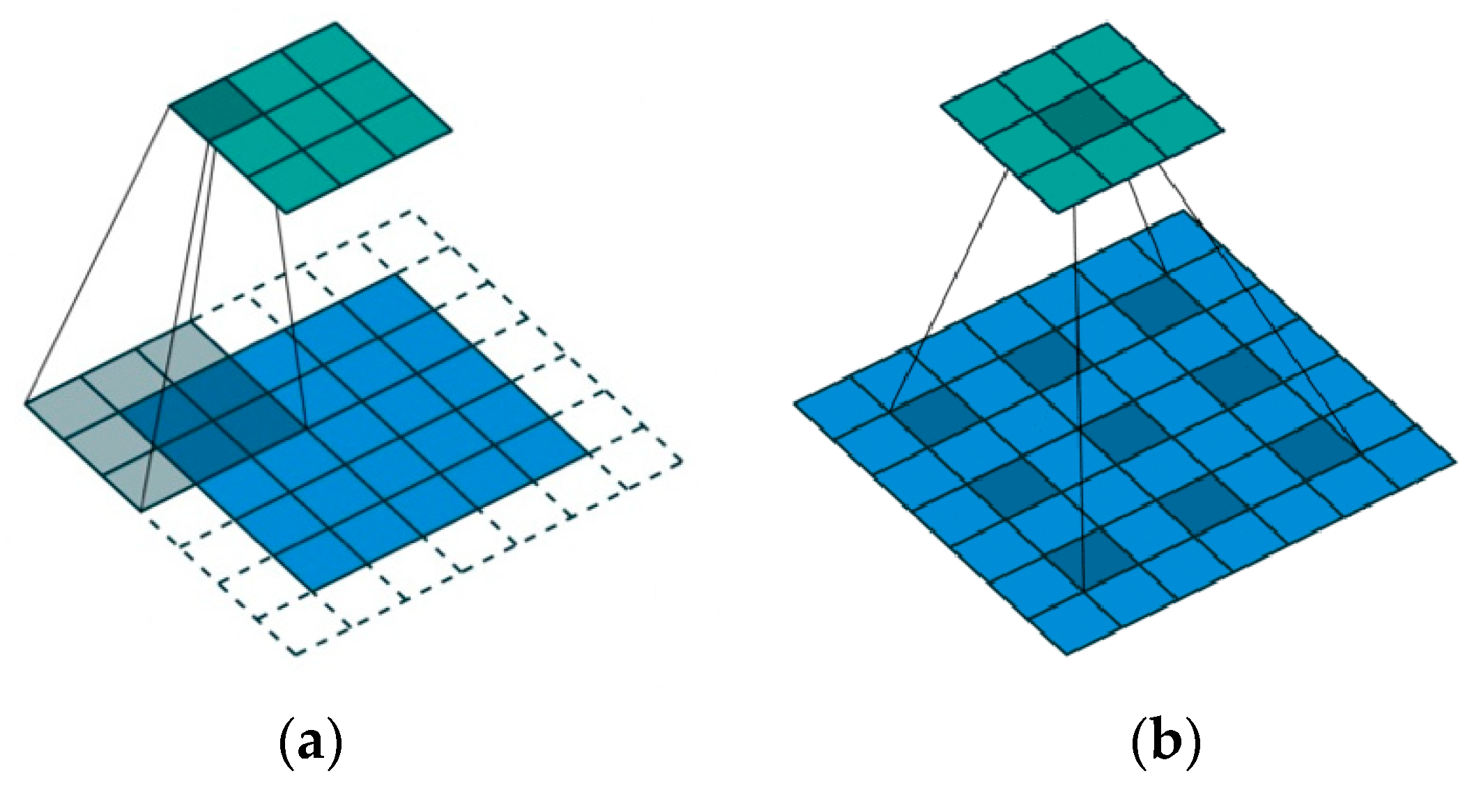
Dilated Convolution Neural Network
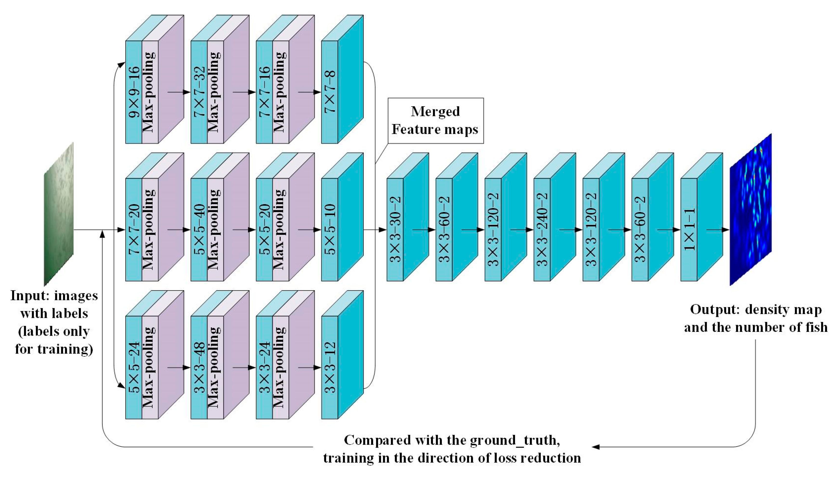
Design of the Hybrid Neural Network
2.4. Model Performance Evaluation Metric
3. Results and Discussions
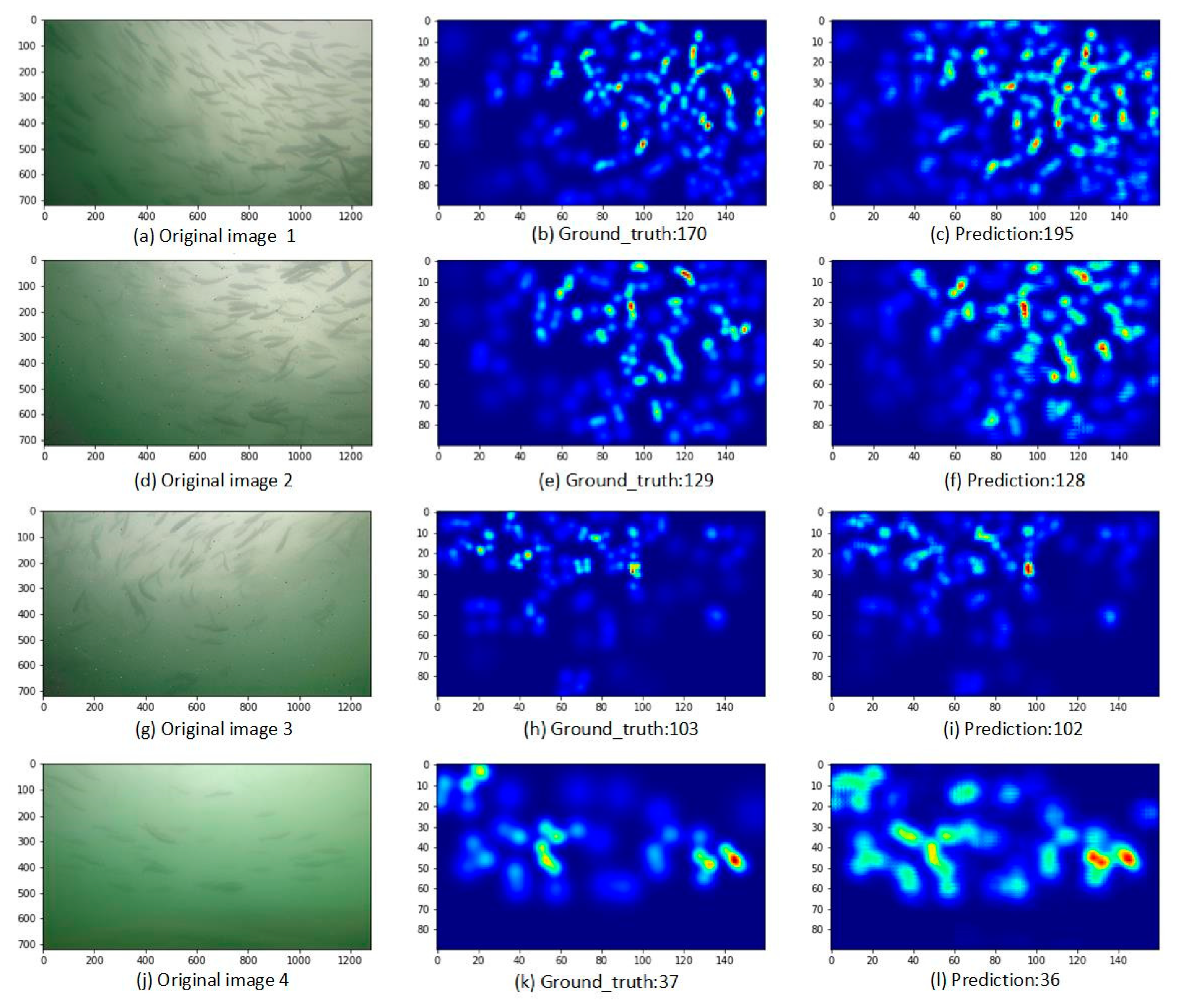
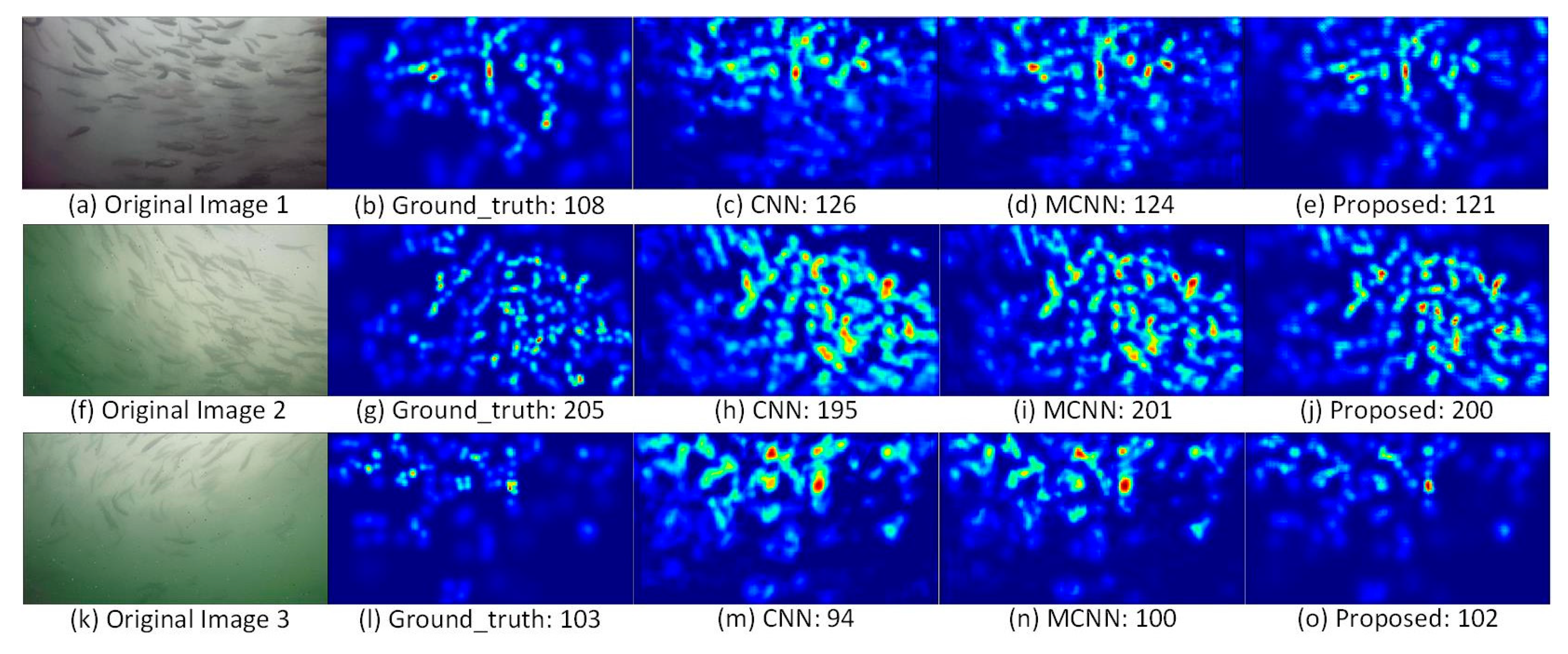
3.1. Results of Fish Counting
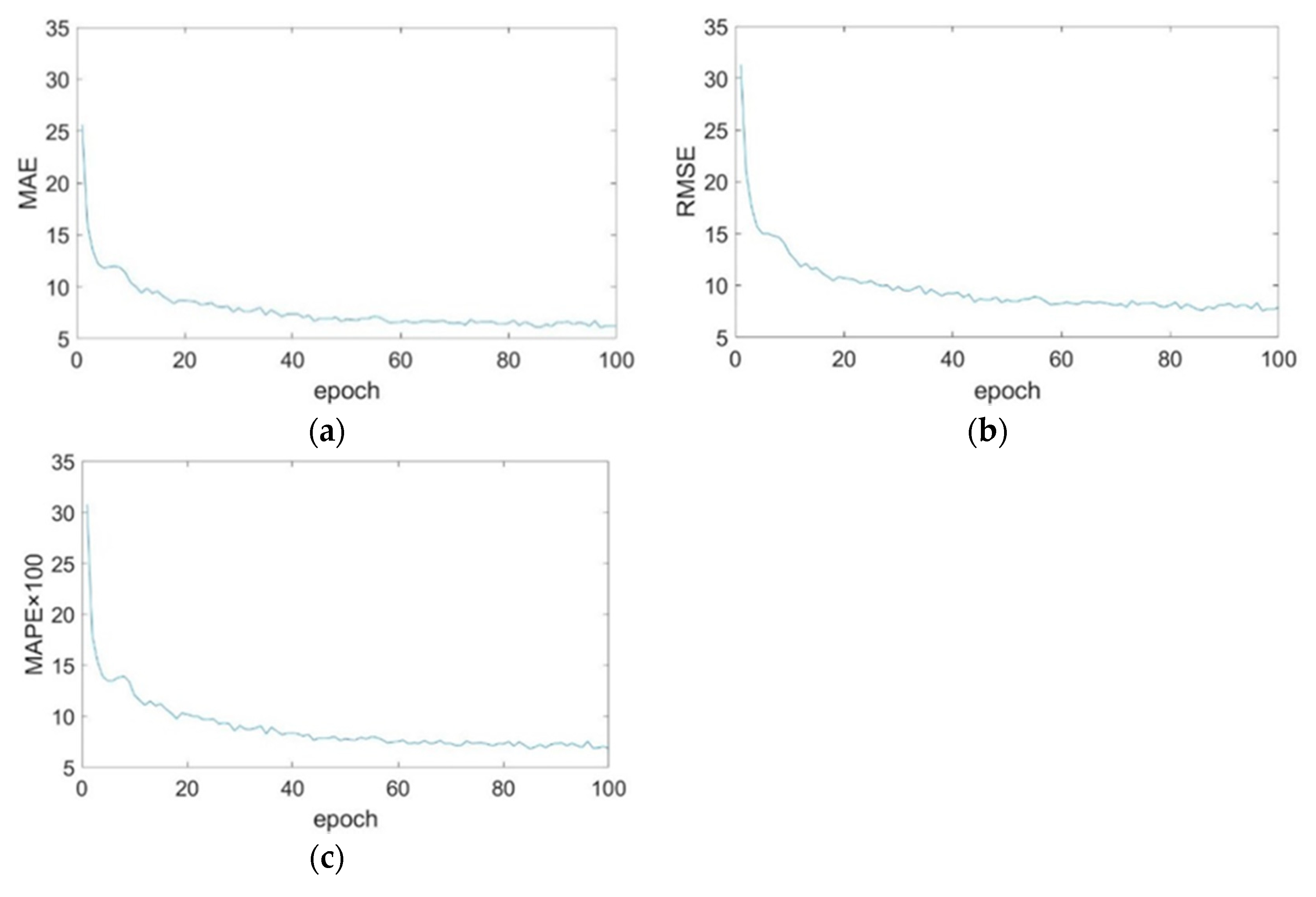
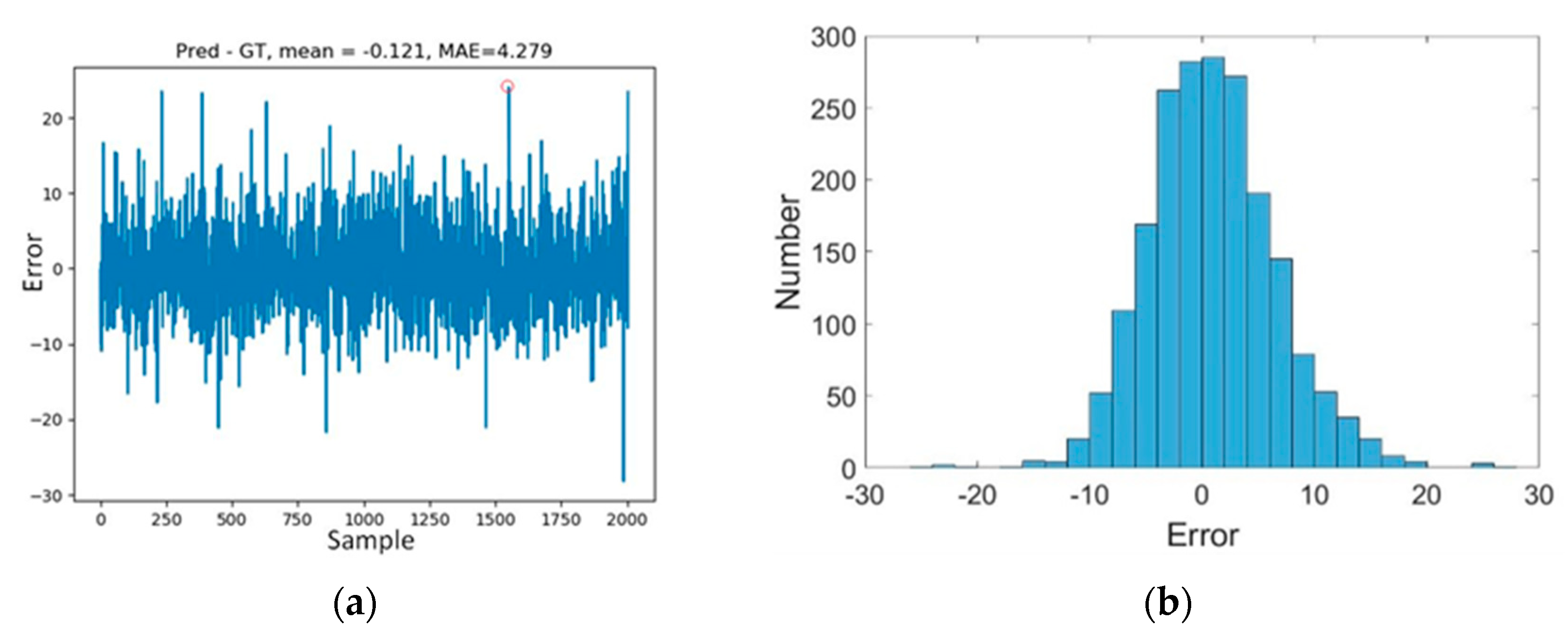
3.2. Discussion on Model Performance
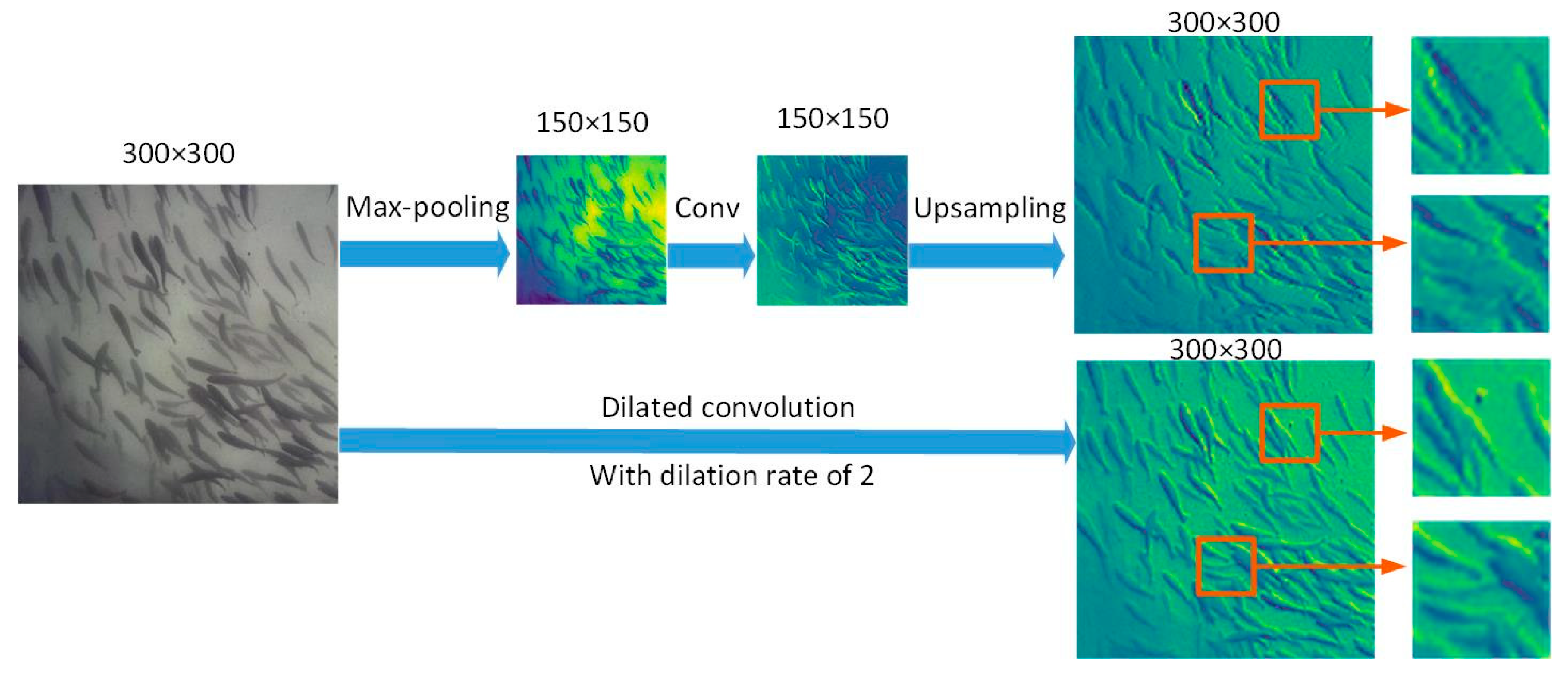
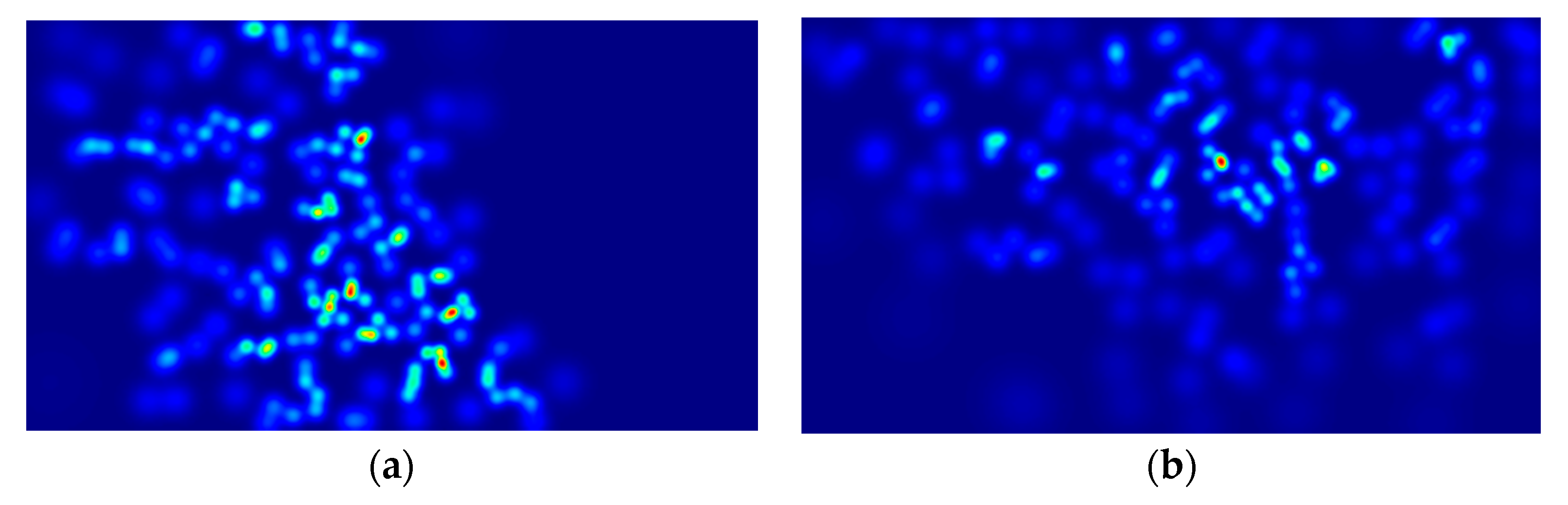
3.2.1. Dilated Convolution Neural Network
3.2.2. Comparison with Other Methods
4. Conclusions
Author Contributions
Funding
Acknowledgments
Conflicts of Interest
References
- Li, D.; Hao, Y.; Duan, Y. Nonintrusive methods for biomass estimation in aquaculture with emphasis on fish: A review. Rev. Aquac. 2019. [Google Scholar] [CrossRef]
- Chang, C.; Fang, W.; Jao, R.-C.; Shyu, C.; Liao, I. Development of an intelligent feeding controller for indoor intensive culturing of eel. Aquacult. Eng. 2005, 32, 343–353. [Google Scholar] [CrossRef]
- Zhou, C.; Lin, K.; Xu, D.; Chen, L.; Guo, Q.; Sun, C.; Yang, X. Near infrared computer vision and neuro-fuzzy model-based feeding decision system for fish in aquaculture. Comput. Electron. Agr. 2018, 146, 114–124. [Google Scholar] [CrossRef]
- Zhou, C.; Zhang, B.; Lin, K.; Xu, D.; Chen, C.; Yang, X.; Sun, C. Near-infrared imaging to quantify the feeding behavior of fish in aquaculture. Comput. Electron. Agr. 2017, 135, 233–241. [Google Scholar] [CrossRef]
- Saberioon, M.; Gholizadeh, A.; Cisar, P.; Pautsina, A.; Urban, J. Application of machine vision systems in aquaculture with emphasis on fish: State-of-the-art and key issues. Rev. Aquac. 2017, 9, 369–387. [Google Scholar] [CrossRef]
- Saberioon, M.; Císař, P.; Labbé, L.; Souček, P.; Pelissier, P.; Kerneis, T. Comparative Performance Analysis of Support Vector Machine, Random Forest, Logistic Regression and k-Nearest Neighbours in Rainbow Trout (Oncorhynchus Mykiss) Classification Using Image-Based Features. Sensors 2018, 18, 1027. [Google Scholar] [CrossRef]
- Toh, Y.; Ng, T.; Liew, B. Automated fish counting using image processing. In Proceedings of the 2009 International Conference on Computational Intelligence and Software Engineering (CiSE2009), IEEE, Wuhan, China, 11–13 December 2009; pp. 1–5. [Google Scholar]
- Labuguen, R.; Volante, E.; Causo, A.; Bayot, R.; Peren, G.; Macaraig, R.; Libatique, N.; Tangonan, G. Automated fish fry counting and schooling behavior analysis using computer vision. In Proceedings of the 2012 IEEE 8th International Colloquium on Signal Processing and its Applications, Malacca, Malaysia, 23–25 March 2012; pp. 255–260. [Google Scholar]
- Fan, L.; Liu, Y. Automate fry counting using computer vision and multi-class least squares support vector machine. Aquaculture 2013, 380, 91–98. [Google Scholar] [CrossRef]
- Canny, J. A computational approach to edge detection. IEEE Trans. Pattern Anal. Mach. Intell. 1986, 679–698. [Google Scholar] [CrossRef]
- Sharma, S.; Shakya, A.; Panday, S.P. Fish Counting from Underwater Video Sequences by Using Color and Texture. Int. J. Sci. Eng. Res. 2016, 7, 1243–1249. [Google Scholar]
- Fabic, J.; Turla, I.; Capacillo, J.; David, L.; Naval, P. Fish population estimation and species classification from underwater video sequences using blob counting and shape analysis. In Proceedings of the 2013 IEEE International Underwater Technology Symposium (UT), Tokyo, Japan, 5–8 March 2013; pp. 1–6. [Google Scholar]
- Le, J.; Xu, L. An automated fish counting algorithm in aquaculture based on image processing. In Proceedings of the 2016 International Forum on Mechanical, Control and Automation (IFMCA 2016), Shenzhen, China, 30–31 December 2017; 113, pp. 358–366. [Google Scholar]
- Albuquerque, P.L.F.; Garcia, V.; Junior, A.d.S.O.; Lewandowski, T.; Detweiler, C.; Gonçalves, A.B.; Costa, C.S.; Naka, M.H.; Pistori, H. Automatic live fingerlings counting using computer vision. Comput. Electron. Agr. 2019, 167, 105015. [Google Scholar] [CrossRef]
- Qiu, J.; Wu, Q.; Ding, G.; Xu, Y.; Feng, S. A survey of machine learning for big data processing. EURASIP J. Adv. Signal Process. 2016, 2016, 67. [Google Scholar] [CrossRef]
- Weiss, K.; Khoshgoftaar, T.M.; Wang, D. A survey of transfer learning. J. Big data 2016, 3, 9. [Google Scholar] [CrossRef]
- Pereira, C.S.; Morais, R.; Reis, M.J. Deep Learning Techniques for Grape Plant Species Identification in Natural Images. Sensors 2019, 19, 4850. [Google Scholar] [CrossRef]
- Zamansky, A.; Sinitca, A.M.; Kaplun, D.I.; Plazner, M.; Schork, I.G.; Young, R.J.; de Azevedo, C.S. Analysis of dogs’ sleep patterns using convolutional neural networks. In Proceedings of the International Conference on Artificial Neural Networks, Munich, Germany, 17–19 September 2019; Springer: Cham, Switzerland, 2019; pp. 472–483. [Google Scholar] [CrossRef]
- Trnovszký, T.; Kamencay, P.; Orješek, R.; Benčo, M.; Sýkora, P. Animal recognition system based on convolutional neural network. Digtal Image Process. Comput. Graph. 2017, 15, 517–525. [Google Scholar] [CrossRef]
- Willi, M.; Pitman, R.T.; Cardoso, A.W.; Locke, C.; Swanson, A.; Boyer, A.; Veldthuis, M.; Fortson, L. Identifying animal species in camera trap images using deep learning and citizen science. Methods Ecol. Evol. 2019, 10, 80–91. [Google Scholar] [CrossRef]
- Måløy, H.; Aamodt, A.; Misimi, E. A spatio-temporal recurrent network for salmon feeding action recognition from underwater videos in aquaculture. Comput. Electron. Agr. 2019, 105087. [Google Scholar] [CrossRef]
- Rauf, H.T.; Lali, M.I.U.; Zahoor, S.; Shah, S.Z.H.; Rehman, A.U.; Bukhari, S.A.C. Visual features based automated identification of fish species using deep convolutional neural networks. Comput. Electron. Agr. 2019, 105075. [Google Scholar] [CrossRef]
- Zhou, C.; Xu, D.; Chen, L.; Zhang, S.; Sun, C.; Yang, X.; Wang, Y. Evaluation of fish feeding intensity in aquaculture using a convolutional neural network and machine vision. Aquaculture 2019, 507, 457–465. [Google Scholar] [CrossRef]
- Salman, A.; Siddiqui, S.A.; Shafait, F.; Mian, A.; Shortis, M.R.; Khurshid, K.; Ulges, A.; Schwanecke, U. Automatic fish detection in underwater videos by a deep neural network-based hybrid motion learning system. ICES J. Mar. Sci. 2019. [Google Scholar] [CrossRef]
- Shelhamer, E.; Long, J.; Darrell, T. Fully Convolutional Networks for Semantic Segmentation. IEEE Trans. Pattern Anal. Mach. Intell. 2017, 4, 640–651. [Google Scholar] [CrossRef]
- Qin, Y.; Wu, Y.; Li, B.; Gao, S.; Liu, M.; Zhan, Y. Semantic Segmentation of Building Roof in Dense Urban Environment with Deep Convolutional Neural Network: A Case Study Using GF2 VHR Imagery in China. Sensors 2019, 19, 1164. [Google Scholar] [CrossRef] [PubMed]
- Zhang, Y.; Zhou, D.; Chen, S.; Gao, S.; Ma, Y. Single-image crowd counting via multi-column convolutional neural network. In Proceedings of the IEEE conference on computer vision and pattern recognition, Las Vegas, NV, USA, 26 June–1 July 2016; pp. 589–597. [Google Scholar]
- Perone, C.S.; Calabrese, E.; Cohen-Adad, J. Spinal cord gray matter segmentation using deep dilated convolutions. Sci. Rep. 2018, 8, 5966. [Google Scholar] [CrossRef] [PubMed]
- Fu, X.; Fan, Z.; Ling, M.; Huang, Y.; Ding, X. Two-step approach for single underwater image enhancement. In Proceedings of the 2017 International Symposium on Intelligent Signal Processing and Communication Systems (ISPACS), Xiamen, China, 6–9 November 2017; pp. 789–794. [Google Scholar]
- Buchsbaum, G. A spatial processor model for object colour perception. J. Franklin Inst. 1980, 310, 1–26. [Google Scholar] [CrossRef]
- Jiang, B.; Wu, Q.; Yin, X.; Wu, D.; Song, H.; He, D. FLYOLOv3 deep learning for key parts of dairy cow body detection. Comput. Electron. Agr. 2019, 166, 104982. [Google Scholar] [CrossRef]
- Dollar, P.; Wojek, C.; Schiele, B.; Perona, P. Pedestrian detection: An evaluation of the state of the art. IEEE Trans. Pattern Anal. Mach. Intell. 2011, 34, 743–761. [Google Scholar] [CrossRef]
- Chan, A.B.; Vasconcelos, N. Bayesian poisson regression for crowd counting. In Proceedings of the 2009 IEEE 12th international conference on computer vision, CenterKyoto, Japan, 29 September–2 October 2009; pp. 545–551. [Google Scholar]
- Lempitsky, V.; Zisserman, A. Learning to count objects in images. In Proceedings of the 23rd International Conference on Neural Information Processing Systems, Vancouver, BC, Canada, 6–9 December 2010; pp. 1324–1332. [Google Scholar]
- Yang, X.; Sun, H.; Fu, K.; Yang, J.; Sun, X.; Yan, M.; Guo, Z. Automatic ship detection in remote sensing images from google earth of complex scenes based on multiscale rotation dense feature pyramid networks. Remote Sens. 2018, 10, 132. [Google Scholar] [CrossRef]
- Chen, L.-C.; Papandreou, G.; Kokkinos, I.; Murphy, K.; Yuille, A.L. Deeplab: Semantic image segmentation with deep convolutional nets, atrous convolution, and fully connected crfs. IEEE Trans. Pattern Anal. Mach. Intell. 2017, 40, 834–848. [Google Scholar] [CrossRef]
- Lin, G.; Wu, Q.; Qiu, L.; Huang, X. Image super-resolution using a dilated convolutional neural network. Neurocomputing 2018, 275, 1219–1230. [Google Scholar] [CrossRef]
- Aghdam, H.H.; Heravi, E.J.; Puig, D. A practical approach for detection and classification of traffic signs using convolutional neural networks. Rob. Auton. Syst. 2016, 84, 97–112. [Google Scholar] [CrossRef]
- Dumoulin, V.; Visin, F. A guide to convolution arithmetic for deep learning. Statistical 2018, 1050, 11. [Google Scholar]
- Simonyan, K.; Zisserman, A. Very Deep Convolutional Networks for Large-Scale Image Recognition. Comput. Sci. 2014, 1409, 1556. [Google Scholar]
- Zhang, S.; Zhang, S.; Zhang, C.; Wang, X.; Shi, Y. Cucumber leaf disease identification with global pooling dilated convolutional neural network. Comput. Electron. Agr. 2019, 162, 422–430. [Google Scholar] [CrossRef]
- Oppedal, F.; Dempster, T.; Stien, L.H. Environmental drivers of Atlantic salmon behaviour in sea-cages: A review. Aquaculture 2011, 311, 1–18. [Google Scholar] [CrossRef]


| Parameter Name | Set Up | Parameter Name | Set Up |
|---|---|---|---|
| optimization algorithm | Adam | learning rate | 1e-5 |
| Gauss initialization | 0.01 standard deviation | loss function | MSE in Keras |
| epoch | 100 | batch size | 1 (online learning) |
| activation function | ReLU | padding | same |
| Range Name | Range | Number | Accuracy |
|---|---|---|---|
| Fewer | <60 | 468 | 93.43% |
| Few | [60, 100) | 656 | 94.21% |
| Medium | [100, 140) | 376 | 95.77% |
| Many | [140, 180) | 360 | 97.02% |
| Large | ≥180 | 144 | 97.55% |
| Method | Metrics | |||
|---|---|---|---|---|
| MAE | RMSE | MAPE | Accuracy | |
| CNN | 8.85 | 11.37 | 10.39 | 89.61% |
| MCNN | 7.85 | 10.10 | 8.82 | 91.18% |
| Proposed | 4.29 | 5.57 | 4.94 | 95.06% |
© 2020 by the authors. Licensee MDPI, Basel, Switzerland. This article is an open access article distributed under the terms and conditions of the Creative Commons Attribution (CC BY) license (http://creativecommons.org/licenses/by/4.0/).
Share and Cite
Zhang, S.; Yang, X.; Wang, Y.; Zhao, Z.; Liu, J.; Liu, Y.; Sun, C.; Zhou, C. Automatic Fish Population Counting by Machine Vision and a Hybrid Deep Neural Network Model. Animals 2020, 10, 364. https://doi.org/10.3390/ani10020364
Zhang S, Yang X, Wang Y, Zhao Z, Liu J, Liu Y, Sun C, Zhou C. Automatic Fish Population Counting by Machine Vision and a Hybrid Deep Neural Network Model. Animals. 2020; 10(2):364. https://doi.org/10.3390/ani10020364
Chicago/Turabian StyleZhang, Song, Xinting Yang, Yizhong Wang, Zhenxi Zhao, Jintao Liu, Yang Liu, Chuanheng Sun, and Chao Zhou. 2020. "Automatic Fish Population Counting by Machine Vision and a Hybrid Deep Neural Network Model" Animals 10, no. 2: 364. https://doi.org/10.3390/ani10020364
APA StyleZhang, S., Yang, X., Wang, Y., Zhao, Z., Liu, J., Liu, Y., Sun, C., & Zhou, C. (2020). Automatic Fish Population Counting by Machine Vision and a Hybrid Deep Neural Network Model. Animals, 10(2), 364. https://doi.org/10.3390/ani10020364