Investigating the Ability of Growth Models to Predict In Situ Vibrio spp. Abundances

Abstract

Vibrio spp. have an important role in biogeochemical cycles; some species are disease agents for aquatic animals and/or humans. Predicting population dynamics of Vibrio spp. in natural environments is crucial to predicting how the future conditions will affect the dynamics of these bacteria. The majority of existing Vibrio spp. population growth models were developed in controlled environments, and their applicability to natural environments is unknown. We collected all available functional models from the literature, and distilled them into 28 variants using unified nomenclature. Next, we assessed their ability to predict Vibrio spp. abundance using two new and five already published longitudinal datasets on Vibrio abundance in four different habitat types. Results demonstrate that, while the models were able to predict Vibrio spp. abundance to an extent, the predictions were not reliable. Models often underperformed, especially in environments under significant anthropogenic influence such as aquaculture and urban coastal habitats. We discuss implications and limitations of our analysis, and suggest research priorities; in particular, we advocate for measuring and modeling organic matter.

1. Introduction

Vibrio spp. are naturally occurring aquatic bacteria, highly adaptive and freely associated with a variety of biotic and abiotic surfaces including water, sediment, fish, shellfish, algae, and zooplankton. Vibrio spp. comprise a minor portion of the total microbial population, and around 1 percent of the total bacterioplankton in coastal waters [1]. Despite their relatively low abundance, Vibrio species are one of key constituents of aquatic heterotrophic bacterial groups [2].

Aquatic heterotrophic microorganisms have an important role in the mineralization of organic matter, and the variations in abundance, community structure, and activities of heterotrophic microbial communities affect both the biotic and the abiotic components of aquatic environments. Vibrio spp. participate in biogeochemical processes by utilizing a variety of substrates and mineralization of organic matter, thus directly contributing to the recycling of carbon, nitrogen, and organic matter in the aquatic environment [1,3,4]. Alongside their role in the abiotic cycles, some >140 described species from the genus Vibrio can have a strong biotic impact, and consequently pose severe health risks and economic losses. A well-known example is Vibrio cholerae, which causes cholera—a global threat to public health with about four million cases of infection every year, leading to over 100,000 deaths [5]. The rise of noncholera Vibrio species (V. parahaemolyticus, V. alginolyticus, and V. vulnificus) can cause other potentially lethal infections (vibriosis) in humans [2], and some of the well-known Vibrio pathogens (e.g., V. anguillarum, V. harveyi, V. vulnificus, V. salmonicida) are harmful to aquatic (marine) organisms; these species induce vibriosis in fish and other marine species, which results in massive economic losses for the aquaculture industry worldwide.

Outbreaks of vibriosis naturally arise mainly with fluctuations in the physicochemical properties of water such as temperature, salinity, dissolved oxygen, and nutrient pulses (e.g., phytoplankton blooms and dust storms). Fluctuations are supported by the fast response of Vibrio spp. to favorable environmental conditions [6,7]. The ongoing climate change adds complexity to the environmental patterns, as it induces shifts in the marine environments by increasing temperature, altering nutrient loads, shifting precipitation patterns, and acidifying the ocean [8,9,10]. This, in turn, affects the Vibrio spp. abundance and alters the distribution of infectious diseases such as vibriosis [11]. Climate change can also initiate the lengthening of the seasonal period of maximal Vibrio concentrations and broaden the areas permitting the survival of these pathogens [12]. Therefore, in order to develop informed strategies to minimize vibriosis outbreaks and prevent potential health risks and aquaculture economic losses, it is crucial to take both Vibrio spp. dynamics and the environment into account.

Mathematical modeling, analysis, and simulations provide useful insights into Vibrio spp. abundance in various natural or anthropogenic systems. They help in developing management strategies, and advance the knowledge of changes in the microbial communities in aquatic environments. Accurate predictions can also advance the decision-making processes of aquaculture and estimation of costs, as well as the enactment of legislation in food safety and water research, which are two major areas in applied microbiology [13,14]. The main approach to modeling the Vibrio spp. is based on empirical techniques, where models are analyzed from statistical, numerical, and computational points of view, such as goodness of fit or standard errors of the estimated parameters. Mathematical models in food safety research (e.g., [15,16,17,18]) are generally categorized into primary, secondary, and tertiary models [19].

Microbial growth curves show the number of living cells as a function of time [17]. Primary models typically describe isothermal growth, i.e., growth as a function of time at a constant temperature. Under constant (laboratory) conditions, bacterial growth is characterized by a sigmoid curve where the dependent variable is the logarithm of the viable cell concentration [20]. The slope of a sigmoid curve at a given time provides the instantaneous specific growth rate, which can be considered as the “cells’ per capita rate of division” [21]. The other two essential parameters of primary models are the maximum specific growth rate at the inflexion point of the sigmoid curve, and the length of the lag phase.

Secondary mathematical models describe the functional dependence of microbial growth on external factors such as temperature or pH [17]. Commonly used secondary models are the square-root model (Ratkowsky model [22]) and the Arrhenius-based model [23], which provide satisfactory descriptions of the dependence of growth on temperature, pH, or other factors [24]. Finally, tertiary mathematical models are software packages that combine primary and/or secondary models and often add a user interface [24].

Generally, all described models are useful, but they are not always applicable. The described mathematical models can be used for description and prediction of Vibrio spp. abundance only under certain (known and tested) conditions. The limitations stem from model formulation: while the equations provide satisfactory descriptions of Vibrio growth and its dependence on, e.g., temperature or pH, they usually are not subject to mechanistic interpretation [24], and therefore should not be used for explanatory purposes or predictions under untested conditions. The issue of the applicability and usability of a model becomes important when we wish to apply a model to understand or predict Vibrio spp. dynamics in situ. For data collected in situ, exact conditions of data collection are unknown, intervals between data collection are long and/or irregular, and environmental conditions are rarely constant.

We aimed to (i) identify and systematize primary and secondary Vibrio spp. growth models, and (ii) to analyze and validate the models by applying them to different sets of available data. We reviewed growth models of Vibrio spp. using examples from research in food safety and water research, and validated them on several sets of field data. Then, we analyzed whether the model(s) can be used to capture in situ Vibrio spp. abundances, with  an emphasis on differences between the marine habitat types.

2. Materials and Methods

Our methodological approach can be divided into four main steps: (1) a literature search, (2) data preparation, (3) model simulations, and (4) performance analysis. The methodology overview is graphically presented in Figure 1.

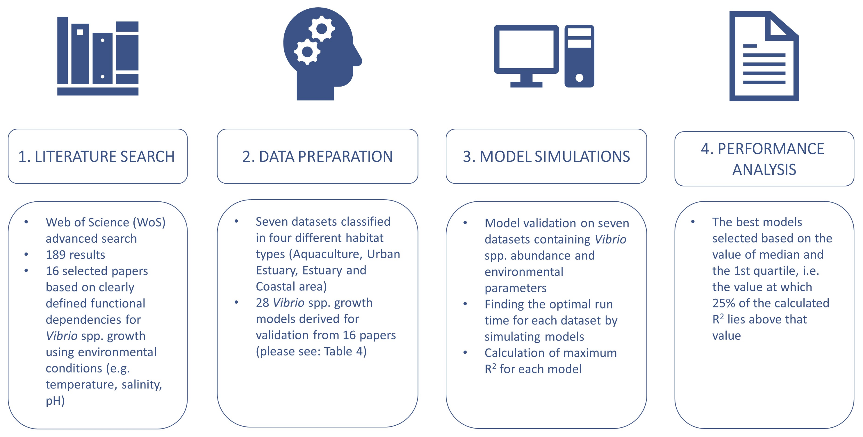
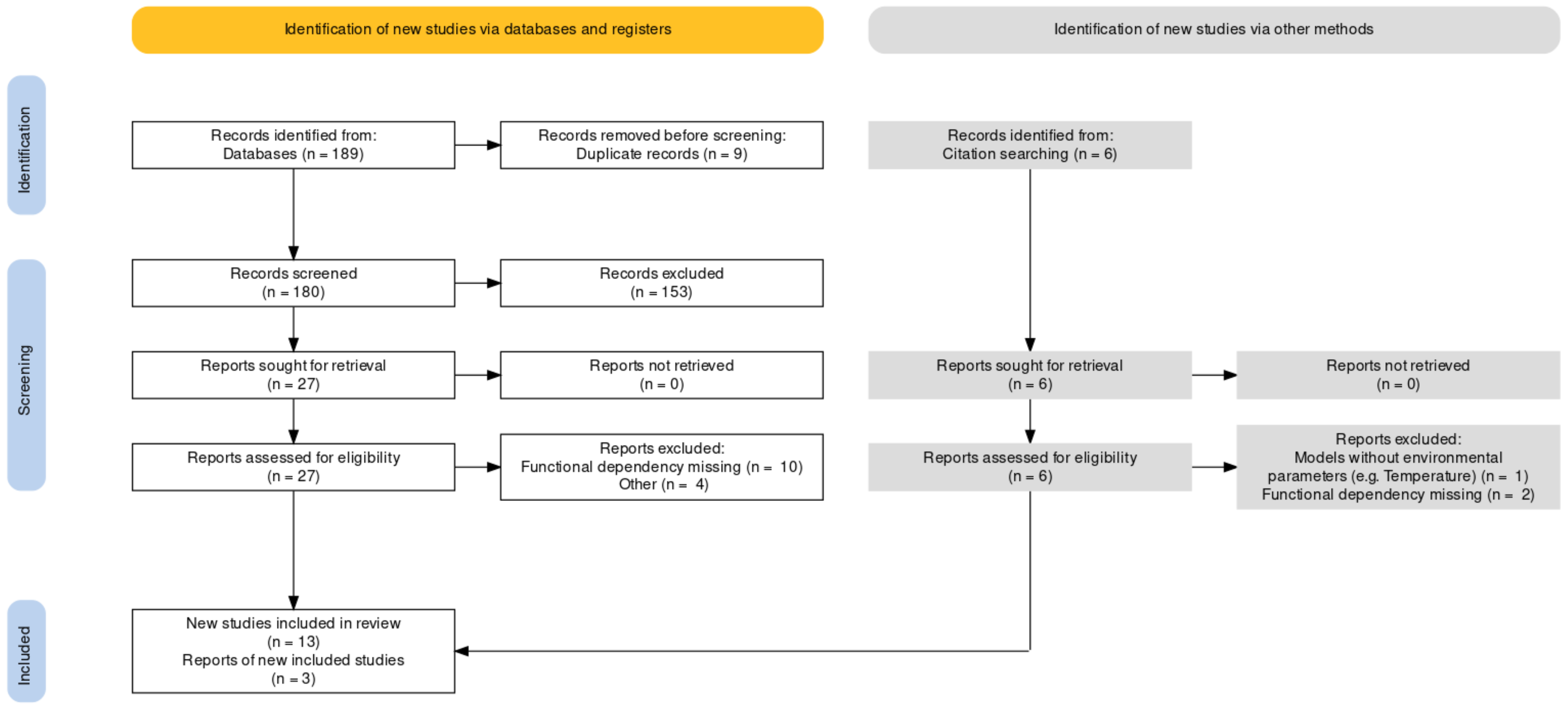
2.1. Literature Search and Model Synthesis

The literature search was conducted using the Web of Science (WoS) advanced search in April 2022. The search string was defined based on keywords and Boolean and adjacency operators, and was searched for in Abstracts (Field Tag “AB”). The search string was as follows: AB = (((vibrio*) AND (growth OR abundance) AND (temperature OR salinity OR “pH” OR “COD” OR “organic matter” OR nutrient*) AND (model*))). We obtained 189 results based on our search, which was restricted to the English language. For  a detailed description of our literature review, please see Appendix A. We selected 16 papers with Vibrio spp. growth models based on clearly defined functional dependencies for using environmental conditions (e.g., temperature, salinity, pH). We did not include models derived purely by regression or similar statistical means because those are not modular, and cannot be differentiated into primary and secondary. From the 16 papers containing growth models, we extracted, systematized, and classified explicit formulations for primary (

Table 1. Systematized equations for Vibrio spp. primary growth models. Of the 12 models listed in this table, one (new logistic model) did not have parameters listed, so only the remaining 11 were used in further analysis. The reference in the column “Model” is the original paper containing the equation. The column “Article” lists all published articles that used the given primary models.

Model	Equation	Article
Modified logistic [25]	$$Y\left(t\right)=\frac{A}{\left\{1+\exp \left[\frac{4·{\mu }_{\max }}{A}\left(\lambda -t\right)+2\right]\right\}}$$ (1)	[26,27,28,29]
Baranyi [30]	$$\left\{\begin{array}{c}Y\left(t\right)=Y_0+{\mu }_{max}\mathrm{A}\left(\mathrm{t}\right)-ln[1+\frac{exp\left({\mu }_{max}\mathrm{A}\left(t\right)\right)-1}{exp(Y_{max}-Y_0)}]\\ \mathrm{A}\left(\mathrm{t}\right)=t+\frac{1}{{\mu }_{max}}ln\left[exp\left(-{\mu }_{max}t\right)+exp\left(-{\mu }_{max}\lambda \right)-exp\left(-{\mu }_{max}t-{\mu }_{max}\lambda \right)\right]\end{array}\right.$$ (2)	[26,28,29,31,32,33,34,35,36,37]
Gompertz [25]	$$Y\left(t\right)=Y_0+A\left(e^{\left(-e^{-B\left(t-D\right)}\right)}\right)$$ (3)	[37,38,39]
Modified Gompertz [25]	$$Y\left(t\right)=Y_0+Aexp\left\{-exp\left[\frac{{\mu }_{max}·e}{A}\left(\lambda -t\right)+1\right]\right\}$$ (4)	[28,29,31,40,41,42]
Weibull [43]	$$Y\left(t\right)=Y_0-{\left(\frac{t}{\delta }\right)}^p$$ (5)	[28,41]
Three-phase linear [44]	$$\left\{\begin{array}{c}Y\left(t\right)=Y_0,t\le \lambda \\ Y\left(t\right)=Y_0+{\mu }_{max}\left(t-\lambda \right),\lambda <t<t_s\\ Y\left(t\right)=Y_{max},t\ge t_s\end{array}\right.$$ (6)	[29,45]
Huang [46]	$$\left\{\begin{array}{c}Y\left(t\right)=Y_0+Y_{max}-ln\left\{exp\left(Y_0\right)+\left[exp\left(Y_{max}\right)-exp\left(Y_0\right)\right]exp\left(-{\mu }_{max}\mathrm{B}\left(\mathrm{t}\right)\right)\right\}\\ \mathrm{B}\left(\mathrm{t}\right)=t+\frac{1}{4}ln\frac{1+exp\left[-4\left(t-\lambda \right)\right]}{1-exp\left(4\lambda \right)}\end{array}\right.$$ (7)	[29,47]
No-lag phase [48]	$$Y\left(t\right)=Y_0+Y_{max}-ln\left\{exp\left(Y_0\right)+\left[exp\left(Y_{max}\right)-exp\left(Y_0\right)\right]exp\left(-{\mu }_{max}t\right)\right\}$$ (8)	[47]
Net exponential	$$Y\left(t\right)=Y_0·e^{\mu t}$$ (9)	[49]
Modified Richards [25]	$$Y\left(t\right)=A{\left\{1+\nu ·exp\left(1+\nu \right)·exp\left[\frac{{\mu }_{max}}{A}\left(1+\nu \right)\left(1+\frac{1}{\nu }\right)·\left(\lambda -t\right)\right]\right\}}^{\left(-\frac{1}{\nu }\right)}$$ (10)	[29]
Modified Schnute [25]	$$Y\left(t\right)=\left({\mu }_{max}\frac{\left(1-b\right)}{a}\right){\left[\frac{1-b·exp\left(a·\lambda +1-b-at\right)}{1-b}\right]}^{\frac{1}{b}}$$ (11)	[29]
New logistic [50]	$$\frac{\mathrm{d}Y}{\mathrm{d}t}={\mu }_{max}Y\left\{1-{\left(\frac{Y}{Y_{max}}\right)}^m\right\}\left\{1-{\left(\frac{Y_{min}}{Y}\right)}^n\right\}$$ (12)	[51]

) and secondary growth models (

Table 2. Systematized equations for Vibrio spp. secondary growth models. These models modify specific growth rate and lag time in primary models to capture effects of environmental conditions such as temperature, salinity, and pH.

Model	Equation	Article
Square root [52]	$${\mu }_{max}={\left[a\left(T-T_{min}\right)\right]}^2$$ (13)	[26,33,35,40,41,45]
Polynomial model	$$\lambda or{\mu }_{max}=a+a_{1}T+a_2{T}^2+\dots +a_n{T}^n$$ (14)	[32,34,36,51]
Response surface [37]	$$\begin{array}{c}{\mu }_{max}or1/\lambda =exp(C_0+C_1·T+C_2·a_w\\ +C_3·T·a_w+C_4·T^2+C_5·a_w^2)\end{array}$$ (15)	[37]
Arrhenius-based [23]	$${\mu }_{max}=\exp \left(C_0+\frac{C_1}{T}+\frac{C_2}{T^2}+C_3{a}_w+C_4{a}_w^2\right)$$ (16)	[31,37,40,42]
Modified Ratkovsky [22]	$${\mu }_{max}=b{\left(T-T_{min}\right)}^2\left\{1-exp\left[c\left(T-T_{max}\right)\right]\right\}$$ (17)	[31]
Suboptimal Huang square root [53]	$${\mu }_{max}={\left[a{\left(T-T_{min}\right)}^{0.75}\right]}^2$$ (18)	[47]
Four-parameter square root and water activity [38]	$$\begin{array}{c}{\mu }_{max}={\left(b\left(T-T_{min}\right)\left\{1-exp\left[c\left(T-T_{max}\right)\right]\right\}\right)}^2\\ ·\left(a_w-a_{wmin}\right)\left\{1-exp\left[d\left(a_w-a_{wmax}\right)\right]\right\}\end{array}$$ (19)	[38]
Net Vibrio growth rate [49]	$$\begin{array}{c}{\mu }_{\nu }=[{\mu }_{max}\ast \mathrm{fn}(S,S_{\mathrm{opt}},S_{\mathrm{width}})-k_d]\ast {\theta }^{T-20},\mathrm{with}\hfill \\ \mathrm{fn}(S,S_{\mathrm{opt}},S_{\mathrm{width}})=\frac{-{\left(S-S_{\mathrm{opt}}\right)}^2}{e^2{\left(S_{\mathrm{width}}\right)}^2},\mathrm{if}\hfill \\ S<S_{\mathrm{opt}}-0.5·S_{\mathrm{width}},\mathrm{or}\hfill \\ S>S_{\mathrm{opt}}-0.5·S_{\mathrm{width}}\hfill \end{array}$$ (20)	[49]

), using parameters listed in (

Table 3. Parameters used in Vibrio spp. primary and secondary models. Last column lists models using the particular parameter.

Parameter	Description	Used in Model
$Y\left(t\right)$ $Y_0$ $Y_{max}$	Logarithm of real-time initial and maximum bacterial counts	All primary models
${\mu }_{max}$	Maximum specific growth rate	All primary models except Weibull and New logistic All secondary models except Net Vibrio growth rate
${\mu }_{\nu }$	Net Vibrio growth rate	Net Vibrio growth rate
$\lambda$	Lag time	All primary models except Gompertz, Weibull and New logistic
t	Time	All models
$t_s$	Time to reach stationary growth phase	Three-phase linear
A	Maximum increase in microbial cell density	Modified logistic Gompertz Modified Gompertz Modified Richards Modified Schnute
B, D	Maximum relative growth rate and time at which the absolute growth rate is maximum	Gompertz
$\nu$	Shape parameter	Modified Richards
a, b, c, m, n	Fitted coefficients	Modified Schnute and New logistic model
$C_0,C_1,C_2$ $C_3,C_4,C_5$	Fitted coefficients	Response surface and Arrhenius-based
T, $T_{min}$, $T_{max}$	Temperature, minimum and maximum temperature required for growth of the organism	All secondary models
$\delta$, p	Coefficients in the Weibull model	Weibull
$a_w,a_{wmin},a_{wmax}$	Optimal, the minimum, and maximum water activity	Four-parameter
$S,S_{\mathrm{opt}},S_{\mathrm{width}}$	Salinity, optimal salinity value, and salinity range for optimal growth	Net Vibrio growth rate

) and thus arriving at 28 unique Vibrio spp. growth models for further analysis (

Table 4. List of models used in the analysis. For each model, Vibrio spp. is specified along with the environment where the growth of the organism was observed. The primary model defines growth function and the secondary model describes functional dependencies accounting for environmental conditions (temperature, salinity, and pH). “Temp” stands for temperature, “Sal” for salinity represented in models as the concentration of NaCl (% NaCl), and “Sal (w.a.)” stands for water activity calculated from salinity. In simulations, salinity from datasets was converted to water activity when needed.

Derived Model	Vibrio spp.	Environment	Environmental Conditions	Primary Model	Secondary Model
Model 1 [26]	V. cholerae	Sea water	Temp	Modified logistic	Square root
Model 2 [26]	V. cholerae	Sea water	Temp	Baranyi	Square root
Model 3 [32]	V. parahaemolyticus	Soy sauce	Temp	Baranyi	Polynomial
Model 4 [33]	V. parahaemolyticus	C. gigas	Temp	Baranyi	Square root
Model 5 [35]	V. parahaemolyticus	C. virginica	Temp	Baranyi	Square root
Model 6 [36]	V. cocktail 1	Table Olives	pH and Sal	Baranyi	Polinomial
Model 7 [34]	V. cholerae and V. vulnificus	O. minor	Temp	Baranyi	Polinomial
Model 8 [37]	V. harveyi	TSYEB 2	Temp and Sal (w.a.)	Baranyi	Response surface
Model 9 [37]	V. harveyi	TSYEB 2	Temp and Sal (w.a.)	Baranyi	Arrhenius-based
Model 10 [31]	V. parahaemolyticus	L. vannamei	Temp	Baranyi	Modified Ratkowsky
Model 11 [37]	V. harveyi	TSYEB 2	Temp and Sal (w.a.)	Gompertz	Response surface
Model 12 [37]	V. harveyi	TSYEB 2	Temp and Sal (w.a.)	Gompertz	Arrhenius-based
Model 13 [38]	V. parahaemolyticus	Model broth system	Temp and Sal (w.a.)	Gompertz	The four-parameter square root
Model 14 [31]	V. parahaemolyticus	L. vannamei	Temp	Modified Gompertz	Modified Ratkowsky
Model 15 [40]	V. parahaemolyticus	Broth	Temp	Modified Gompertz	Square root Arrhenius-based
Model 16 [40]	V. vulnificus	Broth	Temp	Modified Gompertz	Square root Arrhenius-based
Model 17 [40]	V. parahaemolyticus	Flounder sashimi	Temp	Modified Gompertz	Square root Arrhenius-based
Model 18 [40]	V. parahaemolyticus	Salmon sashimi	Temp	Modified Gompertz	Square root Arrhenius-based
Model 19 [40]	V. vulnificus	Oyster meat	Temp	Modified Gompertz	Square root Arrhenius-based
Model 20 [42]	V. parahaemolyticus3	C. gigas broth	Temp	Modified Gompertz	Square root Arrhenius-based
Model 21 [42]	V. parahaemolyticus4	C. gigas broth	Temp	Modified Gompertz	Square root Arrhenius-based
Model 22 [42]	V. parahaemolyticus3	C. gigas Oyster slurry	Temp	Modified Gompertz	Square root Arrhenius-based
Model 23 [42]	V. parahaemolyticus4	C. gigas Oyster slurry	Temp	Modified Gompertz	Square root Arrhenius-based
Model 24 [41]	V. parahaemolyticus	Oncorhynchus spp.	Temp	Modified Gompertz, Weibull	Square root
Model 25 [45]	V. parahaemolyticus	L. vannamei	Temp	Three-phase linear	Square root
Model 26 [47]	V. parahaemolyticus	L. vannamei	Temp	Huang primary	Suboptimal Huang square root
Model 27 [47]	V. parahaemolyticus	L. vannamei	Temp	No-lag	Suboptimal Huang square root
Model 28 [49]	Vibrio spp.	NR Estuary	Temp and Sal	Net exponential	Net Vibrio growth rate

¹V. vulnificus, V. furnissii and V. fluvialis, ² Tryptone Soybean Yeast Extract Broth, ³ pathogenic, ⁴ nonpathogenic.

).

2.2. Data Preparation

An additional literature search identified five datasets suitable for model validation; hence, a total of seven datasets were available for analysis (

Table 5. The seven datasets used for model validation. AQC1 and AQC2 were previously unpublished; the other datasets are publicly available and can be accessed through the provided reference. Information for each dataset contains reported values (i.e., the number of entries in a dataset), values used for validation (i.e., the number of observations after the missing values were removed from the dataset), temperature, salinity, and pH range. Seven datasets used for model validation were classified into four habitat types based on the characteristics of the collection sites. Methods used for determining Vibrio spp. abundance are listed in Appendix C.1.

Dataset	Reported Values	Values for validation	Temperature Range (°C)	Salinity Range (ppt)	pH	Habitat TYPE	Collection Site
AQC1 [54]	108	99	11.1–27.5	33.5–39.3	8.10–8.61	Aquaculture	Adriatic Sea, Croatia
AQC2 [55]	88	81	7.86–25.23	24.9–38.2	7.56–8.49	Aquaculture	Adriatic Sea, Croatia
URB1 [56]	213	149	22.4–31	7.98–34.74	7.51–8.27	Urban Estuary	Ala Wai Canal in Honolulu, Hawaii
URB2 [57]	243	240	19.2–31.8	1.0–36.0	/	Urban Estuary	Ala Wai Canal in Honolulu, Hawaii
EST1 [58]	249	223	3.1–31.7	0.09–18.56	6.57–9.17	Estuary	Neuse River Estuary, North Carolina (USA)
EST2 [59]	133	127	2.16–25.89	9.32–31.86	6.82–8.41	Estuary	Great Bay Estuary, New Hampshire (USA)
COAST [60]	117	72	8.9–29.4	12.0–40.0	/	Coastal Area	Eastern North Carolina coast (USA)

) once our two previously unpublished datasets were added.

The previously unpublished datasets, AqADAPT [54] and AQUAHEALTH [55], contain observed values for Vibrio spp. abundance and environmental parameters from the Adriatic Sea. Sampling was conducted in three floating-cage fish farms in the northern, middle, and southern Adriatic Sea (Croatia), where European sea bass (Dicentrarchus labrax) and sea bream (Sparus aurata) are cultured. The farms in the northern and central Adriatic are located in the semi-open sea at depths of about 49 m and 22 m, respectively. The fish farm in the southern Adriatic is located in the outer part of the Mali Ston Bay at a depth of 18 m. The Mali Ston Bay is occasionally strongly influenced by the (freshwater) Neretva River. Periodic use of antibiotics is possible on all three fish farms, and this would have affected the Vibrio spp. abundance. However, no specific data on antibiotics use are available. We classified these datasets into aquaculture habitat type. Dataset AqADAPT [54] was labeled as AQC1 and dataset AQUAHEALTH [55] was labeled as AQC2.

Bullington et al. [56] and Steward et al. [57] published Vibrio spp. abundance and environmental parameters from the Ala Wai Canal in urban Honolulu, Hawaii, on the island of O’ahu. The 3.1 km-long engineered waterway operates as a tidally influenced estuary with freshwater input from a watershed that covers 42.4 km² via the Manoa and Palolo streams, which merge to form the Manoa–Palolo Stream prior to entering the canal, and the Makiki Stream, all of which run through urban areas before reaching the canal. Consequently, the streams are contaminated with a variety of anthropogenic substances, and their convergence in the Ala Wai Canal has contributed to its pollution and eutrophication [57]. We classified datasets from this area as the urban estuary habitat type due to the strong anthropogenic influence. The dataset by Bullington et al. [56] was labeled as URB1 and the dataset by Steward et al. [57] was labeled as URB2.

Froelich et al. [58] gathered data from the Neuse River Estuary in Eastern North Carolina (USA). The Neuse River Estuary, located in Eastern NC (USA), is a well-described, lagoonal estuary, with wind-driven mixing characteristics and minimal tidal influence due to the protection offered by the proximal Pamlico Sound. Being broad and shallow (generally less than 3 m in depth), the estuary flow and mixing are dominated by wind and river input. This dataset was classified as an estuary habitat and labeled as EST1.

Urquhart et al. [59] collected data from the Great Bay Estuary, New Hampshire (USA). The Great Bay Estuary (GBE) extends inland from the mouth of the Piscataqua River near Kittery, ME, through Little Bay and eventually into the Great Bay (25 km). The GBE has deep, narrow channels with strong tidal currents, and wide, shallow mudflats. The physical transport regime of the GBE follows the classical estuarine circulation model for drowned river valley estuaries [59]. This dataset was also classified as an estuary habitat and labeled EST2.

Williams et al. [60] presented data from five sites along the Eastern North Carolina coast (USA). Locations were as follows: Harlowe Creek, South River, North River, Hoop Pole Creek, and Jumping Run Creek. These sites were chosen to represent the range of high- and low-salinity environments, some of which experience large salinity fluctuations, while others have very small salinity fluctuations (for more information, please refer to the original manuscript [60]). We classified this dataset as a coastal area, and labeled it COAST.

From the given datasets, we selected variable Vibrio abundance and the following environmental parameters: temperature, salinity, and pH. We excluded all of the missing values from datasets and logarithmically transformed Vibrio abundance greater than 0 (log10 + 1 in datasets AQC1, AQC2, and COAST, log10 in datasets URB1 and URB2). Datasets EST1 and EST2 already contained logarithmically transformed values. The analytical code can be found in the R script named data_preparation. Results of the dataset preparation are summarized in Table 5.

2.3. Model Simulations

Herein, we showcase a model simulation approach aiming to calculate Vibrio spp. abundance based on primary and secondary models accounting for environmental parameters (temperature, salinity, and pH). All collected models were developed for controlled environments (i.e., laboratories), where Vibrio spp. growth was monitored at regular, short time intervals. Such data lend themselves to time series modeling, where abundance is plotted against time. In contrast, in situ data are typically irregularly collected from variable abiotic microenvironments, at longer time intervals, and with the noise typically inherent to field measurements. Such data could not be modeled as a time series, but had to be modeled as independent abundances—each data point was considered to be a result of bacterial growth that started some time ago.

The model had to be simulated for the time of growth, but determining how long ago the growth started was a challenge which we needed to overcome in order to select the (optimal) model run time for a dataset. Note that having an independent run time for each data point would create an option to fit each data point exactly by choosing the perfect time, thus defeating the whole point of modeling the bacterial dynamics. To minimize the bias introduced by our choice of the model run time, we determined a (run) time that gives the best result for each model-and-dataset combination. Optimal run time is then the simulation duration that produces the best match between the model predictions and the observations.

We used default parameter values (Appendix B,

Table A1. List of parameters used in primary model analysis. Parameter A is the maximum increase in microbial cell density, and $Y_0$ and $Y_{max}$ represent logarithm of initial and maximum bacterial counts, respectively. Parameter $T_{min}$ is the minimum temperature required for growth of the organism. We used the minimum value from dataset divided by 2 (Est $Y_0$) to estimate initial bacterial count whenever it was not provided by the authors. In cases where the maximum bacterial count was not provided, we used the estimate of the maximal bacterial count from each dataset (Est $Y_{max}$). Parameters used in secondary models are available in the provided code.

Derived Model	A	${\mathit{Y}}_0$	${\mathit{Y}}_{\mathbf{max}}$	${\mathit{T}}_{\mathbf{min}}$ (${}^{\circ }$C)
Model 1 [26]	4	/	/	6.4 °C
Model 2 [26]	/	Est $Y_0$	Est $Y_{max}$	6.4
Model 3 [32]	/	Est $Y_0$	Est $Y_{max}$	15
Model 4 [33]	/	Est $Y_0$	Est $Y_{max}$	8.3
Model 5 [35]	/	Est $Y_0$	Est $Y_{max}$	10.0
Model 6 [36]	/	Est $Y_0$	Est $Y_{max}$	/
Model 7 [34]	/	Est $Y_0$	Est $Y_{max}$	8.0
Model 8 [37]	/	Est $Y_0$	Est $Y_{max}$	12.9
Model 9 [37]	/	Est $Y_0$	Est $Y_{max}$	12.9
Model 10 [31]	/	Est $Y_0$	Est $Y_{max}$	15.0
Model 11 [37]	/	Est $Y_0$	Est $Y_{max}$	12.9
Model 12 [37]	/	Est $Y_0$	Est $Y_{max}$	12.9
Model 13 [38]	/	Est $Y_0$	Est $Y_{max}$	8.0
Model 14 [31]	/	Est $Y_0$	/	15.0
Model 15 [40]	4	Est $Y_0$	/	13.0
Model 16 [40]	4	Est $Y_0$	/	13.0
Model 17 [40]	4	Est $Y_0$	/	13.0
Model 18 [40]	4	Est $Y_0$	/	13.0
Model 19 [40]	4	Est $Y_0$	/	13.0
Model 20 [42]	6	Est $Y_0$	/	10.0
Model 21 [42]	6	Est $Y_0$	/	10.0
Model 22 [42]	6	Est $Y_0$	/	10.0
Model 23 [42]	6	Est $Y_0$	/	10.0
Model 24 [41]	4	Est $Y_0$	/	12.1
Model 25 [45]	/	Est $Y_0$	9.28	12.1
Model 26 [47]	/	Est $Y_0$	7.64	10.8
Model 27 [47]	/	Est $Y_0$	7.70	10.5
Model 28 [49]	/	Est $Y_0$	/	/

) listed in their respective references for each of the 28 models (Table 4). First, the values of the specific growth rate and lag time were calculated, which were then used in the primary models: modified logistic, Barayni, Gompertz, modified Gompertz, three-phase linear, Huang, no-lag phase and met exponential models. These primary models adjust the specific growth rate and lag time using one or more of the secondary models, as described in the original literature and summarized in Table 4. The environmental parameters considered in the literature for modeling Vibrio spp. growth in dynamic conditions were: temperature, salinity, and pH (Table 4). Secondary models sometimes use water activity or NaCl concentration instead of salinity. As all datasets contained information on salinity, water activity or NaCl concentration were calculated from salinity (Table 5) (for more details, please refer to Appendix B). To determine the optimal run time, we simulated Vibrio spp. growth in a selected time range from 1 to 600 hours, and selected the run time that produced the best fit to the data.

2.4. Model Performance

We used the coefficient of determination ($R^2$) to evaluate the ability of models to describe the observed experimental data:

$$R^2=1-\frac{{\sum }_{i=1}^n{(y_i-\widehat{y_i})}^2}{{\sum }_{i=1}^n{(y_i-\overline{y})}^2},$$

(21)

where $y_i$ is the actual value in the dataset, $\widehat{y_i}$ is the corresponding predicted value, $\overline{y}$ is the mean value of the dataset, and n is the sample size.

To determine applicability (i.e., model generality) of a specific model to a specific dataset, we compared $R^2$ values calculated for all models for that specific dataset, and then selected those models for which the dataset-specific $R^2$ value was higher than the overall median of all $R^2$ values for all models and all datasets. For example, if the median overall goodness of fit of all models to all datasets was $R^2=0.30$, all models with $R^2>0.30$ for dataset 1 would be marked as capturing dataset 1. We then tested the robustness of the results by looking at a more stringent requirement, where we marked a certain model as capturing a dataset only if its $R^2$ for that dataset was in the top 25% (1st quartile) of the values for all models and all datasets.

Robust ANOVA based on trimmed means [61,62] was used to test the difference in model performance (obtained $R^2$) between different habitat types (aquaculture, urban estuary, estuary, and coastal area). Robust ANOVA was used to overcome the problems associated with deviations from homoscedasticity/normality and to reduce the influence of outliers observed in the data. Post hoc tests were also performed in the robust WRS2 environment [61], where p-values were adjusted for multiple testing using the Benjamini–Hochberg (BH) method.

The model analysis and simulations were performed in RStudio Integrated Development Environment, Version 4.1.2 [63] using the packages: tidyverse [64], caret [65], Metrics [66], SciViews [67], data.table [68], readxl [69] and xlsx [70]. The exact analytic code can be found at Zenodo [71]. We visualized results using the package ggplot2 [72].

3. Results

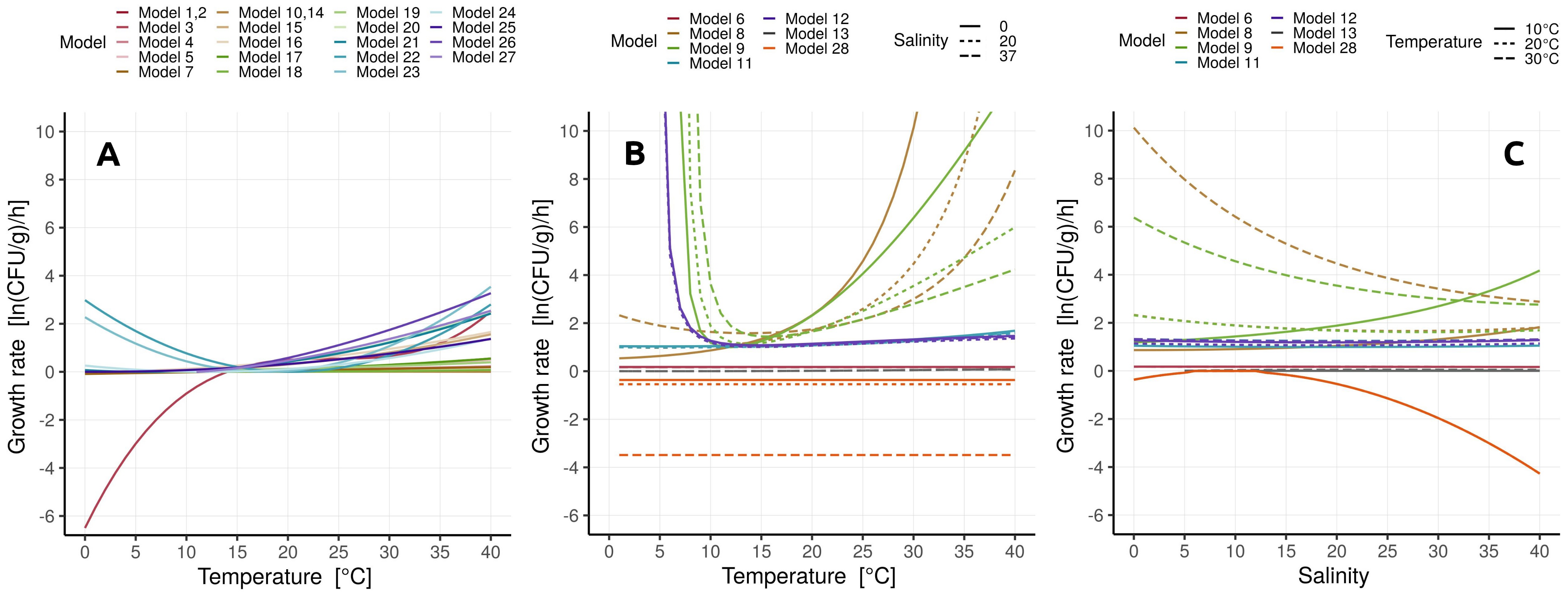
3.1. Vibrio spp. Growth Models

Vibrio spp. growth models identified by the literature review could be partitioned into 12 primary (Table 1) and 8 secondary (Table 2) models, using the parameters listed in Table 3. In total, we identified 29 models for Vibrio spp. growth in a dynamic environment, but we could not find parameter values for Fujikawa et al. [50]. Therefore, we further analyzed only the remaining 28 models (Table 4), using the parameters listed in Table A1.

The model summaries (Table 4) provide an overview of the models used when studying Vibrio spp. growth in a dynamic environment. The main findings were as follows:

• Baranyi and modified Gompertz are the most commonly used primary models for describing Vibrio spp. growth over time.
• Square root and Arrhenius-based models are the most frequently applied secondary models for Vibrio spp. growth in dynamic conditions.
• V. cholerae, V. parahaemolyticus, V. harveyi, and V. vulnificus are the species used most often as modeling organisms.
• Vibrio growth was monitored in/on various substrates (free water column, within organisms, in broth substrates, etc.), under different temperature, salinity, and pH conditions. This implies that the aquatic environments and organisms (marine and freshwater), as well as food and water health and safety, are the key areas of research and concern.
• Temperature was the prevailing environmental parameter used in secondary models, implying a strong effect of temperature on Vibrio spp. abundance. The effect of temperature on the primary model parameters (growth rate and lag time) was most often modeled by the square root or the Arrhenius-based model.

3.2. Vibrio In Situ Datasets

We summarize the dataset classification and characteristics of the seven datasets in Table 5, including the number of Vibrio spp. abundance data, and range and type of environmental variables used in model validation (temperature, salinity, pH). Datasets URB2 and COAST do not contain information on pH, so simulations of Model 6 (Table 4) were not possible for those datasets.

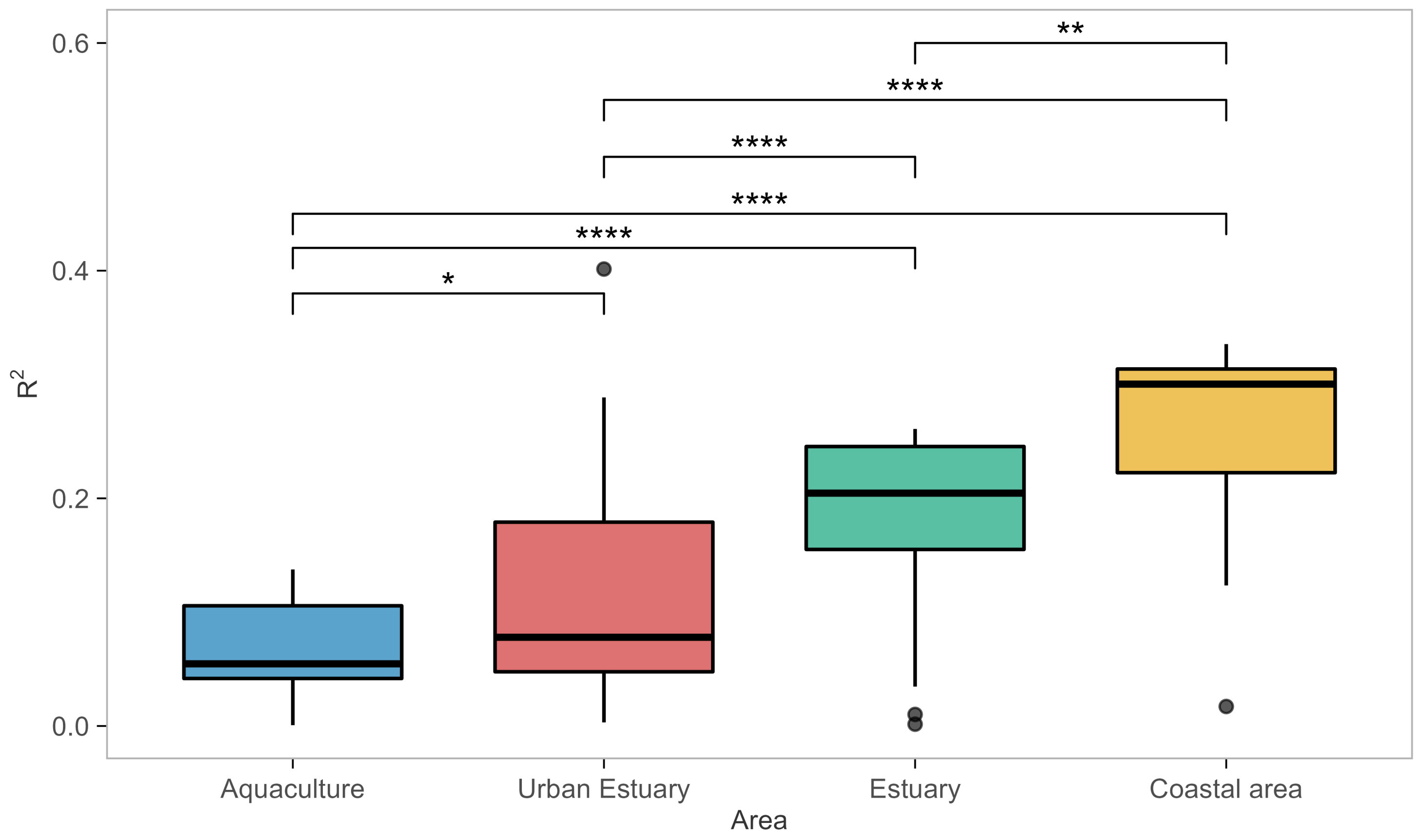
3.3. Model Performance

The ability of models to describe the data greatly varied between models and datasets (Figure 2). The calculated $R^2$ values ranged from <0.001 (Model 10 for dataset AQC1) to 0.40 (Model 28, dataset URB2), with the overall median value of all models for all datasets $R^2=0.13$. $R^2$ values also significantly differed between habitat types (Figure 3,

Table A2. Results of robust ANOVA one-way test from the package WRS2 [61].

Function:	t1way (formula = max_r2~Habitat, data = as)
Test statistic:	F = 75.561
Degrees of freedom 1:	3
Degrees of freedom 2:	49.90
p-value:	0
Explanatory measure of effect size:	0.77
Bootstrap CI:	[0.68; 0.84]

) in all pairwise comparisons (post hoc tests p < 0.017; see details in

Table A3. Results of post hoc lincon test from the package WRS2 [61].

Formula:		lincon (max_r2~Habitat, data = as)
Habitat type	psihat	ci.lower	ci. upper	p-value
Aquaculture vs. Urban Estuary	−0.03910	−0.08237	0.00417	0.01688
Aquaculture vs. Estuary	−0.14203	−0.17331	−0.11075	0.00000
Aquaculture vs. Coastal Area	−0.21525	−0.27062	−0.15989	0.00000
Urban Estuary vs. Estuary	−0.10293	−0.14925	−0.05662	0.00000
Urban Estuary vs. Coastal Area	−0.17616	−0.23977	−0.11254	0.00000
Estuary vs. Coastal Area	−0.07322	−0.13069	−0.01575	0.00263

). Therefore, $R^2$ values suggest the models performed best for coastal areas, followed by estuaries, urban estuaries, and aquaculture habitats. Comparing $R^2$ values provides performance estimates of a particular model on a particular dataset, but does not provide information on generality.

Model generality analysis (Figure 4A) shows rankings above the median ($R^2>0.13$) where:

• All models except Model 6 (Baranyi with polinomial pH and salinity secondary models) were able to score above average at least in some habitats, i.e., capture those habitats. Incidentally, Model 6 was the only one not applying a temperature correction
• A total of 93% of models captured the coastal area habitat.
• A total of 93% of all models captured estuary habitat, but only 85% of those (i.e., 79% of all models) captured both estuary datasets; 26 models captured EST1, with 22 of them capturing EST2 as well.
• A total of 75% of models captured an urban habitat, but only two (Models 9 and 28) captured both urban habitat datasets; URB1 was captured by all 20 of them; only 3 models managed to capture URB2.
• Only the Baranyi-type model (Model 8, with temperature and salinity secondary models) captured the AQC1 aquaculture habitat.
• The model with the highest $R^2$ values (Model 28—net exponential, for urban estuary URB2) had low generality, as it captured datasets from only two out of four habitats.
• Of the models that performed well for at least one habitat type, Model 17 had lowest generality as it captured only one EST1 dataset.

Selecting for better capability by scoring only performances within the first quartile ($R^2>0.22$, Figure 4B) shows that:

• ≈A total of 72% of the analyzed models had an exceptional ability to capture datasets from the coastal area habitat.
• The ability of models to capture/perform well for estuarine habitats was severely diminished, with only 16/28 (57% of the models) capturing one of the two estuary datasets, and only 10 models (36%) capturing both.
• None of the models were able to capture for the aquaculture habitat datasets, and only three (Models 8, 9, and 28) captured the urban estuary habitat.
• Model 28 seemed even more specialized, as it captured a single urban estuary (URB2)
• Most prolific Baranyi models (Models 8 and 9) remained so by capturing datasets from three habitat types, albeit only a single dataset from each.

4. Discussion

Our work adds to the growing body of knowledge from the past few decades that helped refine a general understanding of the ecology of Vibrio spp. We (i) summarized dynamics and unified nomenclature for all published functional models we could find (12 primary and 8 secondary), (ii) added two datasets to the existing five longitudinal datasets on Vibrio spp. and their environments, and (iii) used the datasets to asses the ability of existing models to capture Vibrio spp. abundances in four different habitat types.

There are no clear winners between the 28 investigated models. Generally, the $R^2$ values were not particularly large (≤0.40), but the values can be considered acceptable given the difficulty of the task, in particular the multitude of potential factors affecting both the environment and the Vibrio populations.

Baranyi-based models (Models 2 to 10 in Table 4) seemed to capture the widest variety of habitats well, with Models 8 and 9 leading the way in diversity. Although both models had a similar $R^2$ for the AQC1 dataset (0.14 and 0.12, respectively), Model 8 was the only one that crossed the median threshold and therefore captured an aquaculture dataset as an above-average performer. Notably, Models 8 and 9 are the only Baranyi-based models that included both temperature and salinity secondary models. Model 28 (net exponential) also included both factors and performed quite well, giving the highest overall $R^2$ (0.40 for the URB2 dataset).

Inclusion of temperature and salinity, however, does not guarantee success. All three Gompertz-based models included both factors, but all three underperformed. This would signal Gompertz-based models should be used with caution. Modified Gompertz-based models (Models 14–24), however, seem to lag only slightly behind the best.

While it may be tempting to proclaim Baranyi-based models as the most versatile, they do have significant drawbacks. First, both Models 8 and 9 had issues with simulations: their fast growth rate sometimes caused very large predictions (see Appendix D). While this has not been a problem for the optimal run time of Model 8, Model 9 did lose up to 3% of data in the evaluation. These issues may not be consequential in the current assessment, but may become so in new datasets.

Second, the secondary models accounting for salinity in Models 8 and 9 yielded unexpected growth rate patterns. For example, at moderate and high salinities, growth rates could be extremely high at the ends of the environmental temperature range (e.g., 3.18 ln(CFU/g)/h for salinity of 20 and temperature of 27 °C, Figure 5, Panel B). Likewise, at 10 °C, the growth rate of Model 8 was moderate and slightly increased with salinity; at 30 °C, however, the rate was extremely high for low salinity, and rapidly decreased with salinity. This may be plausible as abundance of Vibrio spp. increased with water temperatures during periods of reduced salinity [73], but we recommend caution when utilizing Baranyi-based models in highly variable environments.

Overall, predictions for the coastal area and estuary datasets seemed to be more robust than those for urban estuaries and aquaculture (Figure 4, Panel B). We hypothesize this may be due to higher levels of anthropogenic disturbance in aquaculture and urban estuaries, in particular potentially high inputs of organic matter. Vibrio spp., as a prototypical copiotroph, dominates in nutrient-rich environments [74]. They exhibit a feast-and-famine lifestyle and swim to colonize sporadic, nutrient-rich patches and particles [75]. Therefore, we think that organic matter has an important role in determining Vibrio spp. abundance, especially in these types of habitats.

Our study has some limitations. First, we treated all Vibrio spp. the same. While justified in the context of a wide assessment such as ours, Vibrio species clearly differ and could potentially exhibit significantly different dynamics, especially since different species favor different environmental conditions. These differences could become important as environmental conditions change, and the Vibrio community could shift towards disease-causing species. Unfortunately, current datasets and available models do not allow for a deeper investigation of the issue.

Second, we chose the simulation time that minimized $R^2$, but relied on a single simulation time for each dataset. In principle, a different simulation time could be chosen for each data point. Such an approach would, however, in effect result in fitting each value by choosing simulation time that gives a desired result, thus defeating the purpose of modeling. There could, nonetheless, be some value in exploring functional dependencies of the simulation time on various environmental factors (temperature in particular), but additional research would be required to suggest a particular form of such a function.

Third, we set out to investigate published parameters and models with well-defined functional forms. Perhaps a different set of parameters and/or combinations of models could have described the datasets better. We have made a first step towards such research by systematizing primary and secondary models, parameters, and available—including two previously unpublished—datasets. Alternatively, statistical models could possibly be re-fitted to better capture the datasets. Such statistical approaches may be appropriate in some cases, e.g., when aiming to inter- or extrapolate data from a single area.

Clearly, additional research is needed for developing a growth model capable of predicting in situ Vibrio spp. abundances in natural environments. We suggest further development of secondary models should be one priority; dynamics of secondary models should be well-defined for the whole range of expected environmental factors, especially temperature and salinity. Modeling could also benefit from research on additional environmental factors such as organic matter, which has been shown to affect Vibrio growth [56]. Given the role of Vibrio spp. in aquatic environments, it is surprising that less than half datasets include organic matter measurements. We suggest that future modeling development should include organic matter, especially when sampling to ensure measurement of organic matter.

Perhaps a development of a third generation of models based on big data and deep learning could also work in synergy with mechanistic modeling to improve our ability to predict Vibrio spp. dynamics in a changing environment. Improved models could then enhance predictive frameworks, e.g., by replacing the basic ecological niche approach to estimating Vibrio presence used in exploration of future risk scenarios by Trinanes and Martinez-Urtaza [76].

In conclusion, none of the investigated models provide a complete solution: Baranyi-based models might be the most versatile, but other models (e.g., net exponential) may provide a better fit for a particular cause. Therefore, the choice of the model should be at least in part guided by the type of the environment and expected ranges of environmental factors; if many data lie outside of the well-described range of a particular secondary model (see Figure 5), perhaps a different model should be tried instead. Our summary and systematization (Table 1, Table 2, Table 3, Table 4 and Table 5) provide currently available primary and secondary models, and data, which can be used as a toolbox for model creation and testing.

References

1. Zhang, X.; Lin, H.; Wang, X.; Austin, B. Significance of Vibrio species in the marine organic carbon cycle—A review. Sci. China Earth Sci. 2018, 61, 1357–1368. [Google Scholar] [CrossRef]
2. Sampaio, A.; Silva, V.; Poeta, P.; Aonofriesei, F. Vibrio spp.: Life strategies, ecology, and risks in a changing environment. Diversity 2022, 14, 97. [Google Scholar] [CrossRef]
3. Thompson, J.R.; Polz, M.F. Dynamics of Vibrio populations and their role in environmental nutrient cycling. In The Biology of Vibrios; Wiley Online Library: Hoboken, NJ, USA, 2006; pp. 190–203. [Google Scholar]
4. Beardsley, C.; Pernthaler, J.; Wosniok, W.; Amann, R. Are readily culturable bacteria in coastal North Sea waters suppressed by selective grazing mortality? Appl. Environ. Microbiol. 2003, 69, 2624–2630. [Google Scholar] [CrossRef] [PubMed]
5. Ganesan, D.; Gupta, S.S.; Legros, D. Cholera surveillance and estimation of burden of cholera. Vaccine 2020, 38, A13–A17. [Google Scholar] [CrossRef]
6. Gilbert, J.A.; Steele, J.A.; Caporaso, J.G.; Steinbrück, L.; Reeder, J.; Temperton, B.; Huse, S.; McHardy, A.C.; Knight, R.; Joint, I.; et al. Defining seasonal marine microbial community dynamics. ISME J. 2012, 6, 298–308. [Google Scholar] [CrossRef]
7. Westrich, J.R.; Ebling, A.M.; Landing, W.M.; Joyner, J.L.; Kemp, K.M.; Griffin, D.W.; Lipp, E.K. Saharan dust nutrients promote Vibrio bloom formation in marine surface waters. Proc. Natl. Acad. Sci. USA 2016, 113, 5964–5969. [Google Scholar] [CrossRef]
8. Poloczanska, E.S.; Brown, C.J.; Sydeman, W.J.; Kiessling, W.; Schoeman, D.S.; Moore, P.J.; Brander, K.; Bruno, J.F.; Buckley, L.B.; Burrows, M.T.; et al. Global imprint of climate change on marine life. Nat. Clim. Chang. 2013, 3, 919–925. [Google Scholar] [CrossRef]
9. Dore, M.H. Climate change and changes in global precipitation patterns: What do we know? Environ. Int. 2005, 31, 1167–1181. [Google Scholar] [CrossRef]
10. Bijma, J.; Pörtner, H.O.; Yesson, C.; Rogers, A.D. Climate change and the oceans—What does the future hold? Mar. Pollut. Bull. 2013, 74, 495–505. [Google Scholar] [CrossRef]
11. Burge, C.A.; Hershberger, P.K. Climate change can drive marine diseases. In Marine Disease Ecology; Behringer, D.C., Silliman, B.R., Lafferty, K.D., Eds.; Oxford University Press: Oxford, UK, 2020; pp. 83–94. [Google Scholar]
12. Martinez-Urtaza, J.; Bowers, J.C.; Trinanes, J.; DePaola, A. Climate anomalies and the increasing risk of Vibrio parahaemolyticus and Vibrio vulnificus illnesses. Food Res. Int. 2010, 43, 1780–1790. [Google Scholar] [CrossRef]
13. Da Cunha, D.T. Improving food safety practices in the foodservice industry. Curr. Opin. Food Sci. 2021, 42, 127–133. [Google Scholar] [CrossRef]
14. Levallois, P.; Villanueva, C.M. Drinking water quality and human health: An editorial. Int. J. Environ. Res. Public Health 2019, 16, 631. [Google Scholar] [CrossRef]
15. Li, H.; Xie, G.; Edmondson, A.S. Review of secondary mathematical models of predictive microbiology. J. Food Prod. Mark. 2008, 14, 57–74. [Google Scholar] [CrossRef]
16. Ferrer, J.; Prats, C.; López, D.; Vives-Rego, J. Mathematical modeling methodologies in predictive food microbiology: A SWOT analysis. Int. J. Food Microbiol. 2009, 134, 2–8. [Google Scholar] [CrossRef]
17. Peleg, M.; Corradini, M.G. Microbial growth curves: What the models tell us and what they cannot. Crit. Rev. Food Sci. Nutr. 2011, 51, 917–945. [Google Scholar] [CrossRef]
18. Perez-Rodriguez, F.; Valero, A. Predictive microbiology in foods. In Predictive Microbiology in Foods; Springer: Berlin/Heidelberg, Germany, 2013; pp. 1–10. [Google Scholar]
19. Oscar, T. Development and validation of primary, secondary, and tertiary models for growth of Salmonella Typhimurium on sterile chicken. J. Food Prot. 2005, 68, 2606–2613. [Google Scholar] [CrossRef]
20. Baranyi, J.; McClure, P.; Sutherland, J.; Roberts, T. Modeling bacterial growth responses. J. Ind. Microbiol. Biotechnol. 1993, 12, 190–194. [Google Scholar] [CrossRef]
21. Pirt, S.J. Principles of Microbe and Cell Cultivation; Blackwell Scientific Publications: Hoboken, NJ, USA, 1975. [Google Scholar]
22. Ratkowsky, D.; Lowry, R.; McMeekin, T.; Stokes, A.; Chandler, R. Model for bacterial culture growth rate throughout the entire biokinetic temperature range. J. Bacteriol. 1983, 154, 1222–1226. [Google Scholar] [CrossRef]
23. Davey, K. A predictive model for combined temperature and water activity on microbial growth during the growth phase. J. Appl. Bacteriol. 1989, 67, 483–488. [Google Scholar] [CrossRef]
24. Esser, D.S.; Leveau, J.H.; Meyer, K.M. Modeling microbial growth and dynamics. Appl. Microbiol. Biotechnol. 2015, 99, 8831–8846. [Google Scholar] [CrossRef]
25. Zwietering, M.; Jongenburger, I.; Rombouts, F.; Van’t Riet, K. Modeling of the bacterial growth curve. Appl. Environ. Microbiol. 1990, 56, 1875–1881. [Google Scholar] [CrossRef] [PubMed]
26. Fu, S.; Shen, J.; Liu, Y.; Chen, K. A predictive model of V ibrio cholerae for combined temperature and organic nutrient in aquatic environments. J. Appl. Microbiol. 2013, 114, 574–585. [Google Scholar] [CrossRef]
27. Fu, S.; Liu, Y.; Li, X.; Tu, J.; Lan, R.; Tian, H. A preliminary stochastic model for managing microorganisms in a recirculating aquaculture system. Ann. Microbiol. 2015, 65, 1119–1129. [Google Scholar] [CrossRef]
28. Ma, F.; Liu, H.; Wang, J.; Zhang, Z.; Sun, X.; Pan, Y.; Zhao, Y. Behavior of Vibrio parahemolyticus cocktail including pathogenic and nonpathogenic strains on cooked shrimp. Food Control 2016, 68, 124–132. [Google Scholar] [CrossRef]
29. Zahaba, M.; Halmi, M.I.E.; Othman, A.R.; Shukor, M.Y. Mathematical modeling of the growth curve of Vibrio sp. isolate MZ grown in Seawater medium. Bioremediation Sci. Technol. Res. 2018, 6, 31–34. [Google Scholar] [CrossRef]
30. Baranyi, J.; Roberts, T.A. Mathematics of predictive food microbiology. Int. J. Food Microbiol. 1995, 26, 199–218. [Google Scholar] [CrossRef]
31. Boonyawantang, A.; Mahakarnchanakul, W.; Rachtanapun, C.; Boonsupthip, W. Behavior of pathogenic Vibrio parahaemolyticus in prawn in response to temperature in laboratory and factory. Food Control 2012, 26, 479–485. [Google Scholar] [CrossRef]
32. Chung, K.H.; Park, M.S.; Kim, H.Y.; Bahk, G.J. Growth prediction and time–temperature criteria model of Vibrio parahaemolyticus on traditional Korean raw crab marinated in soy sauce (ganjang-gejang) at different storage temperatures. Food Control 2019, 98, 187–193. [Google Scholar] [CrossRef]
33. Fernandez-Piquer, J.; Bowman, J.P.; Ross, T.; Tamplin, M.L. Predictive models for the effect of storage temperature on Vibrio parahaemolyticus viability and counts of total viable bacteria in Pacific oysters (Crassostrea gigas). Appl. Environ. Microbiol. 2011, 77, 8687–8695. [Google Scholar] [CrossRef] [PubMed]
34. Oh, H.; Yoon, Y.; Ha, J.; Lee, J.; Shin, I.S.; Kim, Y.M.; Park, K.S.; Kim, S. Risk assessment of vibriosis by Vibrio cholerae and Vibrio vulnificus in whip-arm octopus consumption in South Korea. Fish. Aquat. Sci. 2021, 24, 207–218. [Google Scholar] [CrossRef]
35. Parveen, S.; DaSilva, L.; DePaola, A.; Bowers, J.; White, C.; Munasinghe, K.A.; Brohawn, K.; Mudoh, M.; Tamplin, M. Development and validation of a predictive model for the growth of Vibrio parahaemolyticus in post-harvest shellstock oysters. Int. J. Food Microbiol. 2013, 161, 1–6. [Google Scholar] [CrossRef]
36. Posada-Izquierdo, G.D.; Valero, A.; Arroyo-López, F.N.; González-Serrano, M.; Ramos-Benítez, A.M.; Benítez-Cabello, A.; Rodríguez-Gómez, F.; Jimenez-Diaz, R.; García-Gimeno, R.M. Behavior of Vibrio spp. in table olives. Front. Microbiol. 2021, 2021, 1130. [Google Scholar] [CrossRef]
37. Zhou, K.; Gui, M.; Li, P.; Xing, S.; Cui, T.; Peng, Z. Effect of combined function of temperature and water activity on the growth of Vibrio harveyi. Braz. J. Microbiol. 2012, 43, 1365–1375. [Google Scholar] [CrossRef]
38. Miles, D.W.; Ross, T.; Olley, J.; McMeekin, T.A. Development and evaluation of a predictive model for the effect of temperature and water activity on the growth rate of Vibrio parahaemolyticus. Int. J. Food Microbiol. 1997, 38, 133–142. [Google Scholar] [CrossRef]
39. Nishina, T.; Wada, M.; Ozawa, H.; Hara-Kudo, Y.; Konuma, H.; Hasegawa, J.; Kumagi, S. Growth kinetics of Vibrio parahaemolyticus O3: K6 under varying conditions of pH, NaCl concentration and temperature. Food Hyg. Saf. Sci. 2004, 45, 35–37. [Google Scholar] [CrossRef]
40. Kim, Y.W.; Lee, S.H.; Hwang, I.G.; Yoon, K.S. Effect of temperature on growth of Vibrio paraphemolyticus and Vibrio vulnificus in flounder, salmon sashimi and oyster meat. Int. J. Environ. Res. Public Health 2012, 9, 4662–4675. [Google Scholar] [CrossRef]
41. Yang, Z.Q.; Jiao, X.A.; Li, P.; Pan, Z.M.; Huang, J.L.; Gu, R.X.; Fang, W.M.; Chao, G.X. Predictive model of Vibrio parahaemolyticus growth and survival on salmon meat as a function of temperature. Food Microbiol. 2009, 26, 606–614. [Google Scholar] [CrossRef]
42. Yoon, K.; Min, K.; Jung, Y.; Kwon, K.; Lee, J.; Oh, S. A model of the effect of temperature on the growth of pathogenic and nonpathogenic Vibrio parahaemolyticus isolated from oysters in Korea. Food Microbiol. 2008, 25, 635–641. [Google Scholar] [CrossRef]
43. Van Boekel, M.A. On the use of the Weibull model to describe thermal inactivation of microbial vegetative cells. Int. J. Food Microbiol. 2002, 74, 139–159. [Google Scholar] [CrossRef]
44. Buchanan, R.; Whiting, R.; Damert, W. When is simple good enough: A comparison of the Gompertz, Baranyi, and three-phase linear models for fitting bacterial growth curves. Food Microbiol. 1997, 14, 313–326. [Google Scholar] [CrossRef]
45. Tang, X.; Zhao, Y.; Sun, X.; Xie, J.; Pan, Y.; Malakar, P.K. Predictive model of Vibrio parahaemolyticus O3: K6 growth on cooked Litopenaeus vannamei. Ann. Microbiol. 2015, 65, 487–493. [Google Scholar]
46. Huang, L. Growth kinetics of Listeria monocytogenes in broth and beef frankfurters—Determination of lag phase duration and exponential growth rate under isothermal conditions. J. Food Sci. 2008, 73, E235–E242. [Google Scholar] [CrossRef] [PubMed]
47. Chen, Y.R.; Hwang, C.A.; Huang, L.; Wu, V.C.; Hsiao, H.I. Kinetic analysis and dynamic prediction of growth of vibrio parahaemolyticus in raw white shrimp at refrigerated and abuse temperatures. Food Control 2019, 100, 204–211. [Google Scholar] [CrossRef]
48. Fang, T.; Gurtler, J.B.; Huang, L. Growth kinetics and model comparison of Cronobacter sakazakii in reconstituted powdered infant formula. J. Food Sci. 2012, 77, E247–E255. [Google Scholar] [CrossRef] [PubMed]
49. Froelich, B.; Bowen, J.; Gonzalez, R.; Snedeker, A.; Noble, R. Mechanistic and statistical models of total Vibrio abundance in the Neuse River Estuary. Water Res. 2013, 47, 5783–5793. [Google Scholar] [CrossRef]
50. Fujikawa, H.; Kai, A.; Morozumi, S. A new logistic model for bacterial growth. Shokuhin Eiseigaku Zasshi. J. Food Hyg. Soc. Jpn. 2003, 44, 155–160. [Google Scholar] [CrossRef] [PubMed]
51. Fujikawa, H. Application of the new logistic model to microbial growth prediction in food. Biocontrol Sci. 2011, 16, 47–54. [Google Scholar] [CrossRef]
52. Ratkowsky, D.A.; Olley, J.; McMeekin, T.; Ball, A. Relationship between temperature and growth rate of bacterial cultures. J. Bacteriol. 1982, 149, 1–5. [Google Scholar] [CrossRef]
53. Huang, L.; Hwang, C.A.; Phillips, J. Evaluating the Effect of Temperature on Microbial Growth Rate—The Ratkowsky and a Bělehrádek-Type Models. J. Food Sci. 2011, 76, M547–M557. [Google Scholar] [CrossRef]
54. Kapetanović, D.; Purgar, M.; Gavrilović, A.; Hackenberger, B.K.; Kurtović, B.; Haberle, I.; Pečar Ilić, J.; Geček, S.; Hackenberger, D.K.; Djerdj, T.; et al. AqADAPT: Physiochemical parameters and Vibrio spp. abundance in water samples gathered in the Adriatic Sea. PANGAEA 2022. submitted. [Google Scholar]
55. Jug-Dujaković, J.; Gavrilović, A.; Kolda, A.; Žunić, J.; Pikelj, K.; Listeš, E.; Vukić Lušić, D.; Vardić Smrzlić, L.; Perić, L.; El-Matbouli, M.; et al. AQUAHEALTH: Physiochemical parameters and Vibrio spp. abundance in water samples gathered in the Adriatic Sea. PANGAEA 2022. submitted. [Google Scholar]
56. Bullington, J.A.; Golder, A.R.; Steward, G.F.; McManus, M.A.; Neuheimer, A.B.; Glazer, B.T.; Nigro, O.D.; Nelson, C.E. Refining real-time predictions of Vibrio vulnificus concentrations in a tropical urban estuary by incorporating dissolved organic matter dynamics. Sci. Total Environ. 2022, 829, 154075. [Google Scholar] [CrossRef] [PubMed]
57. Nigro, O.D.; James-Davis, L.I.; De Carlo, E.H.; Li, Y.H.; Steward, G.F. Variable freshwater influences on the abundance of Vibrio vulnificus in a tropical urban estuary. Appl. Environ. Microbiol. 2022, 88, e01884-21. [Google Scholar] [CrossRef] [PubMed]
58. Froelich, B.; Gonzalez, R.; Blackwood, D.; Lauer, K.; Noble, R. Decadal monitoring reveals an increase in Vibrio spp. concentrations in the Neuse River Estuary, North Carolina, USA. PLoS ONE 2019, 14, e0215254. [Google Scholar] [CrossRef]
59. Urquhart, E.A.; Jones, S.H.; Yu, J.W.; Schuster, B.M.; Marcinkiewicz, A.L.; Whistler, C.A.; Cooper, V.S. Environmental conditions associated with elevated Vibrio parahaemolyticus concentrations in Great Bay Estuary, New Hampshire. PLoS ONE 2016, 11, e0155018. [Google Scholar] [CrossRef]
60. Williams, T.C.; Froelich, B.A.; Phippen, B.; Fowler, P.; Noble, R.T.; Oliver, J.D. Different abundance and correlational patterns exist between total and presumed pathogenic Vibrio vulnificus and V. parahaemolyticus in shellfish and waters along the North Carolina coast. FEMS Microbiol. Ecol. 2017, 93, 71. [Google Scholar] [CrossRef] [PubMed]
61. Mair, P.; Wilcox, R. Robust statistical methods in R using the WRS2 package. Behav. Res. Methods 2020, 52, 464–488. [Google Scholar] [CrossRef]
62. Wilcox, R.R. Introduction to Robust Estimation and Hypothesis Testing, 3rd ed.; Elsevier: Amsterdam, The Netherlands, 2012. [Google Scholar]
63. RStudio Team. RStudio: Integrated Development Environment for R; RStudio, PBC: Boston, MA, USA, 2020. [Google Scholar]
64. Wickham, H.; Averick, M.; Bryan, J.; Chang, W.; McGowan, L.D.; François, R.; Grolemund, G.; Hayes, A.; Henry, L.; Hester, J.; et al. Welcome to the tidyverse. J. Open Source Softw. 2019, 4, 1686. [Google Scholar] [CrossRef]
65. Kuhn, M. Building Predictive Models in R Using the caret Package. J. Stat. Software Artic. 2008, 28, 1–26. [Google Scholar] [CrossRef]
66. Hamner, B.; Frasco, M.; LeDell, E. Evaluation Metrics for Machine Learning. 2018. Available online: https://cran.r-project.org/web/packages/Metrics/Metrics.pdf (accessed on 25 April 2022).
67. Grosjean, P. SciViews–Main Package. 2019. Available online: https://cran.r-project.org/web/packages/SciViews/SciViews.pdf (accessed on 25 April 2022).
68. Dowle, M. Package ‘data.table’: Extension of ‘data.frame’. 2021. Available online: https://cran.r-project.org/web/packages/data.table/data.table.pdf (accessed on 25 April 2022).
69. Wickham, H. Read Excel Files. 2019. Available online: https://cran.microsoft.com/snapshot/2019-03-09/web/packages/readxl/readxl.pdf (accessed on 25 April 2022).
70. Dragulescu, A.; Arendt, C. Read, Write, Format Excel 2007 and Excel 97/2000/XP/2003 Files. 2020. Available online: https://cran.r-project.org/web/packages/xlsx/xlsx.pdf (accessed on 25 April 2022).
71. Purgar, M.; Kapetanović, D.; Geček, S.; Marn, N.; Haberle, I.; Hackenberger, K.B.; Gavrilović, A.; Pečar Ilić, J.; Hackenberger K., D.; Djerdj, T.; et al. Codes for Purgar et al. 2022: Investigating the ability of growth models to predict in situ Vibrio spp. abundances. Zenodo 2022. [Google Scholar] [CrossRef]
72. Wickham, H. ggplot2: Elegant Graphics for Data Analysis; Springer: New York, NY, USA, 2016. [Google Scholar]
73. Martinez-Urtaza, J.; Lozano-Leon, A.; Varela-Pet, J.; Trinanes, J.; Pazos, Y.; Garcia-Martin, O. Environmental determinants of the occurrence and distribution of Vibrio parahaemolyticus in the rias of Galicia, Spain. Appl. Environ. Microbiol. 2008, 74, 265–274. [Google Scholar] [CrossRef]
74. Kirchman, D.L. Growth rates of microbes in the oceans. Annu. Rev. Mar. Sci. 2016, 8, 285–309. [Google Scholar] [CrossRef]
75. Norris, N.; Levine, N.M.; Fernandez, V.I.; Stocker, R. Mechanistic model of nutrient uptake explains dichotomy between marine oligotrophic and copiotrophic bacteria. PLoS Comput. Biol. 2021, 17, e1009023. [Google Scholar] [CrossRef]
76. Trinanes, J.; Martinez-Urtaza, J. Future scenarios of risk of Vibrio infections in a warming planet: A global mapping study. Lancet Planet. Health 2021, 5, e426–e435. [Google Scholar] [CrossRef]
77. Ouzzani, M.; Hammady, H.; Fedorowicz, Z.; Elmagarmid, A. Rayyan—A web and mobile app for systematic reviews. Syst. Rev. 2016, 5, 1–10. [Google Scholar] [CrossRef]
78. Gekas, V.; Gonzalez, C.; Sereno, A.; Chiralt, A.; Fito, P. Mass transfer properties of osmotic solutions. I. Water activity and osmotic pressure. Int. J. Food Prop. 1998, 1, 95–112. [Google Scholar] [CrossRef] [Green Version]
Figure 1. The methodological approach to model analysis. We performed a literature search to find all Vibrio spp. growth models and all available datasets suitable for comparison. We found five published datasets, and included two of our own collected through projects AqADAPT and AQUAHEALTH of the Croatian Science Foundation (HRZZ).
Microorganisms 10 01765 g001
Figure 2. R2 calculated for all models and for each dataset. Horizontal line depicts the median R 2 = 0.13 used to evaluate model performance. Primary models are labeled as follows: ML—modified logistic, Baranyi, Gompertz, modified Gompertz, TPL—three-phase linear, HPM—Huang primary, NL—no-lag and NE—net exponential. Star (*) signifies models that had an evaluation issue with some of the data points in some of the datasets (details in Appendix D).
Microorganisms 10 01765 g002
Figure 3. Boxplot of model performance measured as R 2 in different habitat types (as classified in Table 5). Model performance significantly differed between habitat types (robust ANOVA, F(3,75.561) = 49.9, p < 0.001, effect size ξ = 0.77, confidence interval CI( ξ ) = [0.68, 0.84]; Table A2). Significance codes are as follows: p 0 ‘****’, p < 0.01 ‘**’, and p < 0.5 ‘*’.
Microorganisms 10 01765 g003
Figure 4. Model generality. Stacked bar chart used for graphical representation of model’s applicability on the dataset from a specific habitat: colors represent habitats (see the legend), and stars (*) denote models that exhibit the evaluation issue with some of the data points in some of the datasets (details in Appendix D). Values on y axis denote the frequency of occurrence of a particular model whose R2 value is above the median ( R 2 > 0.13 ; Panel A), and in the first quartile ( R 2 > 0.22 ; Panel B). Primary models are labeled as follows: ML—modified logistic, Baranyi, Gompertz, modified Gompertz, TPL—three-phase linear, HPM—Huang primary, NL—no-lag and NE—net exponential. Star (*) signifies models that had an evaluation issue with some of the data points in some of the datasets (details in Appendix D). Note that there is only one coastal area dataset, while other habitats have two datasets each. Hence, scoring a single occurrence of the coastal area habitat represents a 100% success rate, while scoring the same in any other habitat represents a success rate of 50%.
Microorganisms 10 01765 g004
Figure 5. Relationships between growth rate and environmental variables as predicted by secondary models. The models in panel (A) include only a temperature correction. Panel (B) shows dependence of growth rate on temperature for three salinity levels. Panel (C) shows dependence of growth rate on salinity for three temperatures. A pH value of 8.1 was assumed for Model 6. Model 28 had a flat temperature response because it used the default parameter value [49] that minimized temperature correction, θ = 1 ; increasing θ would increase the temperature dependence.
Microorganisms 10 01765 g005