Article

Compound Fault Diagnosis and Sequential Prognosis for Electric Scooter with Uncertainties

1
School of Electrical Engineering and Automation, Hefei University of Technology, Hefei 230009, China
2
College of Science, Health, Engineering and Education, Murdoch University, Perth, WA 6150, Australia
*
Author to whom correspondence should be addressed.
Actuators 2020, 9(4), 128; https://doi.org/10.3390/act9040128
Submission received: 19 October 2020 / Revised: 21 November 2020 / Accepted: 27 November 2020 / Published: 3 December 2020
(This article belongs to the Section Actuators for Land Transport)

Abstract

:
This paper addresses diagnosis and prognosis problems for an electric scooter subjected to parameter uncertainties and compound faults (i.e., permanent fault and intermittent fault with non-monotonic degradation). First, the diagnostic bond graph in linear fractional transformation form is used to model the uncertain electric scooter and derive the analytical redundancy relations incorporating the nominal part and uncertain part, based on which the adaptive thresholds for robust fault detection and the fault signature matrix for fault isolation can be obtained. Second, an adaptive enhanced unscented Kalman filter is proposed to identify the fault magnitudes and distinguish the fault types where an auxiliary detector is introduced to capture the appearing and disappearing moments of intermittent fault. Third, a dynamic model with usage dependent degradation coefficient is developed to describe the degradation process of intermittent fault under various usage conditions. Due to the variation of degradation coefficient and the presence of non-monotonic degradation characteristic under some usage conditions, a sequential prognosis method is proposed where the reactivation of the prognoser is governed by the reactivation events. Finally, the proposed methods are validated by experiment results.

1. Introduction

The electric scooter, also known as mobility scooter, promises to enhance the mobility of older and disabled people. It offers convenience on people’s work and life, but at the same time, brings a security risk, or can even lead to a serious consequence. Therefore, it is imperative to develop a fault diagnosis and prognosis approach to ensure system safety and reliability [1]. Fault diagnosis is an important element of condition-based maintenance and mainly includes fault detection, fault isolation and fault identification [2].
Generally speaking, the faults in monitored systems can be divided into permanent faults and intermittent faults [3]. Abrupt fault and incipient fault are two kinds of well-known permanent faults. To date, fault diagnosis of permanent faults has gained significant attentions and many achievements have been obtained [4]. In [5], a signal-based health monitoring method for gear fault in rotational machine through acoustic emission feature quantification using empirical mode decomposition is proposed. The advantage of this method is that it does not need to build an accurate model for the system under monitoring. One of the problems related to this approach is that some signals in the monitored system cannot be readily obtained. In [6], a bond graph (BG) model-based method is developed for structural component fault detection and isolation (FDI) in intelligent autonomous vehicle using the properties of the bicausality and the causal path. The major advantage of BG is that it can clearly represent causal relations between model variables to deduce the analytical redundancy relations (ARRs) which function as fault indicators. A robust FDI method based on uncertain bond graph (UBG), i.e., diagnostic bond graph in linear fractional transformation (DBG-LFT) form, is proposed in [7] for uncertain systems, where the adaptive threshold is generated to achieve reliable fault detection in the presence of parameter uncertainty. In [8], a robust FDI method for both abrupt and incipient faults in nonlinear uncertain dynamic systems is developed where rigorous analytical results related to the fault isolation time are provided. In [9], a FDI aided fault-tolerant control is introduced for uncertain systems. The controller is reconfigured after FDI to improve the control performance. The main strength of model-based method lies in the fact that it incorporates physical understanding for diagnosis. As a result, this method can achieve better diagnosis performance due to the employment of accurate mathematical model. However, building an accurate mathematical model for complex nonlinear system may not always be a trivial task. In this case, system methods which enable to identify the fault without detailed knowledge of the object under consideration are proposed as alternatives. In [10], a new convolutional neural network based fault diagnosis technique is introduced for fault diagnosis of rotary machines, where the need for manual extraction of features is omitted. Without requirements of fault feature frequency calculations, an identification method using fuzzy clustering for rotational system non-coaxiality is developed in [11].
On the other hand, prognosis of permanent faults aims to predict the end of life (EOL) or remaining useful life (RUL) of a faulty component [12]. Compared with the diagnosis, the prognosis is more efficient in achieving fault prevention, thus prolonging the system lifetime [13]. Due to this property, many works have been done recently in prognosis for a variety of systems [14,15,16,17,18,19,20]. In [14], an artificial intelligence (AI) based method utilizing the fuzzy identification technique is developed. Pająk proposes a model of the operational potential consumption process which uses AI techniques to calculate the change of the operational potential [15]. In [17], a battery health prognosis method for electric vehicles using sample entropy and sparse Bayesian predictive modeling is proposed. The prediction of RUL is realized by integrating sparse Bayesian predictive modeling and bootstrap sampling concepts. In [20], an automatic transmission clutches prognostic scheme is addressed by combining the degradation model with the measurable pre-lockup feature. Note that the above-mentioned prognosis methods are mainly geared towards incipient faults which exhibit degradation trend over time.
Intermittent faults occur randomly with short duration and non-periodically repeated appearance. Since permanent faults will not disappear once they occur, they will not give intermittent symptoms. Intermittent faults are common problems in electronics interconnection systems (wires and connectors), especially for autonomous vehicles, aircrafts, and satellites [21]. Detecting intermittent fault is challenging and frustrating due to its random and unpredictable nature [22]. If these intermittent faults are not handled properly in time, they will degrade over time with increasing frequency, eventually develop into permanent faults. Therefore, it is critical to detect, isolate, and estimate the intermittent faults soon enough such that preventive maintenance can be taken in a timely manner, which ultimately improves the system reliability [23]. In recent years, fault diagnoses of intermittent faults have been widely investigated [21,22,23,24,25,26]. In [24], a chaotic spread spectrum sequence based method is developed for synchronous online diagnosis of intermittent faults in power cables. In this work, the poignant self-correlation characteristic of the chaotic sequences and the cross-correlation characteristics of the chaotic sequences are used to detect single cable intermittent fault and multiple cable intermittent faults, respectively. In [25], a real-time FDI method concerning microsecond intermittent fault based on continuous chaos time-domain reflectometry is proposed for an electrical network. This method not only locates the intermittent fault but also estimates its time of appearance and duration. In [26], an intermittent fault detection method is developed for electronic interconnections by sending a sine wave and decoding the received signal for intermittent information from the channel.
Unlike diagnosis of intermittent fault which is currently an active research field, prognosis of intermittent fault is a new topic where many difficulties are involved. For example, the intermittent fault is discontinuous and non-persistent, existing prognosis methods developed for permanent fault (e.g., incipient fault) with continuous degradation cannot be directly applied. In addition, intermittent faults appear randomly with limited duration, the employed FDI and fault estimation methods (which usually provide valuable information for prognosis, such as true fault and degradation model coefficients [20]) should be able to reliably diagnose the fault as soon as possible. Last but not the least, the degradation trend representing evolution of intermittent fault values at appearing time intervals may be non-monotonic which adds to the difficulty of prognosis algorithm design.
According to aforementioned discussions and findings, it is found that prognosis of intermittent fault is challenging due to its inherent nature (discontinuity, random appearance and disappearance, limited appearing duration, and so on). The situation is further complicated if there is no prior knowledge about fault type (which is the case for practical systems) and the intermittent fault may exhibit non-monotonic characteristic for some usage conditions. This paper attempts to deal with the above difficult issues by developing a BG model-based approach for online fault diagnosis and prognosis of an uncertain electric scooter subjected to compound faults. The main contributions of this work can be summarized as follows:
(1) A single framework, concerning fault diagnosis of both permanent fault and intermittent fault as well as prognosis of intermittent fault in the presence of non-monotonic degradation, is developed for uncertain nonlinear electric scooter system.
(2) An adaptive enhanced unscented Kalman filter (AEUKF) is proposed to distinguish the fault types, track the appearing and disappearing moments of intermittent fault, and adaptively estimate the unknown process noise and measurement noise covariances.
(3) The concept of usage dependent degradation process is developed to describe the degradation trend of intermittent fault, which allows the development of event based sequential prognosis algorithm for intermittent fault in the presence of non-monotonic degradation for certain usage conditions.
This paper is organized as follows: Section 2 describes the detailed UBG model of the electric scooter and introduces the developed FDI approach. In Section 3, the AEUKF-based fault estimation and event based sequential prognosis are presented. In Section 4, experiment results are analyzed in details. Finally, Section 5 concludes the paper.

2. UBG Model and FDI of Electric Scooter

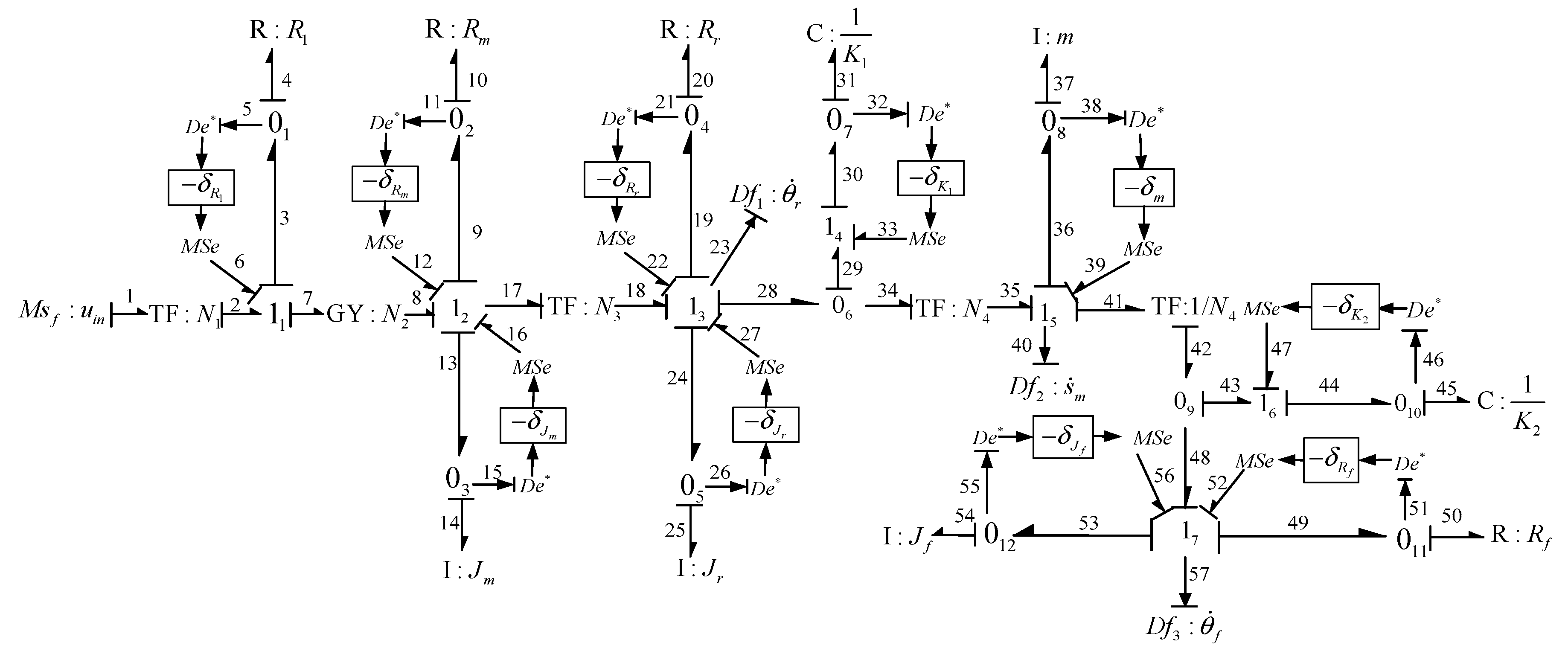
2.1. Electric Scooter System Model
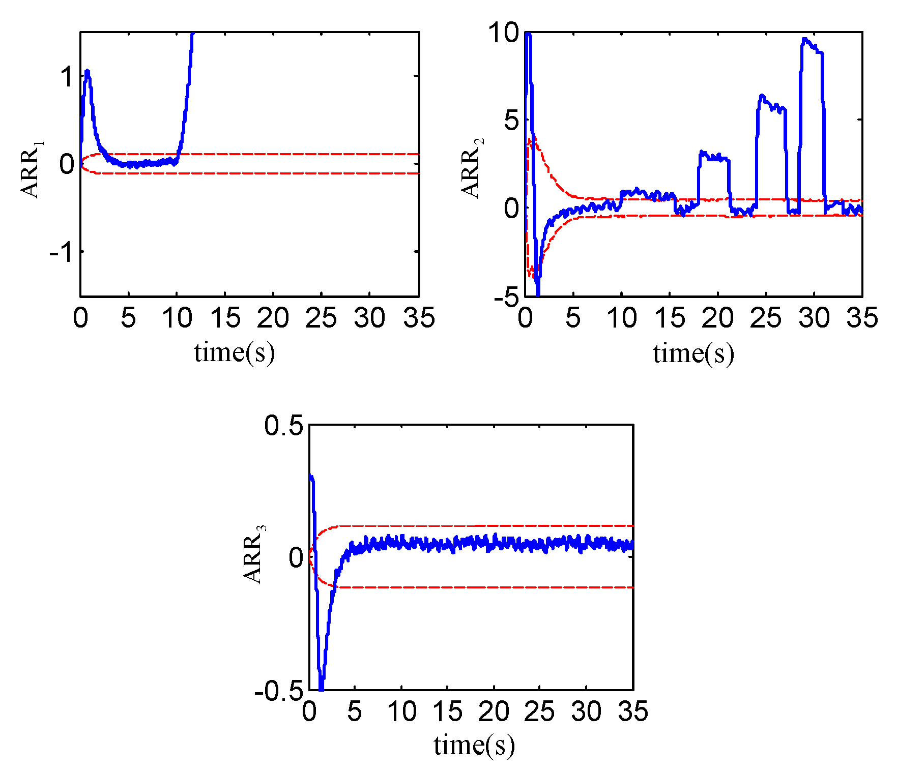
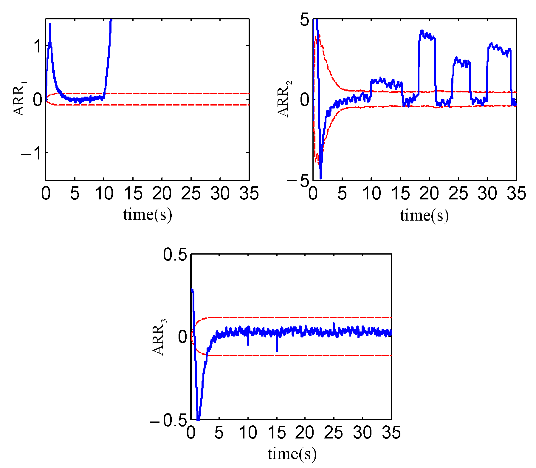
The electric scooter system, as shown in Figure 1, is mainly composed of body, DC motor, motor drive, reducer, and four wheels. There are three sensors, i.e., two incremental encoders and a body speed sensor, mounted on the system. Two incremental encoders are installed on the front and rear wheels to record the angular velocity of wheels. The body speed sensor is used to measure the line speed of the scooter.
To model the electric scooter with parameter uncertainty, the UBG model in DBG-LFT form is employed [27]. The list of the used variables in the model is summarized in Table 1. The UBG of the electric scooter system is given in Figure 2. In the figure, M S f : u i n models the input signal of motor driver. The G Y : N 2 represents the power transfer from the electrical part to mechanical part of DC motor. The mechanical part of the DC motor is modeled by the motor inertia J m and mechanical friction R m with coefficients R m v and R m c . The reducer is modeled by T F : N 3 . The rear wheel is modeled by the inertial J r and the friction R r between road and tire including coefficients R r v and R r c . An incremental encoder, modeled by flow sensor D f 1 : θ ˙ r , is used to measure the angular velocity of rear wheel. The C : 1 / K 1 and C : 1 / K 2 model the transmission axis. The element T F : N 4 is the transformation of wheel angular velocity to the body line speed. The scooter body is modeled by inertia I with mass m. The longitudinal speed sensor is modeled by D f 2 : s ˙ m . The front wheel consists of friction R f with coefficients R f v and R f c , and inertia J f . The D f 3 : θ ˙ f models the angular velocity sensor mounted on front wheel. In this work, the scooter trajectory is considered to be longitudinal and linear and thus the steering part is not taken into account.
The multiplicative uncertainty of 1-port element (i.e., I , C and R ) is represented by δ i , i { I , R , C } . The fictive effort input source M S e denotes the additional effort modulated by the parameter uncertainty. The symbol De* (i.e., the De with superscript “*”) represents the virtual sensor (functions as an auxiliary output variable to represent the information transfer) instead of real measurement.
Three independent ARRs (i.e., r 1 , r 2 and r 3 ) are derived in (1) from three sensors with causalities inverted. Each ARR consists of two perfectly separated parts, as given in (2)–(4), where nominal parts r 1 n , r 2 n , and r 3 n represent the operating states, and uncertain parts a 1 , a 2 , and a 3 denote the adaptive thresholds under normal condition.
{ r 1 : r 1 n + w J r + w R r c + w R r v + w R m c N 3 + w R m v N 3 + w J m N 3 + w K 1 = 0 r 2 : r 2 n w K 1 N 4 + w m + w K 2 N 4 = 0 r 3 : r 3 n w K 2 + w R f c + w R f v + w J f = 0
{ r 1 n = N 1 N 2 N 3 u i n J r d 2 d t 2 ( θ r β θ r ) R r c sign ( d d t ( θ r β θ r ) ) R r v d d t ( θ r β θ r ) R m c N 3 sign ( d d t ( θ r β θ r ) ) R m v N 3 2 d d t ( θ r β θ r ) J m N 3 2 d 2 d t 2 ( θ r β θ r ) K 1 ( θ r β θ r 1 N 4 ( s m β s m ) ) a 1 = | w J r | + | w R r c | + | w R r v | + | w R m c | N 3 + | w R m v | N 3 + | w J m | N 3 + | w K 1 |
{ r 2 n = K 1 1 N 4 ( θ r β θ r 1 N 4 ( s m β s m ) ) m d 2 d t 2 ( s m β s m ) K 2 1 N 4 ( 1 N 4 ( s m β s m ) θ f β θ f ) a 2 = 1 N 4 | w K 1 | + | w m | + 1 N 4 | w K 2 |
{ r 3 n = K 2 ( 1 N 4 ( s m β s m ) θ f β θ f ) R f c sign ( d d t ( θ f β θ f ) ) R f v d d t ( θ f β θ f ) J f d 2 d t 2 ( θ f β θ f ) a 3 = | w K 2 | + | w R f c | + | w R f v | + | w J f |
with
w J r = δ J r J r d 2 d t 2 ( θ r β θ r ) ,   w R r c = δ R r c R r c sign ( d d t ( θ r β θ r ) ) w R r v = δ R r v R r v d d t ( θ r β θ r ) ,   w R m c = δ R m c R m c sign ( d d t ( θ r β θ r ) ) w R m v = δ R m v R m v N 3 d d t ( θ r β θ r ) ,   w J m = δ J m J m N 3 d 2 d t 2 ( θ r β θ r ) w m = δ m m d 2 d t 2 ( s m β s m ) ,   w K 1 = δ K 1 K 1 ( θ r β θ r 1 N 4 ( s m β s m ) ) w K 2 = δ K 2 K 2 ( 1 N 4 ( s m β s m ) θ f β θ f ) ,   w J f = δ J f J f d 2 d t 2 ( θ f β θ f ) w R f v = δ R f v R f v d d t ( θ f β θ f ) ,   w R f c = δ R f c R f c sign ( d d t ( θ f β θ f ) )
where δ θ and w θ denote, respectively, the multiplicative uncertainty and the associated additional effort source M S e on θ , θ { J r , R r c , R r v , R m c , R m v , J m , m , K 1 , K 2 , J f , R f v , R f c } ; β θ r , β s m and β θ f represent, respectively, the efficiency factors of sensors θ r , s m and θ f [11].

2.2. FDI Method

The FDI process consists of two steps: fault detection and fault isolation. Fault detection is implemented by online evaluating the residuals (i.e., the numerical values of ARRs) and a faulty condition is declared if any of the residuals surpasses the corresponding adaptive threshold. Note that the residuals can fluctuate in the both positive and negative directions under parameter uncertainties; thus, the adaptive thresholds including upper and lower bounds can be defined as [ a i , a i ] , i = 1,2,3 CV = [ c v 1 c v 2 c v 3 ] to represent the consistency of ARRs, in which c v i = 1 , i = 1,2,3, if the ith ARR is inconsistent (its residual exceeds the adaptive threshold), and c v i = 0 otherwise. When the system is fault free, the CV is a zero vector. On the contrary, the CV is nonzero in the presence of a fault.
Once a nonzero CV is detected, the fault isolation module is invoked to find a set of fault candidates (SFC) that could explain the observed fault symptom. For this purpose, the fault signature matrix (FSM) representing the cause-effect relations between component faults (parametric and nonparametric) and residuals is established based on the nominal parts of ARRs. The FSM of the electric scooter system is given in Table 2 where the column headers represent the ARRs and fault detectability ( D b ) . In the tables, each entry takes a Boolean value. A “1” in an entry suggests that the ARR in the column header is sensitive to the component fault in the matching row. On the other hand, a “0” in an entry indicates that the corresponding ARR is insensitive to the component fault in the matching row. For each row, the entries beneath the ARR columns form the expected fault signature due to a certain fault. If at least a “1” appears in the expected fault signature of the component, the component fault is said to be fault detectable, which is represented by D b = 1 .

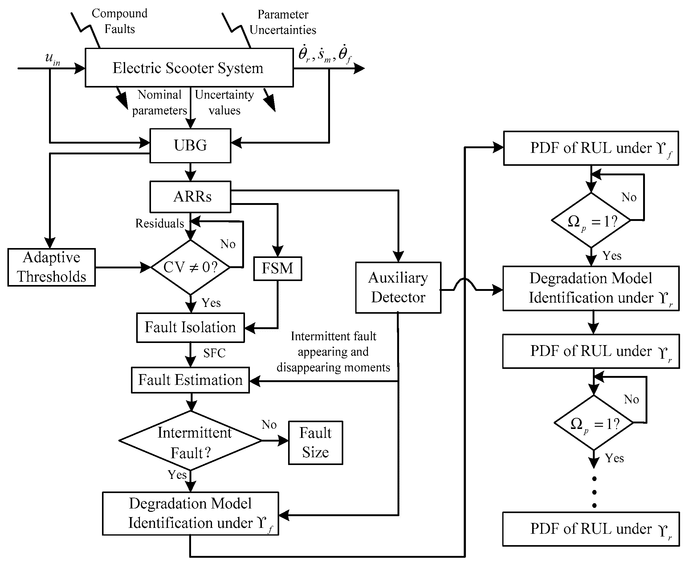
3. Fault Estimation and Sequential Prognosis

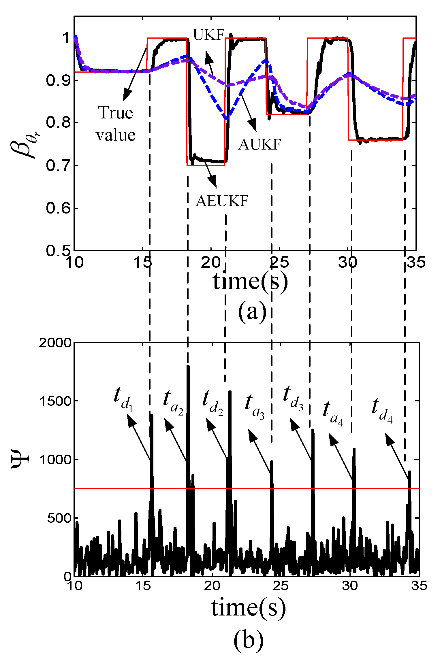
3.1. Fault Estimation Scheme

Once the SFC is obtained after FDI, the next step is to determine the fault severity and its type. In this paper, the un-scented Kalman filtering (UKF) is adopted for the joint estimation of state and fault (parametric and nonparametric) in the nonlinear scooter system. The UKF is a stochastic nonlinear filtering method which inherits the well-known features of Kalman filter. Unlike the extended Kalman filter (EKF), which needs the linearization of nonlinear models, UKF uses the unscented transform (UT) to select the finite set of sigma points, and then propagates these sigma points directly through the nonlinear models to approximate the state mean and covariance estimates. More details of UKF can be found in [28].
To implement the UKF for the joint estimation of state and fault, the scooter state x k = [ θ r , k θ ˙ r , k s m , k s ˙ m , k θ f , k θ ˙ f , k ] T ( k is the discrete time index) needs to be augmented as x a u g , k = [ x k ϕ ] T , where ϕ denotes the vector which includes all fault parameters in the SFC. Based on x a u g , k , the nonlinear discrete stochastic model of the electric scooter can be given as follows
{ x a u g , k = f ( x a u g , k 1 , w k ) y k = h ( x a u g , k , v k )
where f ( ) is the nonlinear state transition function, h ( ) is the measurement function, y k = [ θ ˙ r , k s ˙ m , k θ ˙ f , k ] T is the vector of measured velocities, w k is the process noise with covariance Q k , v k is the measurement noise with covariance R k .
The generic UKF cannot be directly applied to the nonlinear electric scooter system due to the following two reasons: (1) the generic UKF is not geared towards tracking sudden parameter changes of intermittent fault parameter. This is because that the diagonal terms of the posteriori state error covariance, denoted by P k | k , automatically decrease to show more confidence in the estimation as the filter attempts to converge to the true parameter value. When a sudden parameter change occurs, the filter does follow the change, but its convergence is slow due to the small P k | k . This leads to a problem that if the next sudden change happens before the filter converges to the true fault value, the fault estimator cannot finish its task; (2) the sensors used for measuring the angular velocities and longitudinal speed are susceptible to the stochastic vibration when the scooter runs, and the modeling errors due to modelling simplifications and assumptions are inevitable. Therefore, the process noise and measurement noise covariances are time-varying and unknown.
To remedy the aforementioned two problems, the AEUKF, which can simultaneously expedite the tracking of sudden changes and estimate the unknown process noise and measurement noise covariances, is proposed. To achieve AEUKF, two major modifications are made on the generic UKF. The first modification lies in the enhancement of P k | k to restore the filter ability to track the sudden change. This enhancement can be implemented as follows
{ Ψ Ψ 0 P k | k = τ P k | k Ψ < Ψ 0 P k | k = P k | k
with
Ψ = i = 1 3 η i | d 2 r i , n d t 2 |
where Ψ is the auxiliary detector, Ψ 0 is the threshold of the auxiliary detector, τ is the enhancement factor, η i = 1 if ith ARR is inconsistent, and η i = 0 otherwise.
In (6), the auxiliary detector Ψ is used to detect the sudden changes. The choice of Ψ stems from the fact that the sudden changes can be captured by the sum of absolute values of second derivative of inconsistent ARRs due to the use of integral to obtain position from velocity in (2)–(4). Once a sudden change is detected by auxiliary detector, the covariance P k | k is enhanced to compensate for the generic UKF latency.
The second modification aims to adaptively estimate the process noise covariance Q k and measurement noise covariance R k using the output velocity residual sequence of the scooter model. This method is known as covariance matching which can be represented as follows [29]
{ Q k = K k C k K k T R k = i = 0 2 n W c i ( y k | k 1 i y k + C k ) ( y k | k 1 i y k + C k ) T
with
C k = i = k L + 1 k e i e i T L
where e i is the velocity residual, C k is the covariance of the velocity residual, n is the dimension of x a u g , k , y k | k 1 i is the ith predicted (a priori) velocity in sigma points, K k is the Kalman gain, W c i is the i th covariance weight, and L is window size for covariance matching. In the nonlinear discrete stochastic model, all fault parameters in the set of fault candidates are augmented into the system original state. Thus, the model can replicate the system behavior after fault occurrence because the fault parameters embedded into the model can be estimated by using the augmented model. Therefore, the estimation of the process noise covariance and measurement noise covariance is not affected by the fault occurrence.

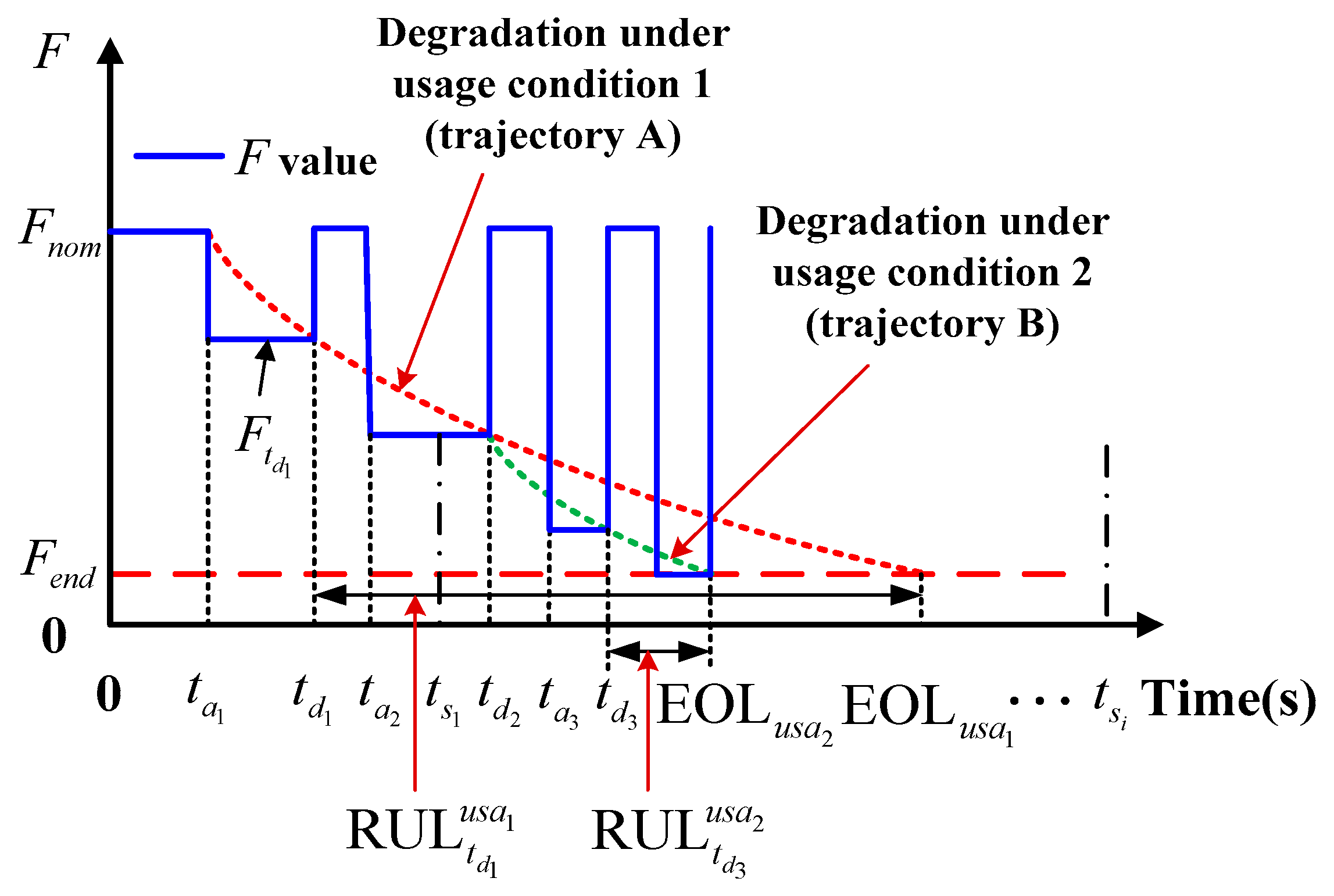
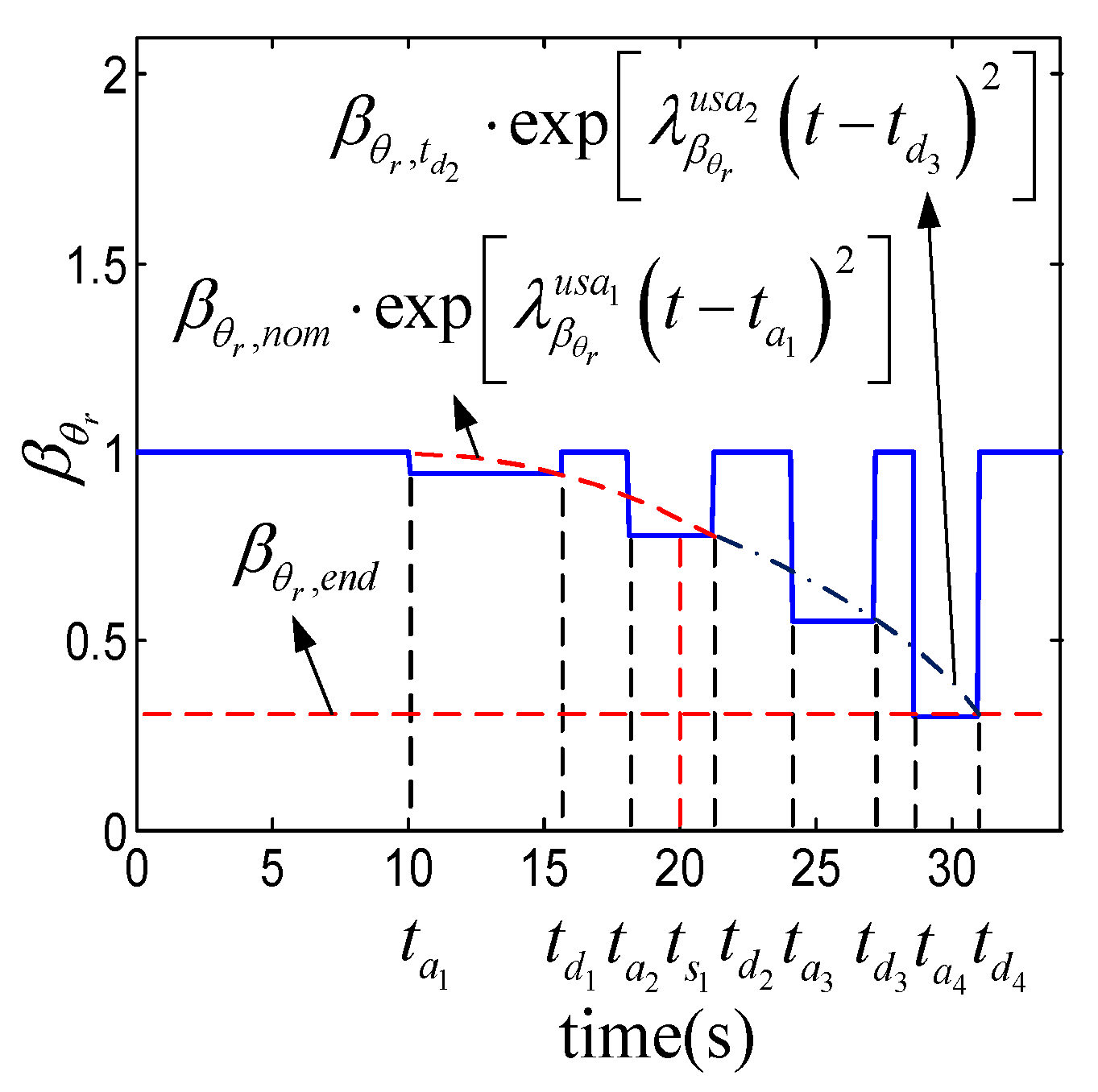
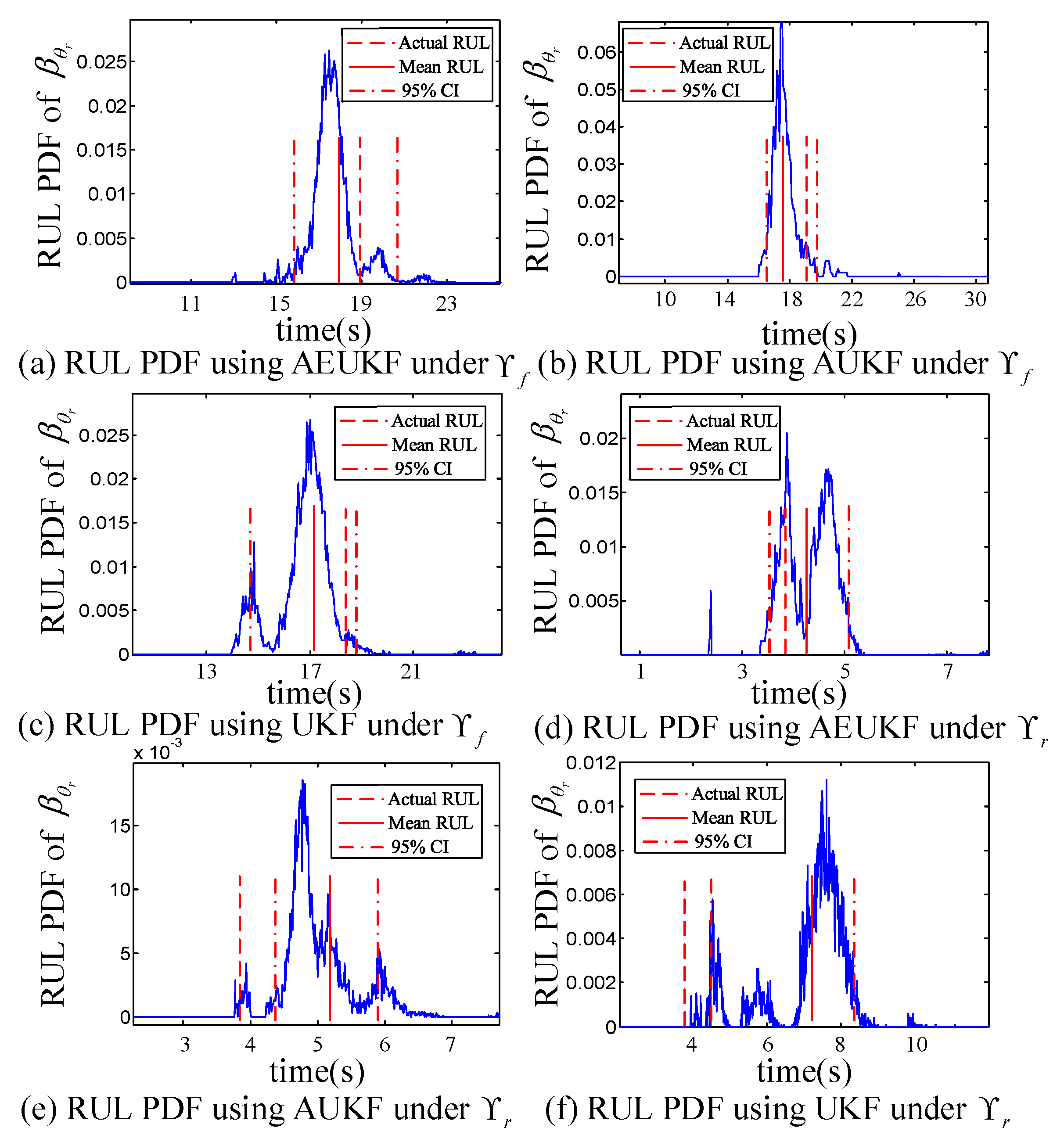
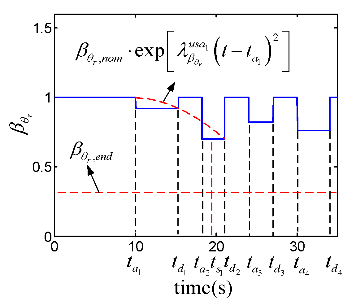
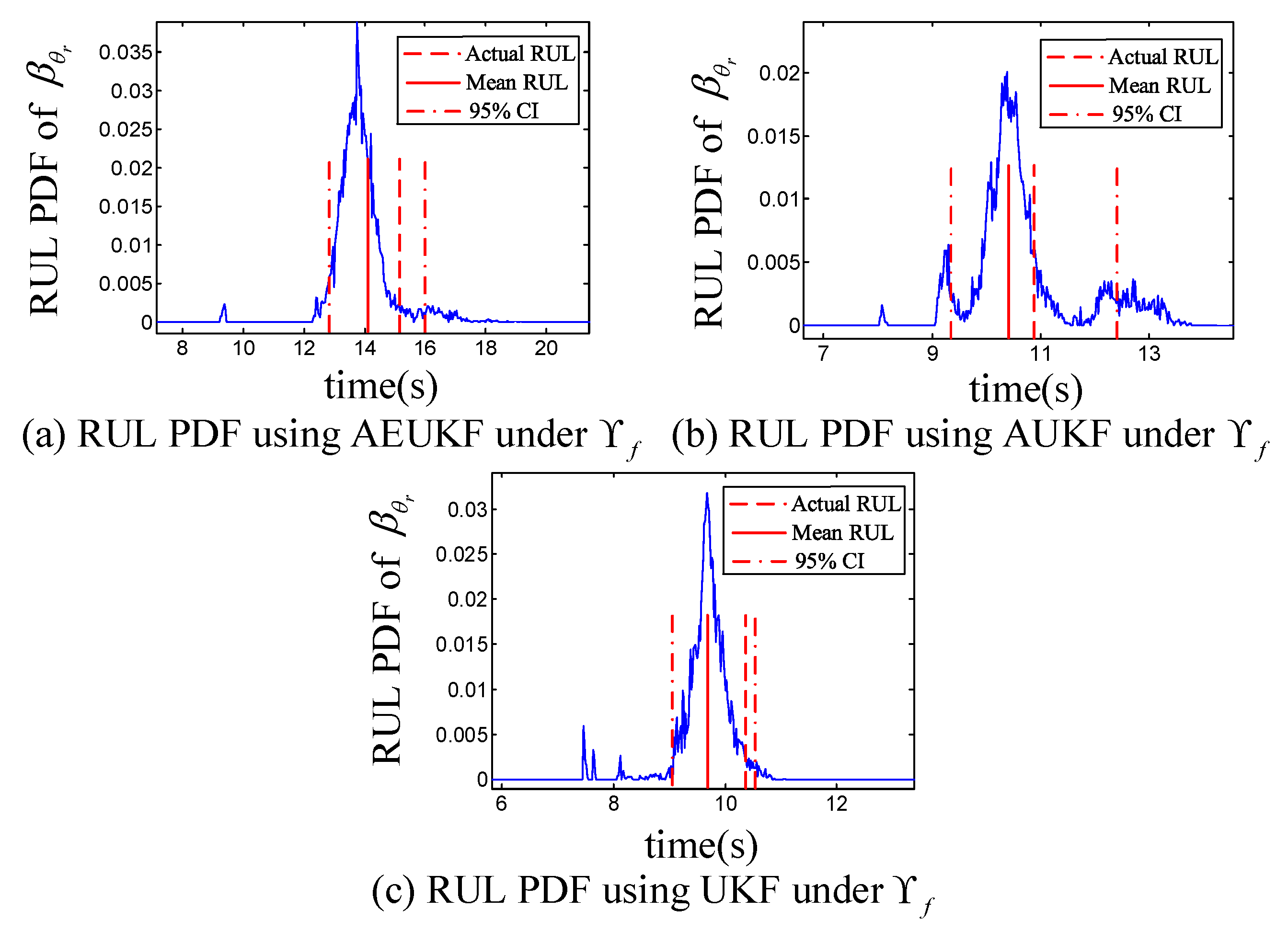
3.2. Sequential Prognosis

After fault estimation, the fault type and its magnitude can be obtained. Given the estimated fault trajectory, one may treat this fault as abrupt fault if the estimated value almost keeps constant. On the other hand, the fault can be considered as intermittent fault if the estimated fault trajectory exhibits obviously sudden increasing (or decreasing) trend. To predict the possible future trajectories of the intermittent fault for RUL prediction, a certain degradation model is required to describe its degradation trend. Note that the degradation is usually dependent on the operating conditions. For instance, the degradation rate of bearing in electric fan is different at different speed levels. Motivated by this observation, the following usage dependent degradation model is developed
{ F = F ¯ e [ d F u s a j ( t t ¯ ) ] , d F u s a j = λ F u s a j ( t t ¯ ) , t ¯ = t a 1 , F ¯ = F n o m t ¯ = t d k s i , F ¯ = F t d k s i if Υ f if Υ r
where F n o m is the parameter nominal value, t a 1 is the first fault appearing time, t d k s i is the smallest t d k satisfying t d k > t s i where t d k , k = 1 , 2 , , is the fault disappearing time, t s i , i = 1 , 2 , , is the usage change time and F t d k s i is the fault value at t d k s i , d F u s a j is the degradation rate, λ F u s a j is the usage dependent degradation coefficient, Υ f denotes t a 1 < t < t d k s i , Υ r represents t d k s i < t < t d k s i + 1 , j = 1 in Υ f , and j = i + 1 in Υ r .
The proposed usage dependent degradation profile is illustrated in Figure 3. In F axis, F denotes the parameter value or efficiency factor value in both normal and faulty conditions by which the evolution of the value over time can be demonstrated. In the figure, the usage is changed at t s 1 from condition 1 to condition 2 (indicates a severer operating condition). As a result, the degradation coefficient increases which causes the fault progression to follow another trajectory (i.e., from trajectory A to trajectory B) as shown in Figure 3. Therefore, the EOL time EOL u s a 2 (its related RUL is RUL t d 3 u s a 2 ) at which the failure threshold F e n d is reached under usage condition 2 is shorter than the EOL time EOL u s a 1 (its related RUL is RUL t d 1 u s a 1 ) under usage condition 1. Note that in Figure 3, the fault values at the disappearing moments constitute the degradation curve and the fault value at each appearing intervals is considered to be constant. In this way, the degradation process of intermittent fault occurring in random discontinuous intervals can be established which in turn allows the development of RUL prediction algorithm under changing usage conditions.
The AEUKF-based fault estimator constantly and recursively updates the unknown fault values after FDI, but the prognoser is only reactivated at time t ¯ d k s i (denotes the second smallest t d k satisfying t d k > t s i since two detected instants and two estimated fault values are required to identify the degradation model parameters under Υ r ) if some prescribed events are detected. Note that if the estimated intermittent fault evolution is found to be non-monotonic due to the usage condition change, the prognoser will not be reactivated even if the usage change is observed. Moreover, other factors (e.g., the relation between the fault value at t ¯ d k s i and F e n d , and the minimum number of estimates required to identify the degradation model under Υ r ) also determine the reactivation of prognoser. Thus, under Υ r , the following logic is defined to describe the reactivation of the prognoser at t ¯ d k s i
Ω p = { 1 , 0 , if E V 1 = 1 E V 2 = 1 E V 3 = 1 E V 4 = 1 otherwise
with
E V 1 = { 1 , if sign ( F t ¯ d k s i F t d k s i ) = sign ( F t d 1 F n o m ) 0 , otherwise
E V 2 = { 1 , if F t ¯ d k s i does not exceed F e n d 0 , otherwise
E V 3 = { 1 , if N t d k 2 for t ( t s i , t s i + 1 ) 0 , otherwise
E V 4 = { 1 , if usage change occurs at t s i 0 , otherwise
where represents logic AND, Ω p { 0 , 1 } is a binary variable denoting the reactivation state of prognoser, where Ω p = 1 denotes that prognoser is reactivated, and Ω p = 0 otherwise.
The degradation process is generally irreversible and degradation cannot decrease. In this paper, what increases or decreases is the value of fault parameter in different components. For example, the resistance value in the circuit may increase or decrease abnormally due to fault but the degradation of the resistance increases. In (9), E V 1 = 1 indicates that the degradation characteristic (i.e., monotonic increase or monotonic decrease of value of fault parameter) after the usage change occurs is consistent with the one before the usage change occurs. Otherwise, the degradation is treated as a non-monotonic process and the prognoser will not be reactivated. As a result, the RUL under the new usage condition cannot be predicted. The event E V 2 = 1 describes that the fault value at t ¯ d k s i (denoted by F t ¯ d k s i ) does not hit F e n d . The event E V 3 = 1 suggests that at least two fault estimates are required to identify the degradation model parameters under Υ r , where N t d k denotes the number of disappearing instants within time interval ( t s i , t s i + 1 ) . The event E V 4 = 1 indicates that a change of usage condition is observed. It is obvious that the prognoser can be reactivated provided that the four events are detected.
Under Υ f , the prognoser is enabled at t d 1 that is captured by the auxiliary detector. There are two unknown parameters ( t a 1 and λ F u s a 1 ) in (8). Since the fault detection module can detect t a 1 , the unknown parameter λ F u s a 1 can be solved as
λ F u s a 1 = ln ( F ^ t d 1 / F n o m ) / ( t d 1 t a 1 ) 2
where F ^ t d 1 is the estimated fault value at t d 1 .
Thus, the EOL u s a 1 can be computed from (8) and (10) as
EOL u s a 1 = ln ( F e n d / F n o m ) / λ F u s a 1 + t a 1
Based on (11), the RUL under Υ f can be calculated as
RUL t d 1 u s a 1 = EOL u s a 1 t d 1
Under Υ r , if the prognoser is reactivated (i.e., Ω p = 1 ) at t ¯ d k s i , three unknown parameters ( λ F u s a j , t d k s i and F t d k s i ) exist in (8). Here t d k s i can be detected by the auxiliary detector, and F t d k s i can be obtained by the fault estimator. Therefore, the unknown parameter λ F u s a j can be computed as
λ F u s a j = ln ( F ^ t ¯ d k s i / F ^ t d k s i ) / ( t ¯ d k s i t d k s i ) 2
where F ^ t ¯ d k s i and F ^ t d k s i are the fault estimates at t ¯ d k s i and t d k s i , respectively.
Thus, the EOL u s a j can be derived as
EOL u s a j = ln ( F e n d / F ^ t d k s i ) / λ F u s a j + t d k s i
The RUL under Υ r can be formulated as
RUL t ¯ d k s i u s a j = EOL u s a j t ¯ d k s i
In order to recovery the predicted RUL distribution and thus estimate the RUL uncertainty, the Monte Carlo simulation (MCS) approach is utilized to draw M samples to generate all possible future trajectories as follows [16]:
F i N ( F ^ , P F ^ ) , i = 1 , 2 , , M
where F ^ = F ^ t d 1 under Υ f and F ^ = [ F ^ t d k s i ,   F ^ t ¯ d k s i ] under Υ f , and P F ^ represents the diagonal terms of the state error covariance related to the estimated fault values.
According to (10)–(16), M possible RUL predictions are
RUL i = { EOL u s a 1 i t d 1 if Υ f EOL u s a j i t ¯ d k s i if Υ r , i = 1 , 2 , , M
where EOL u s a 1 i is the EOL of ith sample under Υ f , and EOL u s a j i is the EOL of ith sample under Υ r .
From (17), the predicted mean RUL can be computed as
RUL m e a n = 1 M i = 1 M RUL i
The complete flow chart of the proposed method is presented in Figure 4. In the FDI step, the adaptive threshold is adopted to detect the fault under parameter uncertainties and then SFC is obtained by comparing the nonzero CV with the FSM. The SFC includes the possible faults with unknown types. During fault estimation, the AEUKF-based estimator identifies the fault values and distinguishes the fault types with the aid of auxiliary detector. If the fault type is intermittent, degradation model identification is carried out using the information from the fault estimation and auxiliary detector. Given the predefined failure threshold, the probability distribution function (PDF) of RUL under Υ f can be predicted. In order to reactivate the prognoser, four associated events are judged. If the prognoser is reactivated, the fault estimation results and the information from the auxiliary detector are again used for the identification of degradation model under Υ r , where the degradation coefficient under the new usage condition can be calculated. With the newly calculated degradation coefficient and failure threshold, the PDF of RUL under Υ r can be computed statistically by the MCS method.

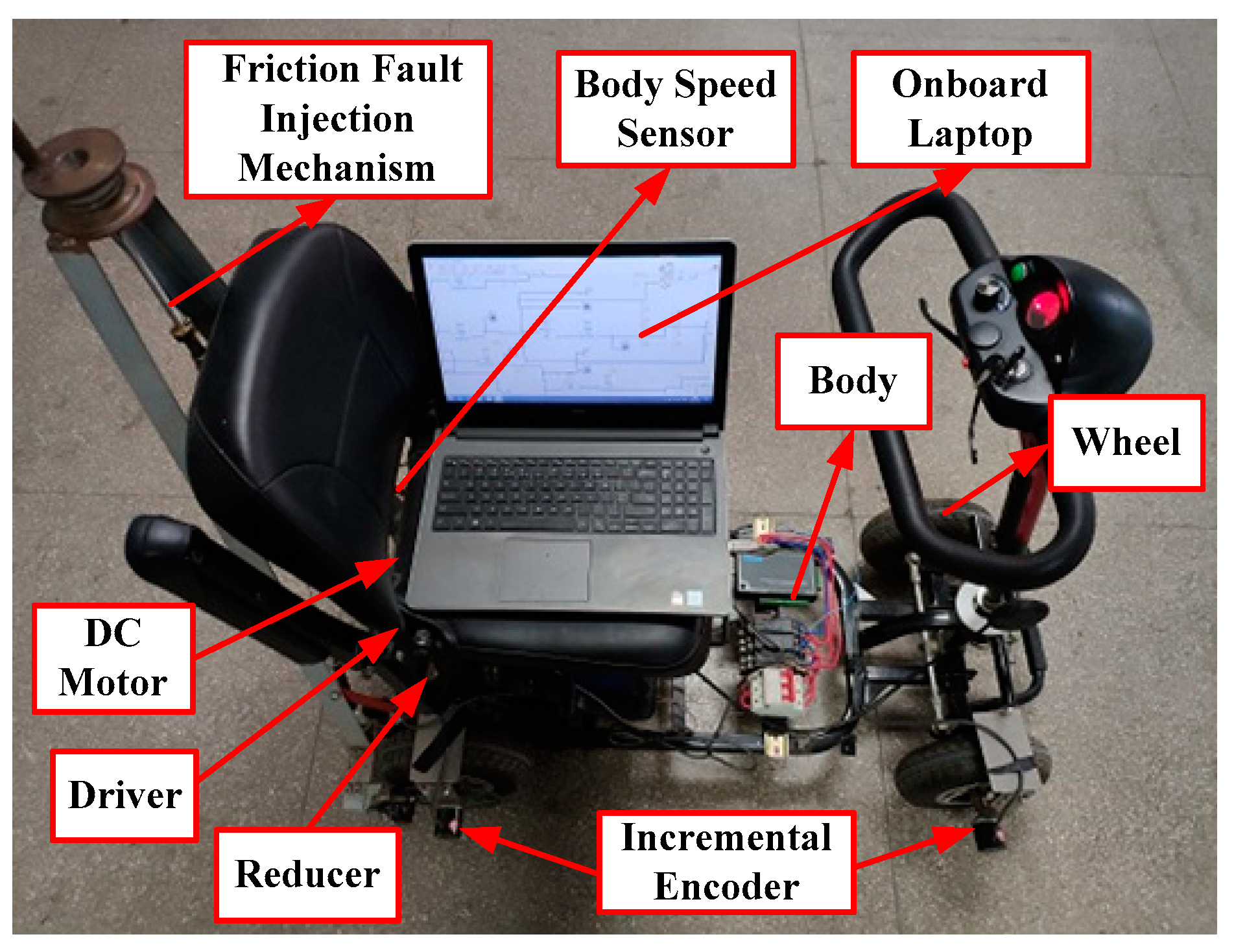
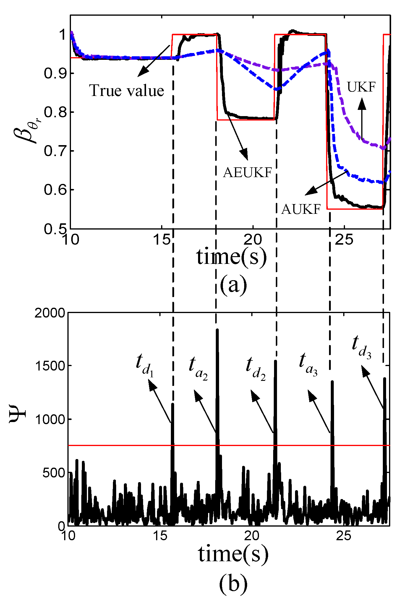
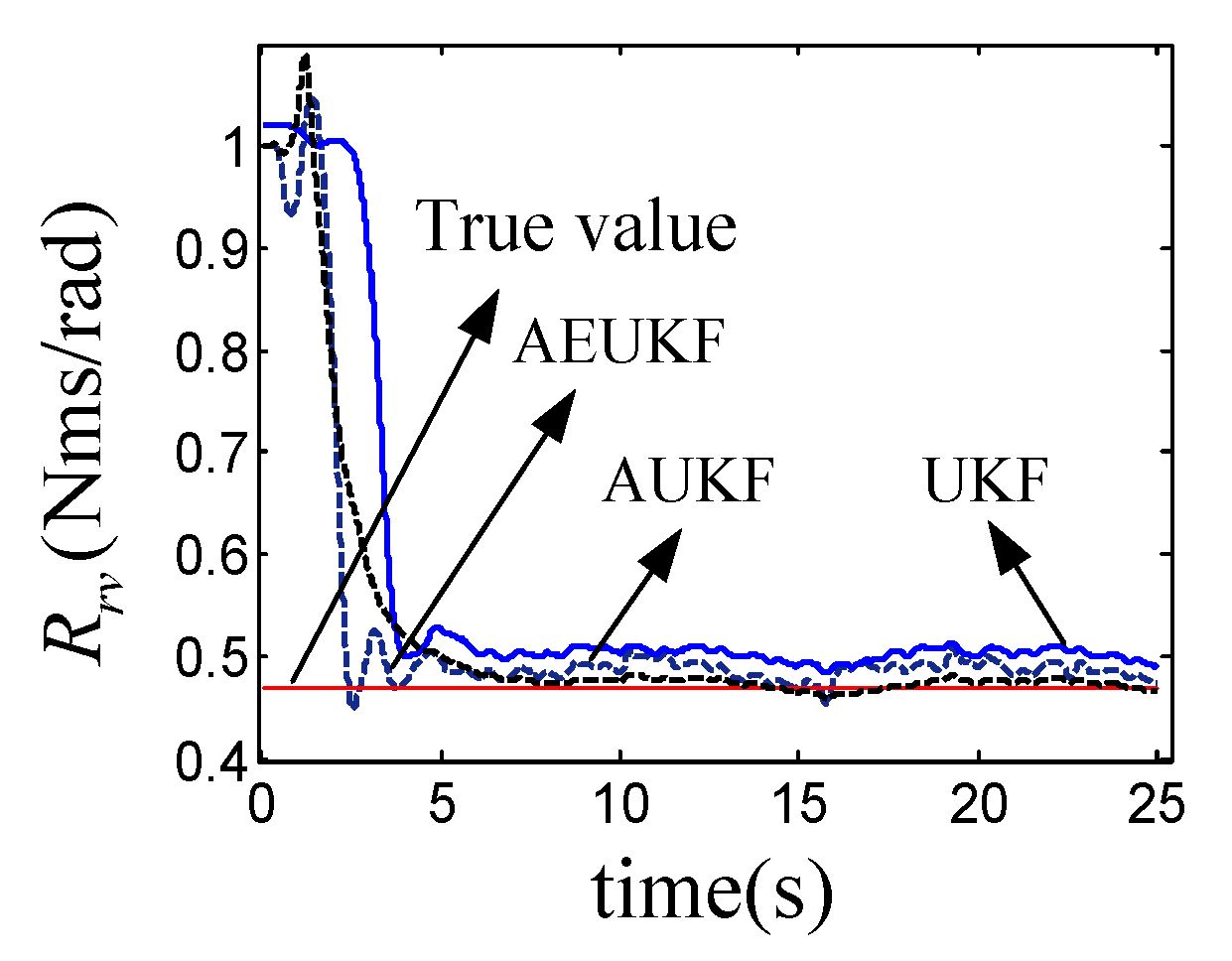
4. Experiment Results

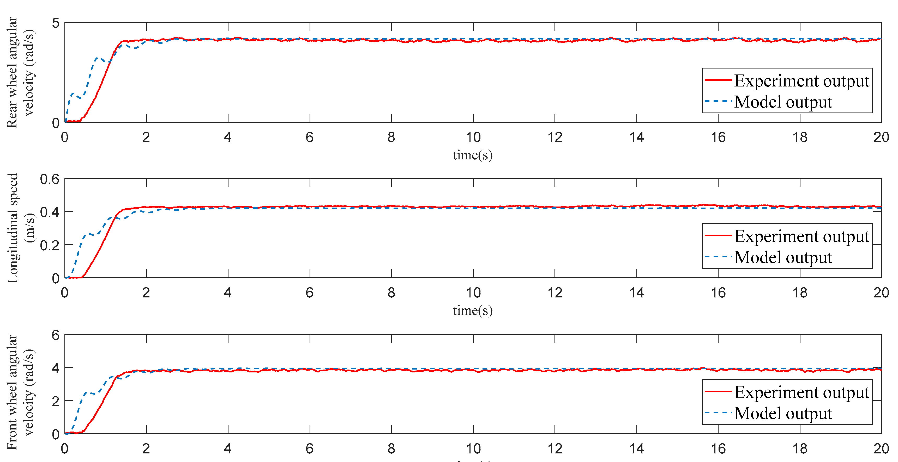
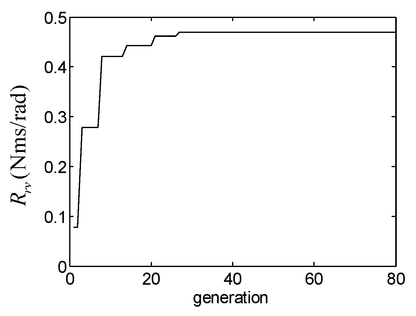
4.1. Parameter Identification and Model Validation

In order to evaluate the performance of the proposed fault diagnosis and prognosis method, the nominal parameter values and the respective multiplicative uncertainty values should be properly identified so that the developed model can capture the dynamic behavior of the monitored electric scooter system. Some parameter values are taken from the manufacture specifications, so that no uncertainties are defined for these parameters. It is more meaningful to consider uncertainties for other parameters (e.g., friction) because they are more prone to be affected by the usage conditions. Other parameter values are identified by the genetic algorithm (GA) [30]. In this paper, the two-point crossover operator and the single-point mutation operator are used in GA, where the values of the crossover probability and the mutation probability are 0.8 and 0.07, respectively. The fitness function for parameter identification is defined as
F f i t n e s s = 1 / ( j = 1 l ( | r 1 n j | + | r 2 n j | + | r 3 n j | ) + ε )
where l is the number of the collected data and ε is a small positive constant to avoid division by zero during the optimization process.
Ten sets of input–output data using the same command input signal 1 V are obtained from the actual electric scooter system. Each set is used for parameter identification based on GA with the fitness function in (19). For each parameter, the mean calculated from the ten sets of identified parameters is treated as the nominal value, and the maximum deviation from the mean value divided by the mean value is considered as the multiplicative uncertainty value [7].
The identification results are given in Table 3. In order to validate the developed model using the identified parameters, the same input signal 1 V is applied to the model and the real system. The comparison between the model and the system outputs is given in Figure 5. From the figure, it is observed that the model outputs show agreement with the actual outputs of the electric scooter system.

4.2. Experimental Results

For the experimental setup in Figure 1, three sensors and motor are powered by two 12 V batteries. The sensors and associated hardware measures the scooter velocities and then send them to the onboard laptop via USB data acquisition card (Advantech USB 4711A) and LabVIEW software. The onboard laptop also provides power to the USB data acquisition card and sends command input signal to the motor driver. FDI is implemented by the standard LabVIEW module, while fault estimation and RUL prediction are conducted by utilizing the MATLAB script node in LabVIEW environment where the co-simulation between MATLAB and LabVIEW can be implemented online.
Two experiments under compound faults are conducted. The first one concerns an abrupt friction fault in R r v on the rear wheel and a monotonic intermittent sensor fault in β θ r . A special mechanical arrangement in Figure 1 is fabricated to introduce the friction fault in R r v . The mechanism consists of rotary disc, steel wire, and rubber sheet. The rotary disc can be manually rotated to drive the steel wire connected with the rubber sheet. The steel wire can control the distance between rubber sheet and the rear wheel. Under normal condition, the rubber sheet and the rear wheel are totally separated. When the rubber sheet is engaged with the rear wheel, the rear wheel friction is increased and the fault severity is determined by the rotation angle of the rotary disc. When the abrupt friction fault is injected, the rotation angle of the rotary disc under this fault condition is marked. For reference purpose, the abrupt fault value of R r v is needed and thus, the GA based fault identification (only suitable for the case of abrupt fault) is adopted, where only R r v is the unknown parameter and other parameter values are taken from Table 3. Figure 6 shows the identification result where the identified R r v = 0.469 Nms/rad.
The intermittent fault profile is given in Figure 7. The designed fault appearing and disappearing moments are t a 1 = 10 s, t d 1 = 15.56 s, t a 2 = 18 s, t d 2 = 21.16 s, t a 3 = 24 s, t d 3 = 27.08 s, t a 4 = 28.5 s, t d 4 = 30.94 s, and the fault values at the appearing interval are 0.94, 0.78, 0.55 and 0.3. The failure threshold β θ r , e n d = 0.3. The input representing the usage condition is changed from 1 V to 1.2 V at t s 1 = 19.8 s. The degradation coefficient λ β θ r u s a 1 = 0.002 under Υ f and λ β θ r u s a 2 = 0.01 under Υ r . The designed RUL is 18.98 s under Υ f and 3.86 s under Υ r .
The residual responses are shown in Figure 8. The nonlinear discrete model in (5) is obtained by discretizing the continuous model in (2)–(4) using Euler’s backward difference method. To guarantee the discrete model accuracy, the sampling time should be short enough. On the other hand, the sampling time must be long enough to assure the real time computation of the developed method. Thus, a tradeoff is made where the sampling time is chosen as 0.02 s. From Figure 8, a CV = [1 1 0] is detected after 10 s and the SFC is { β θ r , K 1 , β θ r & R r v , β θ r & K 1 , β θ r & R r v & K 1 , R r v & K 1 } . After that, the fault estimation is activated where AEUKF, AUKF and UKF are employed for comparison purpose [29]. The initial parameters for all filters are selected as P 0 = diag(0.01, 0.01, 0.01, 0.01, 0.01, 0.01, 0.5, 0.3, 20), Q 0 = diag(0.01, 0.01, 0.01, 0.01, 0.01, 0.01, 0.01, 0.01, 0.01), and R 0 = diag(0.2, 0.2, 0.2). Figure 9a shows the estimate of β θ r and Figure 9b illustrates the response of Ψ where the dashed line is the threshold of the auxiliary detector Ψ 0 = 760 . The Ψ is calculated by the derivative function in LabVIEW. Since the choice of τ in (6) is critical for the AEUKF, a set of experiments are conducted to choose τ properly. It is found that the performance of sudden change tracking improves with the increase of τ . However, when τ increases beyond 5, poor tracking performances (i.e., large estimate fluctuations during sudden change instants and deteriorations in tracking error) occur. As a result, τ is set to be 5. It is observed from Figure 9a that UKF and AUKF do attempt to follow the step changes, but the convergence is too slow to track the true value before next sudden change occur. By contrast, the AEUKF can ensure the prompt tracking of the sudden changes by enhancing the posteriori state error covariance timely with the aid of the auxiliary detector Ψ . The estimated values of R r v (shown in Figure 10) using AEUKF, AUKF and UKF, are 0.463 Nms/rad, 0.478 Nms/rad and 0.487 Nms/rad, respectively, which are close to the actual fault value (i.e., 0.469 Nms/rad). The estimated values of K 1 (shown in Figure 11) using AEUKF, AUKF and UKF, respectively, are 10.09 Nm/rad, 10.14 Nms/rad and 9. 85 Nm/rad, which are close to the nominal one (i.e., 10.02 Nm/rad). As the result, the K 1 is excluded from the SFC. To show the average performance of fault estimation algorithms, more experiments (i.e., 6 sets of experiments) are conducted where the corresponding results are summarized in Table 4. In the table, L i , i = 1 , 2 , 3 , represents the time period between t a i and t d i . It was found that AEUKF and AUKF are superior to UKF, owing to the employment of the covariance matching technique.
Since the identified fault type of β θ r is intermittent based on Figure 9a, the RUL is statistically predicted via the MCS method with M = 80. Figure 12a–c, respectively, show the predicted RUL PDF based on the AEUKF, AUKF and UKF under Υ f . The predicted mean RUL is 17.87 s for AEUKF, 17.83 s for AUKF, and 17.19 s for UKF. The actual RUL under Υ f stays within 95% confidence interval (CI) for all filters. The AUKF and UKF are acceptable since no step change occurs before t d 1 (i.e., AUKF and UKF do not exhibit estimation latency before t d 1 ). In order to quantitatively compare the prognosis performance of different methods, two metrics, i.e., relative accuracy (RA) for prediction accuracy and relative standard deviation (RSD) for prediction spread, are adopted [14]. The performance results under usage 1 are given in Table 5 where the metrics are expressed in percentages. From the table, it is observed that all methods yield good RA (i.e., over 90%) and RSD (i.e., under 10%). The performance of AUKF is almost the same as that of AEUKF. The slight decrease in performance of UKF is due to the difficulty of setting noise covariances.
After t s 1 , the usage condition is changed which causes the degradation to follow another trajectory as shown in Figure 7. The prognoser is reactivated at t d 3 since Ω p = 1 . From Figure 9a, the AUKF and UKF cannot rapidly track the step changes which could adversely affect the subsequent degradation coefficient calculation and RUL prediction. Figure 12d–f, respectively, illustrate the predicted RUL PDF using the AEUKF, AUKF and UKF under Υ r . The predicted mean RUL is 4.21 s for AEUKF, which is close to the actual value (i.e., 3.86 s). The actual RUL falls inside the 95% CI. However, as expected, improper RUL predictions occur for AUKF and UKF, where the actual RUL falls outside the 95% CI. This is due to the overestimations of fault values which stems from the lack of ability to promptly track the sudden changes. As a result, the RUL predictions by the AUKF and UKF are not acceptable. The prognosis performances under usage 2 is shown in Table 5 where the mark “ × ” in the entry indicates an unacceptable prediction metric.
In the second experiment, an abrupt fault in R r v and a non-monotonic intermittent fault in β θ r (whose profile is given in Figure 13) are introduced. The designed fault appearing and disappearing moments are t a 1 = 10 s, t d 1 = 15.3 s, t a 2 = 19.2 s, t d 2 = 21 s, t a 3 = 24 s, t d 3 = 27 s, t a 4 = 30 s, t d 4 = 34 s, and the designed fault values at the appearing interval are 0.92, 0.7, 0.82 and 0.76. The failure threshold β θ r , e n d = 0.3. The input representing the usage condition is changed from 1 V to 1.3 V at t s 1 = 19.7 s. The degradation coefficient λ β θ r u s a 1 = −0.003 and the designed RUL is 14.8 s under Υ f . The RUL under Υ r is not available since the degradation is non-monotonic after t s 1 . The residual responses are presented in Figure 14 where a CV = [1 1 0] is observed after 10 s and the resulting SFC is { β θ r , K 1 , β θ r & R r v , β θ r & K 1 , β θ r & R r v & K 1 , R r v & K 1 } . The fault estimation is then enabled where AEUKF, AUKF and UKF are adopted.
The estimation results are given in Figure 15 where the AEUKF can ensure the timely tracking of sudden changes with the help of the auxiliary detector, but UKF and AUKF cannot work well. The estimated values of R r v using AEUKF, AUKF and UKF, are 0.461 Nms/rad, 0.447 Nms/rad and 0.445 Nms/rad, respectively. The estimated values of K 1 using AEUKF, AUKF and UKF, respectively, are 9.94 Nm/rad, 9.91 Nms/rad and 10. 15 Nm/rad, which are close to the nominal one. Thus, the K 1 is not a fault candidate and R r v is an abrupt fault. Table 6 shows the average estimation results of 6 sets of experiments. In the table, L i , i = 1 , 2 , 3 , 4 , represents the time period between t a i and t d i . From the Table 6, it is observed that the AEUKF performs best among all methods.
The RUL prediction is carried out for β θ r with M = 80. Figure 16a–c, respectively, give the predicted RUL PDF based on the AEUKF, AUKF and UKF under Υ f . The predicted mean RUL is 14.07 s for AEUKF, 13.84 s for AUKF, and 13.42 s for UKF. For all methods, the actual RUL remains within 95% CI. The prognosis performances of different methods are shown in Table 5. It was observed that AUKF and AEUKF achieve similar performance since no sudden change occurs before t d 1 , while UKF performance decreases slightly. After t s 1 , the usage condition is changed where the degradation characteristic is non-monotonic as shown in Figure 13. Thus, E V 1 = 1 is not satisfied and the prognoser will not be reactivated at t d 3 . As a result, the RUL of β θ r under the new usage condition cannot be predicted.

5. Conclusions

In this paper, a UBG based FDI of compound faults and an AEUKF-based fault estimation and sequential prognosis are developed for an electric scooter with parameter uncertainties. The compound faults of unknown types are considered, and the auxiliary detector aided AEUKF is proposed to distinguish the fault types, track the sudden changes of intermittent fault, and estimate the unknown noise covariances. For the sequential prognosis of intermittent fault in the presence of non-monotonic degradation, a set of reactivation events are defined, and the prognoser is only reactivated if all these events are satisfied. The efficiency of the proposed methodology is verified by experiment results.

Author Contributions

Conceptualization, M.Y.; methodology, H.L.; software, D.L.; validation, C.X.; formal analysis, H.W.; writing—original draft preparation, M.Y. All authors have read and agreed to the published version of the manuscript.

Funding

This work was supported in part by the National Natural Science Foundation of China under Grant 61673154.

Conflicts of Interest

The authors declare no conflict of interest.

References

  1. Gao, Z.; Cecati, C.; Ding, S.X. A survey of fault diagnosis and fault-tolerant techniques-part I: Fault diagnosis with model-based and signal-based approach. IEEE Trans. Ind. Electron. 2015, 62, 3757–3767. [Google Scholar] [CrossRef] [Green Version]
  2. Liu, X.; Gao, Z.; Chen, M.Z.Q. Takagi-Sugeno fuzzy model based fault estimation and signal compensation with application to wind turbines. IEEE Trans. Ind. Electron. 2017, 64, 5678–5689. [Google Scholar] [CrossRef]
  3. Blesa, J.; Jiménez, P.; Rotondo, D.; Nejjari, F.; Puig, V. An interval NLPV parity equations approach for fault detection and isolation of a wind farm. IEEE Trans. Ind. Electron. 2015, 62, 3794–3805. [Google Scholar] [CrossRef] [Green Version]
  4. Verma, N.K.; Sevakula, R.K.; Dixit, S.; Salour, A. Intelligent condition based monitoring using acoustic signals for air compressors. IEEE Trans. Reliab. 2016, 65, 291–309. [Google Scholar] [CrossRef]
  5. Li, R.; He, D. Rotational machine health monitoring and fault detection using EMD-based acoustic emission feature quantification. IEEE Trans. Instrum. Meas. 2012, 61, 990–1001. [Google Scholar] [CrossRef]
  6. Benmoussa, S.; Bouamama, B.O.; Merzouki, R. Bond graph approach for plant fault detection and isolation: Application to intelligent autonomous vehicle. IEEE Trans. Autom. Sci. Eng. 2014, 11, 585–593. [Google Scholar] [CrossRef]
  7. Djeziri, M.A.; Merzouki, R.; Bouamama, B.O.; Dauphin-Tanguy, G. Robust fault diagnosis by using bond graph approach. IEEE/ASME Trans. Mechatron. 2007, 12, 599–611. [Google Scholar] [CrossRef]
  8. Zhang, X.; Polycarpou, M.M.; Parisini, T. A robust detection and isolation scheme for abrupt and incipient faults in nonlinear systems. IEEE Trans. Automat. Control. 2002, 47, 576–593. [Google Scholar] [CrossRef]
  9. Zhang, X.; Parisini, T.; Polycarpou, M.M. Adaptive fault-tolerant control of nonlinear uncertain systems: An information-based diagnostic approach. IEEE Trans. Automat. Control. 2004, 49, 1259–1274. [Google Scholar] [CrossRef]
  10. Kolar, D.; Lisjak, D.; Pająk, M.; Pavković, D. Fault diagnosis of rotary machines using deep convolutional neural network with wide three axis vibration signal input. Sensors 2020, 20, 4017. [Google Scholar] [CrossRef]
  11. Pająk, M.; Muślewski, Ł.; Landowski, B.; Grządziela, A. Fuzzy identification of the reliability state of the mine detecting ship propulsion system. Pol. Marit. Res. 2019, 26, 55–64. [Google Scholar] [CrossRef] [Green Version]
  12. Nguyen, V.; Seshadrinath, J.; Wang, D.; Nadarajan, S.; Vaiyapuri, V. Model-based diagnosis and RUL estimation of induction machines under interturn fault. IEEE Trans. Ind. Appl. 2017, 53, 2690–2701. [Google Scholar] [CrossRef]
  13. Yu, M.; Wang, D.; Luo, M. An integrated approach to prognosis of hybrid systems with unknown mode changes. IEEE Trans. Ind. Electron. 2015, 62, 503–515. [Google Scholar] [CrossRef]
  14. Pająk, M. Fuzzy identification of a threat of the inability state occurrence. J. Intell. Fuzzy Syst. 2018, 35, 3593–3604. [Google Scholar] [CrossRef]
  15. Pająk, M. Fuzzy model of the operational potential consumption process of a complex technical system. Facta Univ. Ser. Mech. Eng. 2020, 18, 453–472. [Google Scholar]
  16. Daigle, M.; Bregon, A.; Roychoudhury, I. Distributed prognostics based on structural model decomposition. IEEE Trans. Reliab. 2016, 63, 495–510. [Google Scholar] [CrossRef] [Green Version]
  17. Hu, X.; Jiang, J.; Cao, D.; Egardt, B. Battery health prognosis for electric vehicles using sample entropy and sparse Bayesian predictive modeling. IEEE Trans. Ind. Electron. 2016, 63, 2645–2655. [Google Scholar] [CrossRef]
  18. Climente-Alarcon, V.; Antonino-Daviu, J.A.; Strangas, E.G.; Riera-Guasp, M. Rotor-bar breakage mechanism and prognosis in an induction motor. IEEE Trans. Ind. Electron. 2015, 62, 1814–1825. [Google Scholar] [CrossRef] [Green Version]
  19. Gucik-Derigny, D.; Outbib, R.; Ouladsine, M. A comparative study of unknown-input observers for prognosis applied to an electromechanical system. IEEE Trans. Reliab. 2016, 65, 704–717. [Google Scholar] [CrossRef]
  20. Ompusunggu, A.P.; Papy, J.; Vandenplas, S. Kalman-filtering-based prognostics for automatic transmission clutches. IEEE/ASME Trans. Mechatron. 2016, 21, 419–430. [Google Scholar] [CrossRef]
  21. Lei, Y.; Xie, H.; Yuan, Y.; Chang, Q. Fault location for the intermittent connection problems on CAN networks. IEEE Trans. Ind. Electron. 2015, 62, 7203–7213. [Google Scholar] [CrossRef]
  22. Obeid, N.H.; Battiston, A.; Boileau, T.; Nahid-Mobarakeh, B. Early intermittent interturn fault detection and localization for a permanent magnet synchronous motor of electrical vehicles using wavelet transform. IEEE Trans. Transp. Electrif. 2017, 3, 694–702. [Google Scholar] [CrossRef]
  23. Yan, R.; He, X.; Wang, Z.; Zhou, D. Detection, isolation and diagnosability analysis of intermittent faults in stochastic systems. Int. J. Control 2018, 91, 480–494. [Google Scholar] [CrossRef]
  24. Hu, S.; Wang, L.; Mao, J.; Gao, C.; Zhang, B.; Yang, S. Synchronous online diagnosis of multiple cable intermittent faults based on chaotic spread spectrum sequence. IEEE Trans. Ind. Electron. 2019, 66, 3217–3226. [Google Scholar] [CrossRef]
  25. Auzanneau, F. Detection and characterization of microsecond intermittent faults in wired networks. IEEE Trans. Instrum. Meas. 2018, 67, 2256–2258. [Google Scholar] [CrossRef]
  26. Syed, W.; Perinpanayagam, S.; Samie, M.; Jennions, I. A novel intermittent fault detection algorithm and health monitoring for electronic interconnections. IEEE Trans. Compon. Packag. Manuf. Technol. 2016, 6, 400–406. [Google Scholar] [CrossRef] [Green Version]
  27. Borutzky, W. Bond graph model-based system mode identification and mode-dependent fault thresholds for hybrid systems. Math. Comput. Model. Dyn. Syst. 2014, 20, 584–615. [Google Scholar] [CrossRef]
  28. Partovibakhsh, M.; Liu, G. An adaptive unscented Kalman filtering approach for online estimation of model parameters and state-of-charge of lithium-ion batteries for autonomous mobile robots. IEEE Trans. Control Syst. Technol. 2015, 23, 357–363. [Google Scholar] [CrossRef]
  29. Meng, J.; Luo, G.; Gao, F. Lithium polymer battery state-of-charge estimation based on adaptive unscented Kalman filter and support vector machine. IEEE Trans. Power Electron. 2016, 31, 2226–2238. [Google Scholar] [CrossRef]
  30. Arogeti, S.; Wang, D.; Low, C.B.; Yu, M. Fault detection isolation and estimation in a vehicle steering system. IEEE Trans. Ind. Electron. 2012, 59, 4810–4820. [Google Scholar] [CrossRef]
Figure 1. Electric scooter system.
Actuators 09 00128 g001
Figure 2. Uncertain bond graph (UBG) of the electric scooter.
Actuators 09 00128 g002
Figure 3. Usage dependent degradation process of intermittent fault.
Actuators 09 00128 g003
Figure 4. Flow chart of the proposed method.
Actuators 09 00128 g004
Figure 5. Model outputs versus experiment outputs.
Actuators 09 00128 g005
Figure 6. Identification of R r v .
Actuators 09 00128 g006
Figure 7. Fault profile in β θ r .
Actuators 09 00128 g007
Figure 8. Residual responses of experiment.
Actuators 09 00128 g008
Figure 9. Estimation results: (a) Estimate of β θ r ; (b) Response of Ψ .
Actuators 09 00128 g009
Figure 10. Estimate of R r v .
Actuators 09 00128 g010
Figure 11. Estimate of K 1 .
Actuators 09 00128 g011
Figure 12. β θ r RUL prediction results.
Actuators 09 00128 g012
Figure 13. Fault profile in β θ r .
Actuators 09 00128 g013
Figure 14. Residual responses of experiment.
Actuators 09 00128 g014
Figure 15. Estimation results: (a) Estimate of β θ r ; (b) Response of Ψ .
Actuators 09 00128 g015
Figure 16. β θ r RUL prediction results.
Actuators 09 00128 g016
Table 1. Nomenclatures.
VariableNomenclatureVariableNomenclature
u i n Input signal R m v Motor viscous friction
R 1 Electrical resistance of the motor R m c Motor Coulomb friction
N 1 Voltage-to-current constant R r v Rear wheel viscous friction
N 2 Current-to-torque ratio R r c Rear wheel Coulomb friction
N 3 Reduction ratio R f v Front wheel viscous friction
N 4 Wheel radius R f c Front wheel Coulomb friction
J m Motor inertia s m Longitudinal displacement
R m Motor mechanical friction θ f Angular position of front wheel
R f Front wheel friction θ r Angular position of rear wheel
R r Rear wheel friction a Adaptive threshold
K 1 ; K 2 Transmission axis rigidity r Analytical redundancy relation
s ˙ m Longitudinal speed J f Front wheel inertial
θ ˙ f Angular velocity of front wheel δ Multiplicative uncertainty
θ ˙ r Angular velocity of rear wheel β Efficiency factor
J r Rear wheel inertial w Additional effort source
Table 2. Fault signature matrix (FSM) of the electric scooter.
A R R 1 A R R 2 A R R 3 D b
R r v 1 0 01
β θ r 1 1 01
K 1 1 1 01
N 4 1111
β s m 1 1 11
β θ f 0 1 11
β f v 0 0 11
Table 3. Nominal parameter and multiplicative uncertainty values.
Nominal ValueUncertainty Value Nominal ValueUncertainty Value
N 1 3 A/V/ J r 4.87 × 10 3   kgm 2 2.84%
N 2 0.0666 Nm/A/ J f 6.97   × 10 3   kgm 2 2.76%
N 3 1/18/ R r v 3.545   × 10 2 Nms/rad5.12%
N 4 0.115 m/ R r c 5.955   × 10 2 Nm1.89%
R 1 1.03 Ω 2.61% R f v 1.02   × 10 3 Nms/rad2.79%
R m v 1.725 × 10 3 Nms/rad2.98% R f c 1.857   × 10 3 Nm2.91%
R m c 5.635 × 10 2 Nm5.86% K 1 10.02 Nm/rad2.29%
J m 5.03 × 10 4 kgm 2 8.12% K 2 10.07 Nm/rad1.13%
m 20.7 kg2.06%
Table 4. Comparison of fault estimation performance.
β θ r R r v   ( Nms / rad ) K 1   ( Nm / rad )
L 1 L 2 L 3
Actual value0.940.780.550.46910.02
MeanAEUKF0.950.790.560.46310.05
AUKF0.960.850.620.47710.09
UKF0.960.910.700.4879.88
St.devAEUKF0.00110.00120.00110.00120.06
AUKF0.00160.00160.00170.00150.11
UKF0.00220.00210.00220.00230.14
Table 5. Comparison of remaining useful life (RUL) prediction performance.
RARSD
Experiment1Usage1UKF90.579.57
AUKF93.949.06
AEUKF94.159.32
Usage2UKF × ×
AUKF × ×
AEUKF90.7111.59
Experiment2Usage1UKF90.688.31
AUKF93.518.25
AEUKF95.078.28
Table 6. Comparison of fault estimation performance.
β θ r R r v   ( Nms / rad ) K 1   ( Nm / rad )
L 1 L 2 L 3 L 4
Actual value0.920.700.820.760.46910.02
AEUKF0.920.720.830.760.4629.98
MeanAUKF0.920.810.830.850.4489.93
UKF0.930.890.840.860.44310.12
AEUKF0.00110.00130.00110.00120.00130.06
St.devAUKF0.00160.00170.00150.00170.00190.12
UKF0.00220.00220.00230.00210.00230.13
Publisher’s Note: MDPI stays neutral with regard to jurisdictional claims in published maps and institutional affiliations.

