Observer-Based Tracking Control for Polysolenoid Linear Motor with Unknown Disturbance Load

Abstract

Linear motors have been playing a crucial role in mechanical motion systems due to its ability to provide a straight motion directly without mediate mechanical actuators. This paper investigates tracking control problems of Polysolenoid Linear Motor, which is a particular type of permanent magnet linear motor in a tubular structure. In order to deal with unmeasurable velocity, our method proposes a novel observer guaranteed asymptotic convergence of the observer errors. Then, based on observed velocity, our method proposes controllers for position-velocity and current tracking control concerning an unknown disturbance load problem by using Lyapunov direct method. The proposed controllers ensure that the position-velocity tracking error converges to arbitrarily small values by adjusting control parameters. Finally, the validity and effectiveness of our approach are shown in illustrative examples.

1. Introduction

Linear Motor motion systems have been widely applied to fruitful applications in order to provide directed straight motions in which, unnecessary mechanical transmissions are excluded that results in better performance and lost-cost requirement of motion systems [1]. Recently, there has been a great deal of effort devoted to control design for linear motors in various topics including motion control theory [2,3], the planar motion of a nanopositioning platform [4], traction systems for subway [5] and jetting dispenser [6]. As a particular case, polysolenoid linear motor (PLM) belongs to the group of permanent magnet linear motor in tubular structure as shown in Figure 1. The motor has two phases corresponding to two separated windings working differently in 90° of electrical angle. The usage of PLM brings some beneficial properties such as the durable structure, low cost, and reliable operations according to an electromagnetic phenomenon with principles as shown in [7,8]. More recently, various research topics focus on control design for PLM such as model predictive control [9,10] and flatness based control structure [11].

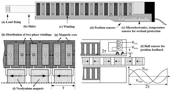
Figure 1. Structure of polysolenoid linear motor provided by [7,27].

Without the needs of any gearbox for motion transformation, the movement of linear motor systems become sensitive due to external impacts such as frictional force, changed load and non-sine of flux. The disturbance force impacts in both the longitudinal and in the transversal direction, which results in harmful effects to system performance. Over the past few years, there have been several kinds of research spending amounts of effort to deal with position tracking problems of linear motor systems in the presence of external disturbances. A neural network learning adaptive robust controller was designed by [12] to achieve both tracking performance and disturbance rejection. Besides, compensation approaches were proposed in researches [13,14,15], by which the frictional force and position-dependent disturbance are compensated to guarantee the stability of the overall system. The researches in [16,17,18] present effective sliding mode control methods for tracking control of the linear motor.

In the progress of disturbances rejection methods, sensorless control problems of a linear permanent-magnet motor have been received a lot of attention from fruitful researches including linear tubular motors [19,20], end-effects [21,22], position sensorless control [23,24]. Generally, for a class of permanent-magnet synchronous motor, almost all researches use back electromotive force (EMF), which are observed via currents and voltages, to estimate the velocity of the linear motor. As a matter of fact, at low and zero speed, the back electromotive force (EMF) voltage magnitude is very small, or zero, and this makes all the techniques based on the back EMF unsuccessful [25,26]. Besides, the main problems of the approach are disturbance impacts in currents and voltages. Furthermore, the variation in inductance parameters due to some main characteristics of the linear motor, such as end effect, may result in considerable estimation error. On the other hand, almost PLMs are packed with at least one position sensor, and Figure 2 describes the typical control scheme of PLM. However, when the sensors are affected by measurement noise, velocity is not obtained accurately by taking derivatives respect to specific interval time.

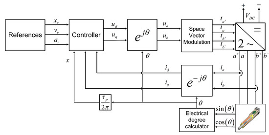
Figure 2. Typical control scheme of polysolenoid linear motor.

Inspired by the above observations, this paper addresses tracking problems of Polysolenoid Linear Motor under unknown load disturbance effect. In the light of novel observer-based control approach, our research covers a realistic problem arsing when the velocity of PLM can not be measured by using directly position sensor can not be calculated by using data from position sensor. To summarize, our contributions can be highlighted as

• A novel velocity observer has been proposed such that the observer errors exponentially converge by utilizing the available position sensors attached in PLM. To be specific, based on Lyapunov theorem, the exponential convergence of observer errors has been proofed in a rigorous way. Furthermore, conditions for selecting parameters of the observer are provided as well as delay rate of the observer errors.
• From the observer, a position-velocity and current controllers are designed by Lyapunov direct method. Accordingly, the position or velocity tracking error converge to small arbitrary values by adjusting control parameters.

This paper is organized as follows. Section 2 establishes main problems and a mathematical model of the PLM in $d-q$ axis. In Section 3, a novel velocity observer is proposed, and asymptotic convergence of observer errors are proofed. Section 4 mainly describes position-velocity and current controller design. Section 5 illustrates the simulation results for verification of the proposed method. Finally, conclusions are summarized in Section 6.

2. Problem Statement

As mentioned above, the PLM has two separated windings $a,b$ and is supplied by two AC voltage sources as follow

$$\begin{array}{c}\hfill u_a\left(t\right)=Ucos\left(\omega t\right),u_b=Usin\left(\omega t\right).\end{array}$$

(1)

Further, angular electrical position of PLMs inducing in the windings has the relationship with the primary position, and electrical angular frequency can be expressed as

$$\begin{array}{c}\hfill \theta \left(t\right)=\frac{n_p\pi }{\tau }x\left(t\right),\omega \left(t\right)=\frac{n_p\pi }{\tau }v\left(t\right).\end{array}$$

(2)

By neglecting the friction terms in mechanical equation, let us take into account dynamic model of Polysolenoid Linear Motor (PLM) in $d-q$ frame given in as follow

$$\begin{array}{cc}\hfill & \hfill \frac{dx}{dt}=v\left(t\right),\end{array}$$

(3)

$$\begin{array}{cc}\hfill & \hfill \frac{dv}{dt}=\frac{2\pi {\psi }_p}{m{\tau }_p}{i}_q\left(t\right)-\frac{1}{m}{f}_{\ell }\left(t\right)-\frac{1}{m}{f}_m\left(t\right),\end{array}$$

(4)

$$\begin{array}{cc}\hfill & \hfill \frac{d{i}_d}{dt}=-\frac{R_s}{L}{i}_d\left(t\right)+\left(\frac{2\pi }{{\tau }_p}v\left(t\right)\right)i_q\left(t\right)+\frac{1}{L}{u}_d\left(t\right),\end{array}$$

(5)

$$\begin{array}{cc}\hfill & \hfill \frac{d{i}_q}{dt}=-\frac{R_s}{L}{i}_q\left(t\right)-\left(\frac{2\pi }{{\tau }_p}v\left(t\right)\right)i_d\left(t\right)-\left(\frac{2\pi }{{\tau }_p}v\left(t\right)\right)\frac{{\psi }_p}{L}+\frac{1}{L}{u}_q\left(t\right),\end{array}$$

(6)

where ${\tau }_p=\frac{\tau }{n_p},$$i_d\left(t\right),i_q\left(t\right)$ are the direct and quadrature stator current; $v\left(t\right),x\left(t\right)$ denote linear velocity and position of rotor; $R_s,L$ represent for phase resistance, and stator inductances; ${\psi }_p,m$ stand for the flux of the permanent magnet and mass of slider (rotor), respectively. The inputs of system are the direct and quadrature voltage which are denoted as $u_d\left(t\right),u_q\left(t\right)$. Additionally, $f_{\ell }\left(t\right)$ is disturbance load and $f_m\left(t\right)$ represents for a combination of detent force (including cogging and ending force [28]) and the force generated by inductance fluctuation [29].

In what follows, let $x_r\left(t\right),v_r\left(t\right)$, respectively, are stator’s desired position and velocity of the PLM. This note aims to design a position-velocity controller, by which the actual position and velocity can track these references with small errors. It should be noted that the PLM in industrial applications often does not include a velocity sensor. Unlike rotor rotation motors where velocity sensors can be easily employed by attaching in rotor shape, the velocity sensor equipment for PLM increases enormous additional cost, and it is difficulties in installing and restricted by environmental factors like temperature, humidity and vibration as well. Therefore, the paper develops a novel velocity observer that utilizes the available position sensors in PLM to estimate velocity. Furthermore, the proposed controllers also guarantee robust performance in the presence of unknown disturbance load variations. In views of control performance, the rotor angular position must track a reference trajectory $x_r\left(t\right)$. Additionally, to avoid reluctance effects and force ripple, $i_d\left(t\right)$ should track a constant direct current reference $i_{dr}\left(t\right)=0$. The following sections present the observer and controller synthesis for position tracking of PLM.

3. Observer Design

To cover more realistic situations in industrial applications, we provide a velocity observer to deal with the velocity sensorless problem. For simplicity’s sake, let $f\left(t\right)=\frac{1}{m}{f}_{\ell }\left(t\right)+\frac{1}{m}{f}_m\left(t\right)$. In this paper, we deal with the continuous disturbance $f\left(t\right)$ such that

$$\begin{array}{c}\hfill \left|f\left(t\right)\right|\le \overline{F},\left|\dot{f}\left(t\right)\right|\le \overline{\delta F},\end{array}$$

(7)

in which $\overline{F}$ and $\overline{\delta F}$ are given positive constants. Let us provide the following observer as

$$\begin{array}{c}\hfill \begin{array}{cc}\hfill \dot{\widehat{x}}\left(t\right)& =\widehat{v}\left(t\right)+h_1\left(x\left(t\right)-\widehat{x}\left(t\right)\right),\hfill \\ \hfill \dot{\widehat{v}}\left(t\right)& =\frac{2\pi {\psi }_p}{m{\tau }_p}{i}_q\left(t\right)+h_2\left(x\left(t\right)-\widehat{x}\left(t\right)\right)+K\mathrm{sign}\left(x\left(t\right)-\widehat{x}\left(t\right)\right),\hfill \end{array}\end{array}$$

(8)

where $h_1,h_2,K$ are real positive constants. By denoting $\tilde{x}\left(t\right)=x\left(t\right)-\widehat{x}\left(t\right)$ and $\tilde{v}\left(t\right)=v\left(t\right)-\widehat{v}\left(t\right)$, the dynamics of observer errors are given by the combination of (3), (4) and (8):

$$\begin{array}{c}\hfill \begin{array}{cc}\hfill \dot{\tilde{x}}\left(t\right)& =-h_1\tilde{x}\left(t\right)+\tilde{v}\left(t\right),\hfill \\ \hfill \dot{\tilde{v}}\left(t\right)& =-h_2\tilde{x}\left(t\right)-K\mathrm{sign}\left(\tilde{x}\left(t\right)\right)-f\left(t\right).\hfill \end{array}\end{array}$$

(9)

Theorem 1.

For a given $\alpha >0$, let K, $h_1$, $h_2$ are positive constants satisfying

$$\begin{array}{cc}\hfill & \left[\begin{array}{cc}{h}_1{h}_2& 0\\ 0& h_1\end{array}\right]\ge 2\alpha \left[\begin{array}{cc}{h}_2+\frac{1}{2}{h}_1^2& \frac{1}{2}{h}_1\\ \frac{1}{2}{h}_1& 1\end{array}\right],\hfill \end{array}$$

(10)

$$\begin{array}{cc}\hfill & \frac{K{h}_1}{2}-\frac{h_1\overline{F}}{2}-\overline{\delta F}\ge 2\alpha (K+\overline{F}).\hfill \end{array}$$

(11)

Then, the system (9) is exponentially stable. Furthermore, there exist ${\beta }_1,{\beta }_2>0$ such that

$$\begin{array}{c}\hfill |\tilde{x}\left(t\right)|<{\beta }_1{e}^{-\alpha t},|-h_1\tilde{x}\left(t\right)+\tilde{v}\left(t\right)|<{\beta }_2{e}^{-\alpha t}.\end{array}$$

(12)

Proof Theorem 1.

Letting ${\eta }_1\left(t\right)=\tilde{x}\left(t\right)$, ${\eta }_2\left(t\right)=-h_1\tilde{x}\left(t\right)+\tilde{v}\left(t\right)$ and $\eta \left(t\right)={[{\eta }_1\left(t\right),{\eta }_2\left(t\right)]}^T$, then (9) can be rewritten as

$$\begin{array}{c}\hfill \begin{array}{cc}\hfill {\dot{\eta }}_1\left(t\right)& ={\eta }_2\left(t\right),\hfill \\ \hfill {\dot{\eta }}_2\left(t\right)& =-h_1\dot{\tilde{x}}\left(t\right)+\dot{\tilde{v}}\left(t\right)\hfill \\ \hfill & =-h_1{\eta }_2\left(t\right)-h_2{\eta }_1\left(t\right)-K\mathrm{sign}\left({\eta }_1\left(t\right)\right)-f\left(t\right).\hfill \end{array}\end{array}$$

(13)

Consider the following function

$$\begin{array}{c}\hfill V_o(t,\eta \left(t\right))=\frac{1}{2}{\eta }_2{\left(t\right)}^2+\left(\frac{h_2}{2}+\frac{h_1^2}{4}\right){\eta }_1{\left(t\right)}^2+K\left|{\eta }_1\left(t\right)\right|+f\left(t\right){\eta }_1\left(t\right)+\frac{h_1}{2}{\eta }_1\left(t\right){\eta }_2\left(t\right).\end{array}$$

(14)

From the fact that $K>\overline{F}$, we have $K|{\eta }_1\left(t\right)|>|f\left(t\right){\eta }_1\left(t\right)|$. Then, $V_o(t,\eta \left(t\right))$ is a positive real function, and especially it has $V_o(t,0)=0$, $V_o(t,\eta \left(t\right))>0\forall \eta \left(t\right)\ne 0$, and $V_o(t,\eta \left(t\right))\to \infty$ as $\left|\right|\eta \left(t\right)\left|\right|\to \infty$. Hence, the time derivative of the Lyapunov function (14) along the solution of (13) is given by

$$\begin{array}{cc}\hfill {\dot{V}}_o(t,\eta \left(t\right))& ={\eta }_2\left(t\right){\dot{\eta }}_2\left(t\right)+\left(h_2+\frac{h_1^2}{2}\right){\eta }_1\left(t\right){\eta }_2\left(t\right)+K{\eta }_2\left(t\right)\mathrm{sign}\left({\eta }_1\left(t\right)\right)+f\left(t\right){\eta }_2\left(t\right)+\dot{f}\left(t\right){\eta }_1\left(t\right)\hfill \\ \hfill & +\frac{h_1}{2}{\eta }_2{\left(t\right)}^2+\frac{h_1}{2}{\eta }_1\left(t\right){\dot{\eta }}_2\left(t\right)\hfill \\ \hfill & =-\frac{h_1}{2}{\eta }_2{\left(t\right)}^2+\dot{f}\left(t\right){\eta }_1\left(t\right)+\frac{h_1}{2}{\eta }_1\left(t\right)\left(-h_2{\eta }_1\left(t\right)-K\mathrm{sign}\left({\eta }_1\left(t\right)\right)-f\left(t\right)\right)\hfill \\ \hfill & =-\frac{h_1}{2}{\eta }_2{\left(t\right)}^2-\frac{h_1{h}_2}{2}{\eta }_1{\left(t\right)}^2+{\eta }_1\left(t\right)\left(-\frac{K{h}_1}{2}\mathrm{sign}\left({\eta }_1\left(t\right)\right)-\frac{h_1}{2}f\left(t\right)+\dot{f}\left(t\right)\right).\hfill \end{array}$$

(15)

Recalling K in Theorem 1 and (7), it is worth remarking that

$$\begin{array}{c}\hfill \frac{K{h}_1}{2}>\frac{h_1\overline{F}}{2}+\overline{\delta F}>\left|\frac{h_1}{2}f\left(t\right)-\dot{f}\left(t\right)\right|.\end{array}$$

(16)

Using the fact that ${\eta }_1\left(t\right)\mathrm{sign}\left({\eta }_1\left(t\right)\right)=\left|{\eta }_1\left(t\right)\right|$, and multiplying both sides of (1) by $|{\eta }_1\left(t\right)|$ leads to

$$\begin{array}{c}\hfill \frac{K{h}_1}{2}{\eta }_1\left(t\right)\mathrm{sign}\left({\eta }_1\left(t\right)\right)\ge \left(\frac{h_1\overline{F}}{2}+\overline{\delta F}\right)\left|{\eta }_1\left(t\right)\right|\ge \left|{\eta }_1\left(t\right)\left(\frac{h_1}{2}f\left(t\right)-\dot{f}\left(t\right)\right)\right|.\end{array}$$

As a result,

$$\begin{array}{cc}\hfill {\eta }_1\left(t\right)\left(\frac{K{h}_1}{2}\mathrm{sign}\left({\eta }_1\left(t\right)\right)-\frac{h_1}{2}f\left(t\right)+\dot{f}\left(t\right)\right)& \ge \frac{K{h}_1}{2}\left|{\eta }_1\left(t\right)\right|-\left|{\eta }_1\left(t\right)\left(\frac{h_1}{2}f\left(t\right)-\dot{f}\left(t\right)\right)\right|\hfill \\ \hfill & \ge \frac{K{h}_1}{2}|{\eta }_1\left(t\right)|-\left(\frac{h_1\overline{F}}{2}+\overline{\delta F}\right)\left|{\eta }_1\left(t\right)\right|.\hfill \end{array}$$

Therefore, from (15), it follows that

$$\begin{array}{c}\hfill {\dot{V}}_o(t,\eta \left(t\right))\le -\frac{h_1}{2}{\eta }_2{\left(t\right)}^2-\frac{h_1{h}_2}{2}{\eta }_1{\left(t\right)}^2-\left(\frac{K{h}_1}{2}-\frac{h_1\overline{F}}{2}-\overline{\delta F}\right)\left|{\eta }_1\left(t\right)\right|.\end{array}$$

(17)

On the other hand, it can be derived from (14) that

$$\begin{array}{c}\hfill V_o(t,\eta \left(t\right))\le \frac{1}{2}{\eta }^T\left(t\right)\left[\begin{array}{cc}{h}_2+\frac{1}{2}{h}_1^2& \frac{1}{2}{h}_1\\ \frac{1}{2}{h}_1& 1\end{array}\right]\eta \left(t\right)+(K+\overline{F})\left|{\eta }_1\left(t\right)\right|.\end{array}$$

(18)

As the result, from condition (10) and (11), it derived that ${\dot{V}}_o(t,\eta \left(t\right))\le -2\alpha V_o(t,\eta \left(t\right))$. By using comparison lemma in ([30], Lemma 3.4), we obtain

$$\begin{array}{c}\hfill V_o(t,\eta \left(t\right))\le V_o(0,\eta \left(0\right))e^{-2\alpha t}.\end{array}$$

(19)

Accordingly, ${\eta }_1\left(t\right)$ and ${\eta }_2\left(t\right)$ exponentially converge. Further, exist ${\beta }_1,{\beta }_2>0$ such that ${\eta }_1^2\left(t\right)<{\beta }_1^2{V}_o(t,\eta \left(t\right))$, ${\eta }_2^2\left(t\right)<{\beta }_2^2{V}_o(t,\eta \left(t\right))$. Intuitively, the proof of Theorem 1 is completed. □

Remark 1.

In the case the load disturbance $F_{\ell }\left(t\right)$ is excluded ($F_{\ell }\left(t\right)\equiv 0$), the switching term in (8) can be removed. In this case, the observer (8) can be reduced as high-gain observer founded in [31]. Hence, our proposed observer can be considered as an extension of high-gain observer to handle the influence of disturbance.

4. Controller Design

In the view of control strategy, the dynamic model (3)–(6) can be separated into two subsystems named as position-velocity and current subsystem. It worth noting that the current subsystem possesses much faster dynamics than that of the position-velocity subsystem. By taking cascade control into account, our method establishes an inner and outer control loop corresponding to the current and position-velocity subsystem.

4.1. Position-Velocity Subsystem

As a convenience, we denote desired velocity and acceleration corresponding to $v_r\left(t\right)={\dot{x}}_r\left(t\right)$, $a_r\left(t\right)={\dot{v}}_r\left(t\right)$. Additionally, the following notations are applied

$$\begin{array}{c}\hfill \sigma =\frac{2\pi \psi }{m{\tau }_p},e_x\left(t\right)=x\left(t\right)-x_r\left(t\right),e_v\left(t\right)=v\left(t\right)-v_r\left(t\right),{\widehat{e}}_v\left(t\right)=\widehat{v}\left(t\right)-v_r\left(t\right),\end{array}$$

(20)

to rewrite position-velocity subsystem in (3) and (4) as

$$\begin{array}{c}\hfill \begin{array}{cc}\hfill {\dot{e}}_x\left(t\right)& =e_v\left(t\right),\hfill \\ \hfill {\dot{e}}_v\left(t\right)& =\sigma i_q^{*}-a_r\left(t\right)-f\left(t\right),\hfill \end{array}\end{array}$$

(21)

where the notation “$i_q^{*}$” indicates the desired quadrature current which is entrusted to current control loop. In this paper, we assume $i_q\left(t\right)$ simultaneously track $i_q^{*}$. According, $i_q^{*}$ replaces $i_q\left(t\right)$ in (21). The following theorem provides a controller for

Theorem 2.

Let us consider

$$\begin{array}{c}\hfill i_q^{*}=\frac{1}{\sigma }\left(a_r\left(t\right)-K_x{e}_x\left(t\right)-K_v{\widehat{e}}_v\left(t\right)\right),\end{array}$$

(22)

where $K_x,K_v$ are real positive constants. Then, the system (21) is stable, and $e_x\left(t\right),e_v\left(t\right)$ converge to a arbitrary small values by choosing large enough control parameters $K_x,K_v$.

Proof Theorem 2.

Recalling notations in (20), it is obtained that ${\widehat{e}}_v\left(t\right)=e_v\left(t\right)-\tilde{v}\left(t\right)$. Then, (21) can be rearranged as

$$\begin{array}{c}\hfill \begin{array}{cc}\hfill {\dot{e}}_x\left(t\right)& =e_v\left(t\right),\hfill \\ \hfill {\dot{e}}_v\left(t\right)& =-K_x{e}_x\left(t\right)-K_v{e}_v\left(t\right)+K_v\tilde{v}\left(t\right)-f\left(t\right).\hfill \end{array}\end{array}$$

(23)

To analyse stability and control performance of the proposed controller, a Lyapunov function can be chosen from (14) as follows

$$\begin{array}{c}\hfill V_x\left(t\right)=\frac{1}{2}(K_x+K_v)e_x^2\left(t\right)+\frac{1}{2}{e}_v^2\left(t\right)+e_x\left(t\right)e_v\left(t\right)+V_o\left(t\right).\end{array}$$

(24)

From (23), the time derivative of $V_x\left(t\right)$ is given by

$$\begin{array}{cc}\hfill {\dot{V}}_x\left(t\right)& =(K_x+K_v)e_x\left(t\right)e_v\left(t\right)+e_v\left(t\right){\dot{e}}_v\left(t\right)+e_v^2\left(t\right)+e_x\left(t\right){\dot{e}}_v\left(t\right)+{\dot{V}}_o\left(t\right)\hfill \\ \hfill & =-K_x{e}_x^2\left(t\right)-(K_v-1)e_v^2\left(t\right)+K_v\tilde{v}\left(t\right)\left(e_x\left(t\right)+e_v\left(t\right)\right)-f\left(t\right)\left(e_x\left(t\right)+e_v\left(t\right)\right)+{\dot{V}}_o\left(t\right).\hfill \end{array}$$

(25)

As mentioned in (17), it is clear that ${\dot{V}}_o\left(t\right)\le -\frac{h_1}{8}{(h_1{\eta }_1\left(t\right)+{\eta }_2\left(t\right))}^2=-\frac{h_1}{8}{\tilde{v}}^2\left(t\right)$. By using the following inequalities

$$\begin{array}{cc}\hfill & \left|\tilde{v}\left(t\right)\left(e_x\left(t\right)+e_v\left(t\right)\right)\right|\le {ϵ}_x{e}_x^2\left(t\right)+{ϵ}_v{e}_v^2\left(t\right)+\left(\frac{1}{4{ϵ}_x}+\frac{1}{4{ϵ}_v}\right){\tilde{v}}^2\left(t\right),\hfill \\ \hfill & \left|f\left(t\right)\left(e_x\left(t\right)+e_v\left(t\right)\right)\right|\le \frac{{\overline{F}}^2}{2{ϵ}_f}+{ϵ}_f\left(e_x^2\left(t\right)+e_v^2\left(t\right)\right),\hfill \end{array}$$

where ${ϵ}_x,{ϵ}_v,{ϵ}_f>0$, it can be derived from (25) that

$$\begin{array}{c}\hfill {\dot{V}}_x\left(t\right)\le -(K_x-{ϵ}_x-{ϵ}_f)e_x^2\left(t\right)-(K_v-{ϵ}_v-{ϵ}_f-1)e_v^2\left(t\right)-\left(\frac{h_1}{8}-\frac{1}{4{ϵ}_x}-\frac{1}{4{ϵ}_v}\right){\tilde{v}}^2\left(t\right)+\frac{{\overline{F}}^2}{2{ϵ}_f}.\end{array}$$

(26)

Accordingly, by letting

$$\begin{array}{cc}\hfill K_x-{ϵ}_x-{ϵ}_f& =1,\hfill \end{array}$$

(27)

$$\begin{array}{cc}\hfill K_v-{ϵ}_v-{ϵ}_f-1& =1,\hfill \end{array}$$

(28)

$$\begin{array}{cc}\hfill \frac{h_1}{8}-\frac{1}{4{ϵ}_x}-\frac{1}{4{ϵ}_v}& >0,\hfill \end{array}$$

(29)

${\dot{V}}_x\left(t\right)<0$ for all $\left(e_v\left(t\right),e_x\left(t\right)\right)\notin \mathcal{E}\triangleq \left\{(e_x,e_v)\in {\mathbb{R}}^2:e_x^2+e_v^2\le \frac{{\overline{F}}^2}{2{ϵ}_f}\right\}$. As a result, $(e_v\left(t\right),e_x\left(t\right))$ converges to $\mathcal{E}$ in finite time. By choosing ${ϵ}_f$ large enough, the region $\mathcal{E}$ can be arbitrary small. Obviously, the proof of Theorem 2 is completed. □

4.2. Current Subsystem

In this part, due to much faster dynamics of current loop control, the desired quadrature current $i_q^{*}$ can be considered as a constant in current control process. Further, fluctuations in inductance due to end-effect phenomenon can be ignored. In what follows, let us denote

$$\begin{array}{c}\hfill e_{iq}\left(t\right)=i_q\left(t\right)-i_q^{*},e_{id}\left(t\right)=i_d\left(t\right)-i_{dr}\left(t\right).\end{array}$$

(30)

For the current subsystem, let us consider controllers which are a combination of PI controller and decoupler based on the observed velocity as

$$\begin{array}{cc}\hfill & u_d\left(t\right)=R_s{i}_d^{*}-K_d{e}_{id}\left(t\right)-K_{id}{\int }_0^t{e}_{id}\left(\tau \right)d\tau -\frac{2\pi L}{{\tau }_p}{i}_q\left(t\right)\widehat{v}\left(t\right),\hfill \end{array}$$

(31)

$$\begin{array}{cc}\hfill & u_q\left(t\right)=R_s{i}_q^{*}-K_q{e}_{iq}\left(t\right)-K_{ip}{\int }_0^t{e}_{iq}\left(\tau \right)d\tau +\left(\frac{2\pi L}{{\tau }_p}{i}_d\left(t\right)+\frac{2\pi {\psi }_p}{{\tau }_p}\right)\widehat{v}\left(t\right).\hfill \end{array}$$

(32)

where $K_d,K_p,K_{id},K_{iq}$ are positive constants. As a result, the closed-loop of current subsystem is derived

$$\begin{array}{cc}\hfill {\dot{e}}_{id}\left(t\right)& =-\frac{K_d+R_s}{L}{e}_{id}\left(t\right)-\frac{K_{id}}{L}{\int }_0^t{e}_{id}\left(\tau \right)d\tau +\frac{2\pi }{{\tau }_p}{i}_q\left(t\right)\tilde{v}\left(t\right),\hfill \end{array}$$

(33)

$$\begin{array}{cc}\hfill {\dot{e}}_{iq}\left(t\right)& =-\frac{K_q+R_s}{L}{e}_{iq}\left(t\right)-\frac{K_{iq}}{L}{\int }_0^t{e}_{iq}\left(\tau \right)d\tau -\left(\frac{2\pi }{{\tau }_p}{i}_d\left(t\right)+\frac{2\pi {\psi }_p}{{\tau }_{p}L}\right)\tilde{v}\left(t\right).\hfill \end{array}$$

(34)

In the same manner as Section 4.1, by using the following Lyapunov candidate function

$$\begin{array}{c}\hfill V_I\left(t\right)=V_o\left(t\right)+\frac{1}{2}{e}_{id}^2\left(t\right)+\frac{1}{2}{e}_{iq}^2\left(t\right)+\frac{K_{id}}{2L}{\left({\int }_0^t{e}_{id}\left(\tau \right)d\tau \right)}^2+\frac{K_{iq}}{2L}{\left({\int }_0^t{e}_{iq}\left(\tau \right)d\tau \right)}^2,\end{array}$$

(35)

we can point out that current tracking errors converge to zero. It should be noted that the current control parameters $K_d,K_{id},K_q,K_{iq}$ are chosen such that the time response of current control loop is considerably smaller than that of position-velocity loop. For further theoretical studies, we can apply the backstepping technique provided by [32] to analyze the stability of the whole system, and the work in [33] can be used to design an observer in the presence of nonlinear uncertainties. Finally, the overall control scheme are shown in Figure 3.

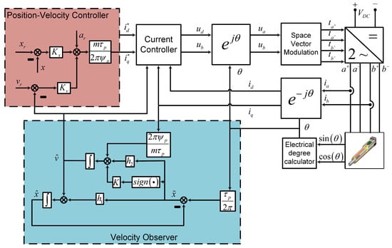
Figure 3. The proposed control scheme of polysolenoid linear motor.

5. Numerical Simulation

The Polysolenoid Linear Motor’s parameters use in this simulation are listed in Table 1. The parameters are selected from LinMot industrial PLM (P01-23x80/80x140). This motor is packed with two position sensors which release $sin\left(\theta \right)$ and $cos\left(\theta \right)$ for flux oriented control (FOC). To verify the effectiveness of the proposed method, the simulation includes two scenarios. The first one demonstrates the performance of the proposed controllers and observer in the case where measurement noises are excluded. While the other one focuses on the impacts of measurement noise in the position feedback signal. Both of them share the same controller, observer, and disturbance load.

Table 1. Parameters of the Polysolenoid Linear Motor (PLM).

Parameter	Notation	Value	Unit
Phase resistance	$R_s$	10.3	ohm
Slider (rotor) mass	m	0.171	kg
Phase inductance	$L_a,L_b$	1.4	mH
Pairs of poles	$n_p$	1
Pole pitch	$\tau$	10	mm
Flux	${\psi }_p$	0.035	Wb

MATLAB/Simulink models of the observer-based tracking control for PLM drive system are built with sampling time ${10}^{-5}$ s. The disturbance load used in the simulations is chosen as: $f_{\ell }\left(t\right)=3+\frac{16}{\pi }sin\left(20t\right)+\frac{16}{3\pi }sin\left(60t\right)+\frac{16}{5\pi }sin\left(100t\right)$. Practically, it should be noted that $f_m\left(t\right)$ is very small in comparison with $f_{\ell }\left(t\right)$. As a result, we select $\overline{F}=60,\overline{\delta F}=2000$. From (10) and (11), parameters of observer (8) are give by $K=100$, $h_1={10}^3$, $h_2={2\times 10}^4$, $\alpha =30$, $\gamma =0.1$. In addition, (27), (28) and (29) result in the position and current controller parameters: $K_p={10}^5$, $K_v={2\times 10}^3,K_d=K_p=10,K_{id}=K_{iq}={10}^4$.

5.1. Simulation Results in Case of None Measurement Noise

In this scenario, we assume that the position sensor is accurate, the initial observer errors are selected as $\tilde{x}\left(0\right)=0$ and $\tilde{v}\left(0\right)=0.1$. As can be seen in Figure 4, position, and velocity of PLM track the reference signals. Besides, there are fluctuations in position and velocity error in Figure 4c,d due to the transition of observer error. According to Figure 5c, despite the disturbance load shown in Figure 5d, the observer error still converges to zero in approximately in 0.1 s. During this interval, the motor does not move, which shows our advantage in velocity observer in comparison with other techniques based on EMF. Therefore, the statement in Theorem 1 is verified. Further, the position can be maintained under the impact of disturbance load. The Figure 5c shows that $i_q\left(t\right)$ tracks the reference signal $i_q^{*}$ by current controllers in Section 4.2. The simulated results verify that the PLM observer-based control system under the disturbance load has a high precision and response position.

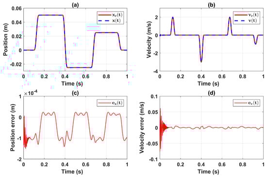
Figure 4. Time response of (a) position tracking; (b) velocity tracking; (c) position error; (d) velocity error.

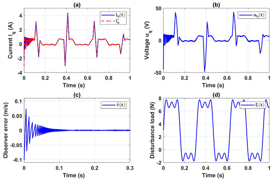
Figure 5. Time behavior of (a) quadrature current; (b) quadrature voltage; (c) velocity observer error; (d) disturbance load.

5.2. Simulation Results in Presence of Measurement Noise

To verify our algorithm, we assume that the position feedback signal is affected by measurement noise as following

$$\begin{array}{c}\hfill x_{meas}\left(t\right)=x\left(t\right)+n\left(t\right)\end{array}$$

(36)

where $x_{meas}\left(t\right)$ is the position feedback signal and $n\left(t\right)$ is a white noise process. In this case, the conventional approaches based on measurement of speed using a position sensor fails to estimate the actual velocity. Due to the measurement noise, the initial observer position $\widehat{x}\left(0\right)$ can not match to initial actual position $x\left(0\right)$. Accordingly, observer errors are selected as $\tilde{x}\left(0\right)={5\times 10}^{-3}$, $\tilde{v}\left(0\right)=0.1$ in the simulation. Figure 6a shows the measurement and actual position. With this measurement signal, the conventional approach which uses low-pass filter and derivatives can not estimated velocity. Overall, our control method still has merits in position tracking control, as presented in Figure 6c,d. As can be seen in Figure 7c,d, the observer errors remain small values after 0.1 s.

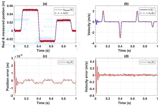
Figure 6. Effects of noise measurement in time response of (a) position tracking; (b) velocity tracking; (c) position error; (d) velocity error.

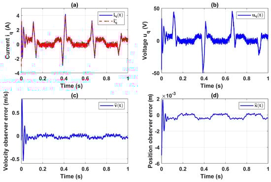
Figure 7. Effects of noise measurement in time behavior of (a) quadrature current, (b) quadrature voltage, (c) velocity observer error and (d) position observer error.

6. Conclusions

This paper has addressed tracking control problems of PLM with velocity sensorless and unknown disturbance force. The key success in our approach has laid on a novel observer, which guarantees asymptotic convergence of the observer errors. Further, the observer can provide estate estimation in the presence of unknown disturbance, and also deal with measurement noises. In cooperation with observed velocity, the position-velocity and current tracking controllers have been designed by using the Lyapunov direct method, such that the tracking error converges to arbitrarily small values by adjusting control parameters. Accordingly, the stability analysis has been presented religiously to enhance the reliability of our results. As a result, this study has possibly proposed a method to overcomes some drawbacks of existed studies on velocity-sensorless control. Our future works will focus on a problem of lack of current sensors, with the aim of no further sensor required in the control of PLM.

References

- Gieras, J.F.; Piech, Z.J.; Tomczuk, B. Linear Synchronous Motors: Transportation and Automation Systems; CRC Press: Boca Raton, FL, USA, 2018. [Google Scholar]
- Wang, Y.; Yu, H.; Che, Z.; Wang, Y.; Zeng, C. Extended state observer-based predictive speed control for permanent magnet linear synchronous motor. Processes 2019, 7, 618. [Google Scholar] [CrossRef]
- Wen, T.; Xiang, B.; Wang, Z.; Zhang, S. Speed control of segmented PMLSM based on improved SMC and speed compensation model. Energies 2020, 13, 981. [Google Scholar] [CrossRef]
- Díaz-Pérez, L.; Torralba, M.; Albajez, J.A.; Yagüe-Fabra, J.A. 2D positioning control system for the planar motion of a nanopositioning platform. Appl. Sci. 2019, 9, 4860. [Google Scholar] [CrossRef]
- Wang, W.; Lu, Z.; Hua, W.; Wang, Z.; Cheng, M. Simplified model predictive current control of primary permanent-magnet linear motor traction systems for subway applications. Energies 2019, 12, 4144. [Google Scholar] [CrossRef]
- Tran, M.S.; Hwang, S.J. Design and experiment of a moving magnet actuator based jetting dispenser. Appl. Sci. 2019, 9, 2911. [Google Scholar] [CrossRef]
- Ausderau, D. Polysolenoid-Linearantrieb Mit Genutetem Stator. Ph.D. Thesis, ETH Zurich, Zurich, Switzerland, 2004. [Google Scholar]
- Boldea, I. Linear Electric Machines, Drives, and MAGLEVs Handbook; CRC Press: Boca Raton, FL, USA, 2017. [Google Scholar]
- Quang, N.H.; Quang, N.P.; Hien, N.N.; Binh, N.T. Min max model predictive control for polysolenoid linear motor. Int. J. Power Electr. Drive Syst. ISSN 2018, 2088, 1667. [Google Scholar] [CrossRef]
- Nguyen, H.Q.; Nguyen, P.Q.; Nam, D.P.; Nguyen, T.B. Multi parametric model predictive control based on laguerre model for permanent magnet linear synchronous motors. Int. J. Electr. Comput. Eng. 2019, 9, 1067. [Google Scholar]
- Nguyen, Q.H.; Dao, N.P.; Nguyen, T.T.; Nguyen, H.M.; Nguyen, H.N.; Vu, T.D. Flatness based control structure for polysolenoid permanent stimulation linear motors. Int. J. Electr. Electron. Eng. 2016, 3, 31–37. [Google Scholar]
- Wang, Z.; Hu, C.; Zhu, Y.; He, S.; Yang, K.; Zhang, M. Neural network learning adaptive robust control of an industrial linear motor-driven stage with disturbance rejection ability. IEEE Trans. Ind. Inf. 2017, 13, 2172–2183. [Google Scholar] [CrossRef]
- Ahn, H.S.; Chen, Y.; Dou, H. State-Periodic Adaptive Compensation of Cogging and Coulomb Friction in Permanent Magnet Linear Motors. In Proceedings of the 2005 American Control Conference, Portland, OR, USA, 8–10 June 2005; pp. 3036–3041. [Google Scholar]
- Tan, K.; Huang, S.; Lee, T. Robust adaptive numerical compensation for friction and force ripple in permanent-magnet linear motors. IEEE Trans. Magn. 2002, 38, 221–228. [Google Scholar] [CrossRef]
- Zhang, D.; Chen, Y.; Zhou, Z.; Ai, W.; Li, X. Robust adaptive motion control of permanent magnet linear motors based on disturbance compensation. IET Electr. Power Appl. 2007, 1, 543–548. [Google Scholar] [CrossRef]
- Sun, G.; Wu, L.; Kuang, Z.; Ma, Z.; Liu, J. Practical tracking control of linear motor via fractional-order sliding mode. Automatica 2018, 94, 221–235. [Google Scholar] [CrossRef]
- Du, H.; Chen, X.; Wen, G.; Yu, X.; Lü, J. Discrete-time fast terminal sliding mode control for permanent magnet linear motor. IEEE Trans. Ind. Electron. 2018, 65, 9916–9927. [Google Scholar] [CrossRef]
- Sun, G.; Ma, Z. Practical tracking control of linear motor with adaptive fractional order terminal sliding mode control. IEEE/ASME Trans. Mechatron. 2017, 22, 2643–2653. [Google Scholar] [CrossRef]
- Cupertino, F.; Giangrande, P.; Pellegrino, G.; Salvatore, L. End effects in linear tubular motors and compensated position sensorless control based on pulsating voltage injection. IEEE Trans. Ind. Electron. 2010, 58, 494–502. [Google Scholar] [CrossRef]
- Hussain, H.A.; Toliyat, H.A. Back-EMF Based Sensorless Vector Control of Tubular PM Linear Motors. In Proceedings of the 2015 IEEE International Electric Machines & Drives Conference (IEMDC), Coeur d’Alene, ID, USA, 10–13 May 2015; pp. 878–883. [Google Scholar]
- Giangrande, P.; Cupertino, F.; Pellegrino, G. Modelling of Linear Motor End-Effects for Saliency Based Sensorless Control. In Proceedings of the 2010 IEEE Energy Conversion Congress and Exposition, Atlanta, GA, USA, 12–16 September 2010; pp. 3261–3268. [Google Scholar]
- Accetta, A.; Cirrincione, M.; Pucci, M.; Vitale, G. Neural sensorless control of linear induction motors by a full-order Luenberger observer considering the end effects. IEEE Trans. Ind. Appl. 2013, 50, 1891–1904. [Google Scholar] [CrossRef]
- Yu, P.-Q.; Lu, Y.-H.; Wang, Y.; Yang, W.-M.; Chen, Z.-C. Research on permanent magnet linear synchronous motor position sensorless control system. Proc. Chin. Soc. Electr. Eng. 2007, 27, 53–57. [Google Scholar]
- Cupertino, F.; Pellegrino, G.; Giangrande, P.; Salvatore, L. Sensorless position control of permanent-magnet motors with pulsating current injection and compensation of motor end effects. IEEE Trans. Ind. Appl. 2011, 47, 1371–1379. [Google Scholar] [CrossRef]
- Holtz, J. Sensorless control of induction machines—With or without signal injection? IEEE Trans. Ind. Electron. 2006, 53, 7–30. [Google Scholar] [CrossRef]
- Silva, C.; Asher, G.M.; Sumner, M. Hybrid rotor position observer for wide speed-range sensorless PM motor drives including zero speed. IEEE Trans. Ind. Electron. 2006, 53, 373–378. [Google Scholar] [CrossRef]
- LinMot Company Home Page: Products, Linear Motors. Available online: https://linmot.com/products/linear-motors/ (accessed on 1 March 2020).
- Lim, K.C.; Woo, J.K.; Kang, G.H.; Hong, J.P.; Kim, G.T. Detent force minimization techniques in permanent magnet linear synchronous motors. IEEE Trans. Magn. 2002, 38, 1157–1160. [Google Scholar]
- Zhao, W.; Jiao, S.; Chen, Q.; Xu, D.; Ji, J. Sensorless control of a linear permanent-magnet motor based on an improved disturbance observer. IEEE Trans. Ind. Electron. 2018, 65, 9291–9300. [Google Scholar] [CrossRef]
- Khalil, H.K.; Grizzle, J.W. Nonlinear Systems; Prentice Hall: Upper Saddle River, NJ, USA, 2002; Volume 3. [Google Scholar]
- Atassi, A.; Khalil, H. Separation results for the stabilization of nonlinear systems using different high-gain observer designs. Syst. Control Lett. 2000, 39, 183–191. [Google Scholar] [CrossRef]
- Peng, C.-C.; Li, Y.; Chen, C.-L. A robust integral type backstepping controller design for control of uncertain nonlinear systems subject to disturbance. Int. J. Innov. Comput. Inf. Control 2011, 7, 2543–2560. [Google Scholar]
- Peng, C.-C. Nonlinear integral type observer design for state estimation and unknown input reconstruction. Appl. Sci. 2017, 7, 67. [Google Scholar] [CrossRef]
© 2020 by the author. Licensee MDPI, Basel, Switzerland. This article is an open access article distributed under the terms and conditions of the Creative Commons Attribution (CC BY) license (http://creativecommons.org/licenses/by/4.0/).