1. Introduction
An electromagnetic launcher (EML) is a system which uses electricity to propel a projectile [
1]. A coil gun is a type of EML which has the ability to launch magnetic objects (such as iron rods) by converting electrical energy into kinetic energy using a coil [
2].
Launching non-magnetic objects cannot be achieved using coil guns directly because these objects are not affected by the magnetic field; however, it can be done with an “indirect coil gun”, using a magnetic plunger accelerated by a coil, which propels the non-magnetic object by continuous contact or elastic shock. Both these propelling techniques can be combined in a multi-phase EML. The optimization of this type of launcher is the purpose of this work. More precisely, the initial position of the plunger and the length of the non-magnetic plunger extension have an important effect on the launching sequence and its efficiency. A method for optimizing these two parameters is proposed in this paper, which can easily be adapted to any other indirect coil gun.
To illustrate our method, we have chosen to optimize a kicking system used at the RoboCup in the Middle Size League, which is a robot soccer competition where the robots have a limited size and weight in which to embed a soccer ball launching systems. This article is divided into three parts:
In
Section 2, the principles of coil guns are presented with limitations concerning their modeling;
In
Section 3, a mechanic and electromagnetic model is proposed and implemented using finite elements simulation tools for the electromagnetic part of the coil gun, and using Matlab Simulink for the mechanical and electrical aspects;
In
Section 4, the simulation results are discussed in order to optimize the parameters of an existing indirect coil gun.
The RoboCup is an international competition where robot teams play soccer. One of the objectives of the competition is for one of the robot teams to have won against a professional, human soccer team by 2050. In the Middle Size League (MSL), teams are composed of five robots playing autonomously on a 22 m by 14 m soccer field with a real soccer ball (diameter 22 cm) weighting 450 g. Each robot has a maximum length of 52 cm, a maximum width of 52 cm, and a maximum height of 80 cm. Current kicking systems used in the MSL have the ability of propelling balls with a speed of 12 m s. This speed is respectable and allows them to kick balls at a distance of 15 m, but this is limited when compared with real soccer players.
In order to make a comparison, a shot from a professional soccer player can reach 130 km h, compared with 43 km h for current MSL robots. In terms of kinetic energy, = 32 J is transmitted to the ball at the RoboCup, compared to = 300 J transmitted by a real professional player. The difference between them is about a factor of 10, showing that an important step has to be made if the robots are to compete with humans.
The RoboCup MSL case study has been chosen due to the relevance of the trade-off regarding the optimization of the speed of the ball being kicked by the indirect coil gun and the strict size constraints in the competition rules. RoboCup robots need compact but powerful coil guns. Existing systems, able to strike a ball at 12 m s
, have an acceleration of about 100 g and a strike time of about 20 ms. As shown in
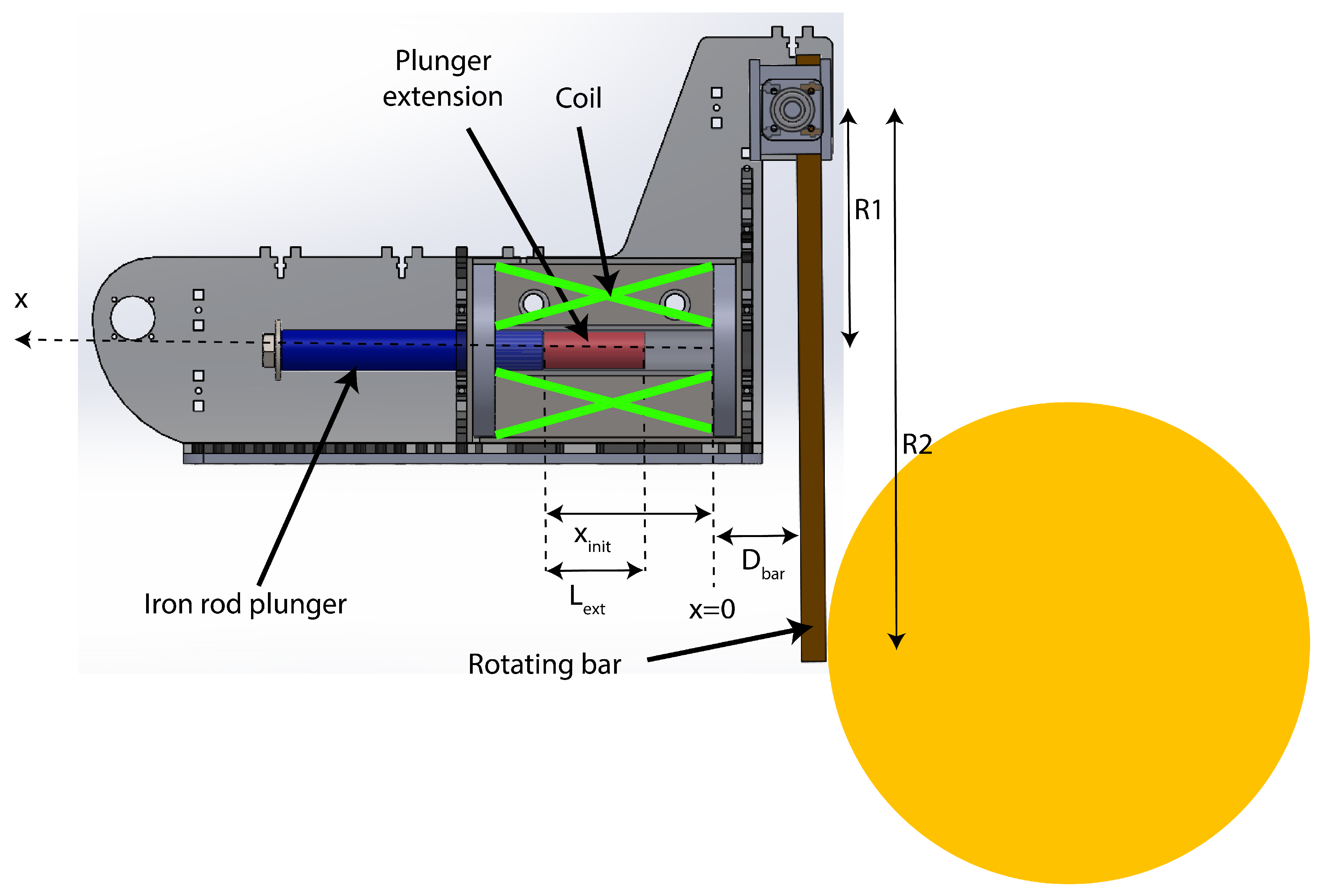
Figure 1, the size of the whole kicking system, including the indirect coil gun, is about 30 cm including the coil and the iron rod, with a coil size of about 10 cm to 12 cm in length, a rod size of about 13 cm in length, and a rod stroke of about 12 cm.
2. Principles of Coil Guns
2.1. Physical Concept
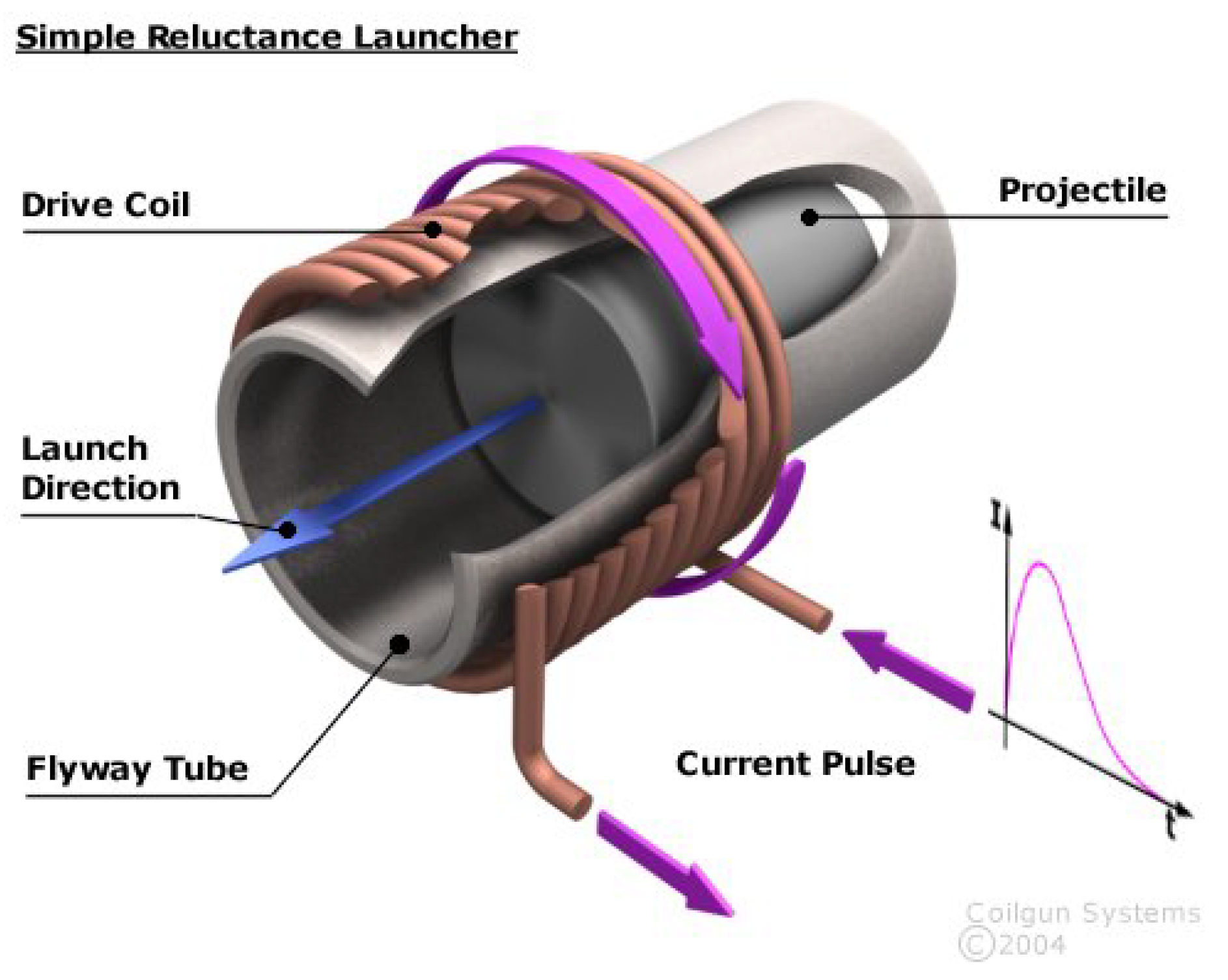
Coil guns are made using a variable reluctance magnetic circuit composed of a fixed magnetic circuit looped by a magnetic iron projectile. A coil is placed around the stroke of the iron rod in order to magnetize the magnetic circuit and to create a magnetic force on the rod.
Considering that the magnetic field in a magnetic circuit tends to be maximized where possible, the air gap in a magnetic circuit tends to be reduced, resulting in a force on the rod, propelling it when the magnetic circuit is excited with a coil current pulse, as shown in
Figure 2. This is the principle of a variable reluctance actuator.
In our case study, a large capacitor (4700 F) is discharged in the coil in order to produce a high current generating the magnetic field and force. A mobile plunger (iron rod) is able to move in this field, sliding in a stainless steel tube. The iron rod is attracted to the centre of the stainless steel tube and thus accelerated until it reaches this point. It can be slowed down if the plunger goes over this point while the current in the coil is still present, but this does not happen in real conditions, as is shown later.
Current discharge on the coil can be described by a second order differential equation, but having non-constant coefficients because of the changing value of the inductor over time. In this paper, we propose an electrical model taking into account the variation of the inductance when the iron rod slides forward in the coil.
2.2. Electromagnetic Theory and Simulation Software
The Hopkinson law is the foundation of variable reluctance actuators: , where:
Consequently, magnetic flux is equal to and coil force is equal to with , where S is the surface of one coil turn, and the normal vector to the coil.
Going deeper into a theoretical electrical model is interesting if the reluctance is constant, in order to find an analytical solution. However, there are two main factors making it non-constant: the first one is the position of the plunger, and the second is the saturation of the magnetic circuit [
3], as shown in
Figure 3, which can be very important if the coil current is high. In order to take these non-linearities into account, a finite-element model-based simulator was used for calculating the force and the inductance values under different conditions [
4]. The open source software used was
FEMM 4.2, programmed by D.C. Meeker.
FEMM 4.2 approximates the values of
at any place in the system for each plunger and current combination. Numerical computation is performed in a static way, meaning that the kicking system evolution can be considered as a succession of short time independent magneto-static problems. For each of these problems, the following equations link magnetic field intensity
B and magnetic excitation
H:
and
can be linked together in a linear approach:
or in a more realistic non-linear approach:
FEMM software tries to find a field that satisfies the linear approach and the flux density equation with the magnetic vector potential
defined as
can be found by the software using Equation (
4) with a conjugate gradient method, so we can rewrite Equation (
1) as
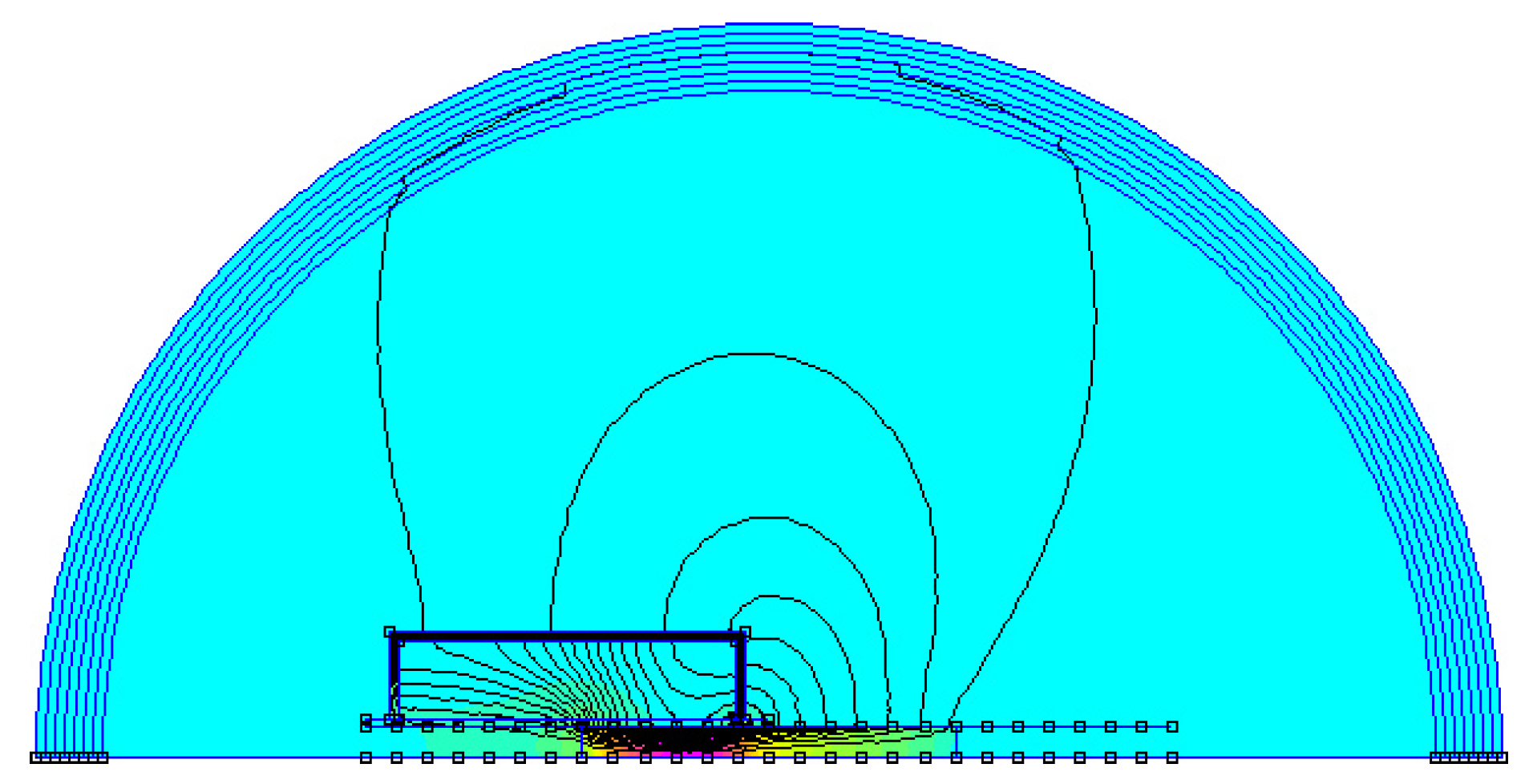
Using this equation, the software calculates
and
in every place of the EML, as shown in
Figure 4. This computation is done using a successive approximation finite element solver on an axisymmetric model with a spherical boundary. Mesh is determined using an heuristic with the following characteristics: a maximum allowable mesh size is computed as
of the length of the diagonal of the bounding box of any region, leading to the generation of a default mesh with about 4200 elements in an empty square region, as shown in
Figure 5. Fine meshing is also forced into all the corners and a 5 degree default discretization is used for arc segments.
FEMM 4.2 also evaluates integral values in a specific part of the system such as the inductance of the coil or the force applied on the iron plunger. This kind of computation takes about 2 seconds on a standard Intel Core I7 processor. To go further, it can be automated using a LUA script for evaluating force and inductance for different currents and positions of the plunger.
2.3. Electrical Model
The coil gun inductance
L is powered by a pre-loaded high value and voltage (i.e., 4700
F, 450 V) capacitor
C, switched by an Insulated Gate Bipolar Transistor (IGBT), as shown in
Figure 6. Resistor
R has to be taken into account considering the high number of loops of the coil, it can be measured or calculated using
where
is the resistivity of copper,
L the length of the coil wire, and
S the surface of a wire section. This leads to the differential Equation (
7).
This equation can be solved easily when
L,
C, and
R are constants; however,
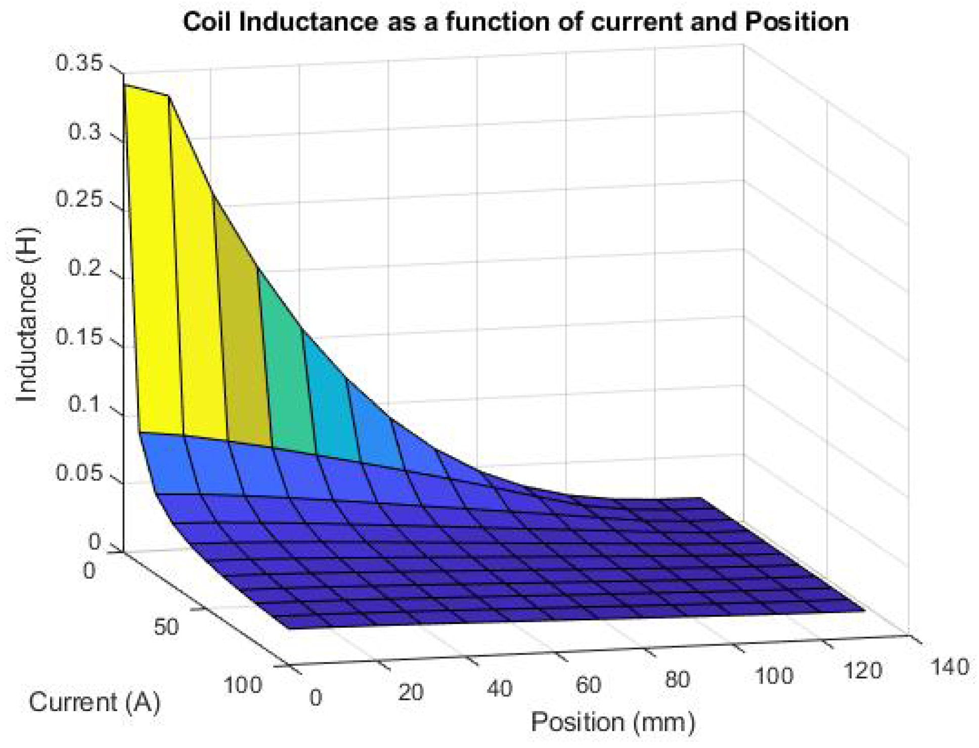
L is not constant in our case. As shown in
Figure 7, simulations on
FEMM 4.2 using a
LUA script show that the
L inductance value can vary by a factor of 18 in our case study, going from 19 mH to 342 mH for the same coil depending on the plunger position and on the coil current. Discrete values of the inductance are calculated for positions (as shown in
Figure 1) of the plunger varying from x = 0 mm to 130 mm by increment of 10 mm, and for coil currents varying from
to
by increment of
as shown in
Table 1.
When the plunger is outside the coil and when the current is high, the inductance has the lowest values. When the plunger is in the centre of the coil and when current is low, the magnetic field is well guided and magnetic materials are not saturated, leading to a high inductance value.
2.4. Mechanical Model
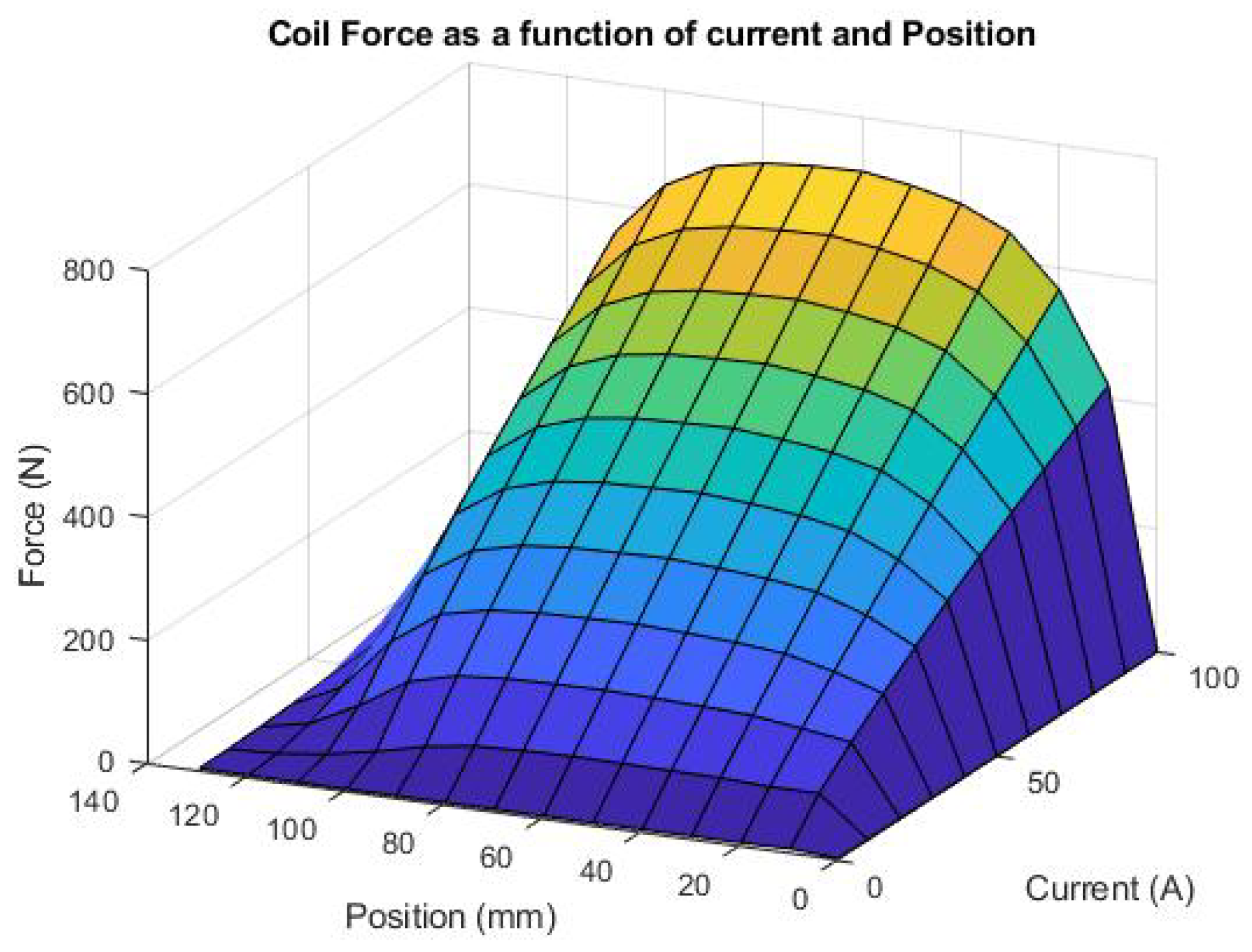
As explained before, force on the plunger cannot be calculated analytically. Simulations using
FEMM 4.2 combined with a LUA script show (
Figure 8) that force varies in our case study from 0 N to 850 N for the same coil depending on the plunger position and on the coil current. Discrete values of the force are calculated for positions (as shown in
Figure 1) of the plunger varying from x = 0 mm to 130 mm by increment of 10 mm, and for coil currents varying from 0 A to 100 A by an increment of 10 A, as shown in
Table 2.
When the plunger is outside the coil, the force is very small. This is due to the importance of the air gap related to the absence of the plunger for looping back the magnetic circuit. When the plunger is exactly in the centre of the coil, force is null for any value of the current because magnetic flux is maximal. The maximal force strength is obtained for high currents and plunger positions between 40 mm and 80 mm from the centre of the coil.
3. Mixed Electrical and Mechanical Model of the Indirect Coil Gun
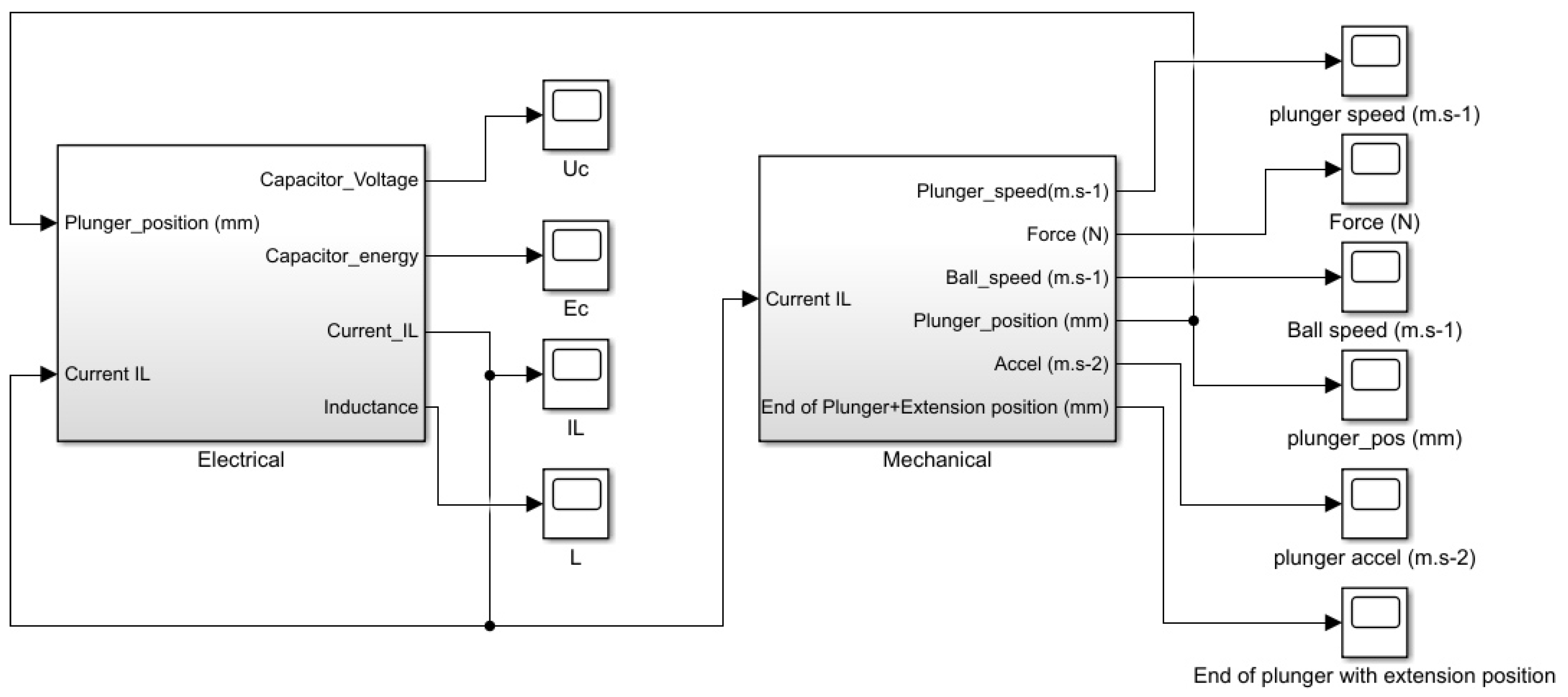
Inductance and magnetic force values are necessary to build a model of the coil gun for simulating it precisely. Calculated using FEMM 4.2, they are implemented using look-up tables, taking into account the plunger position and coil current in order to approximate inductance and force for every configuration of the system.
For this mechatronic model combining mechanic, electric, and magnetic modeling, the Matlab Simulink tool was used, as shown in
Figure 9.
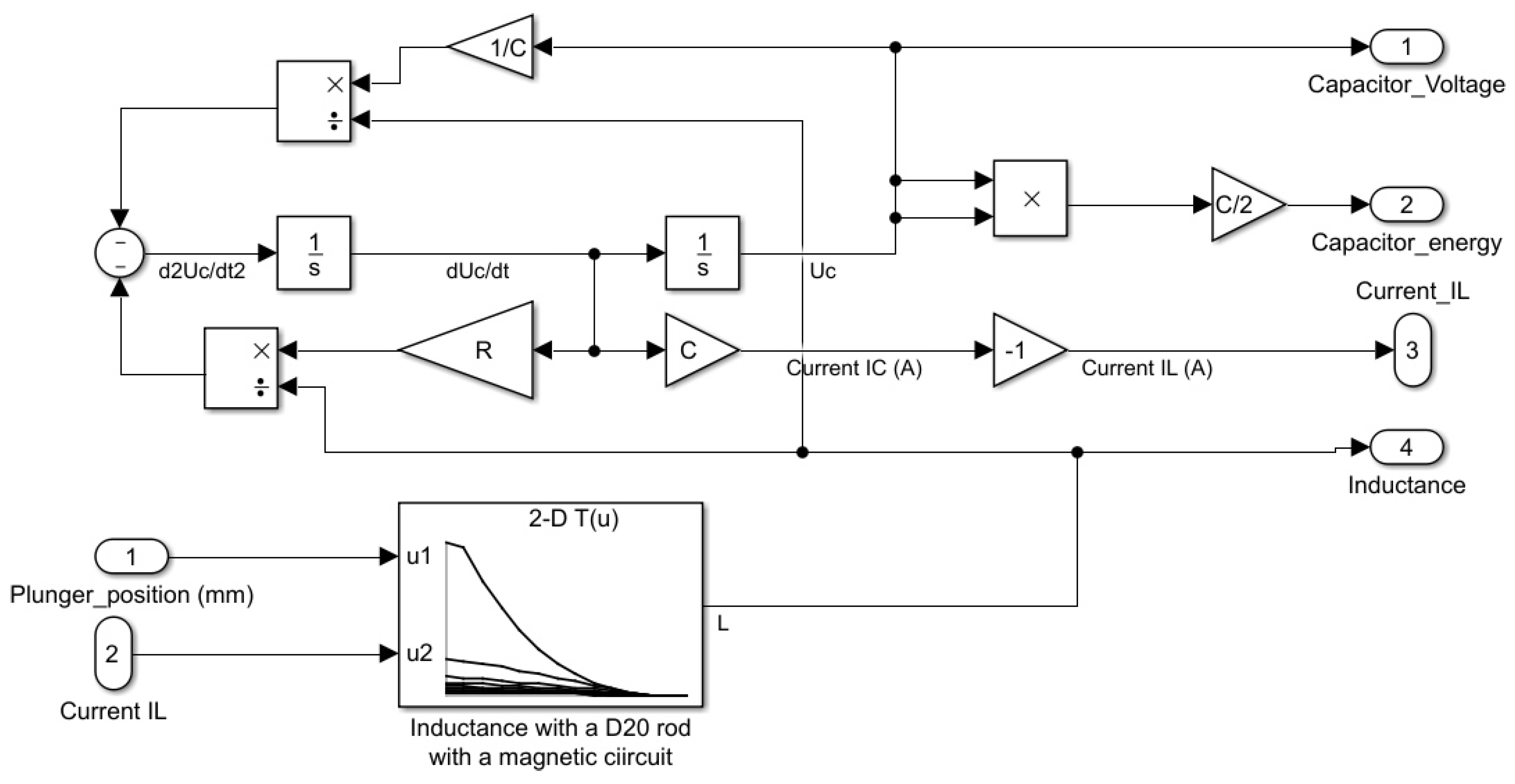
3.1. Electrical Model
The electrical part is described in
Figure 10. It implements the electrical differential Equation (
7) using discrete blocks. This is necessary because coefficients of the equation are not constant because of the dependence of inductance
L on the current and the position of the plunger.
As said before, this dependence is modeled using a look-up table (LUT), interpolating linearly the value of L using the simulations performed with FEMM 4.2.
3.2. Mechanical Model
The indirect coil gun mechanical system used for kicking balls is described in
Figure 1.
This model is not simple because the plunger hits an aluminum lever at a distance
from its rotation centre in order to transmit movement to the ball. Thus, the movement can be split into three phases, as shown in
Figure 11.
Phase 1: the plunger is accelerated without contact on the lever. Acceleration is caused by the magnetic force only, as shown in Equation (
8). Force
is a function of the plunger position and current
I. Again, this dependence is modeled using an LUT interpolating linearly the value of
F using the simulations performed with
FEMM 4.2.
Phase 2: an elastic shock occurs when plunger hits the lever. Kinetic energy is conserved as described in Equation (
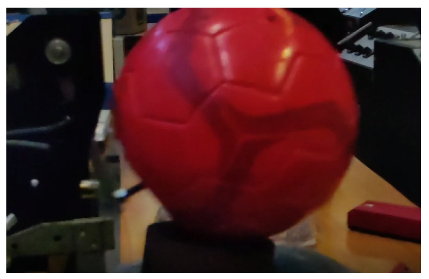
9). In theory, the speeds of the ball, lever, and plunger are not equal after the shock, but in reality they are all moving together thanks to the deformation of the ball which ensures that the contact is permanent after the shock, as shown in the slow motion picture in
Figure 12.
where
is the inertial moment of the lever,
and
are the distances between the lever axis and the plunger impact point and the ball impact point, respectively, as shown in
Figure 1.
This leads to a plunger speed just after the shock equal to the
, given in Equation (
10).
Phase 3: plunger is accelerated in contact with the lever, which one is also in contact with the ball. This means that the lever applies a force on the plunger in subtraction of the magnetic force as shown in Equation (
11). This force is inertial due to the acceleration of the ball and the lever, as shown in Equation (
12).
where
with
For small
angles,
, this leads to
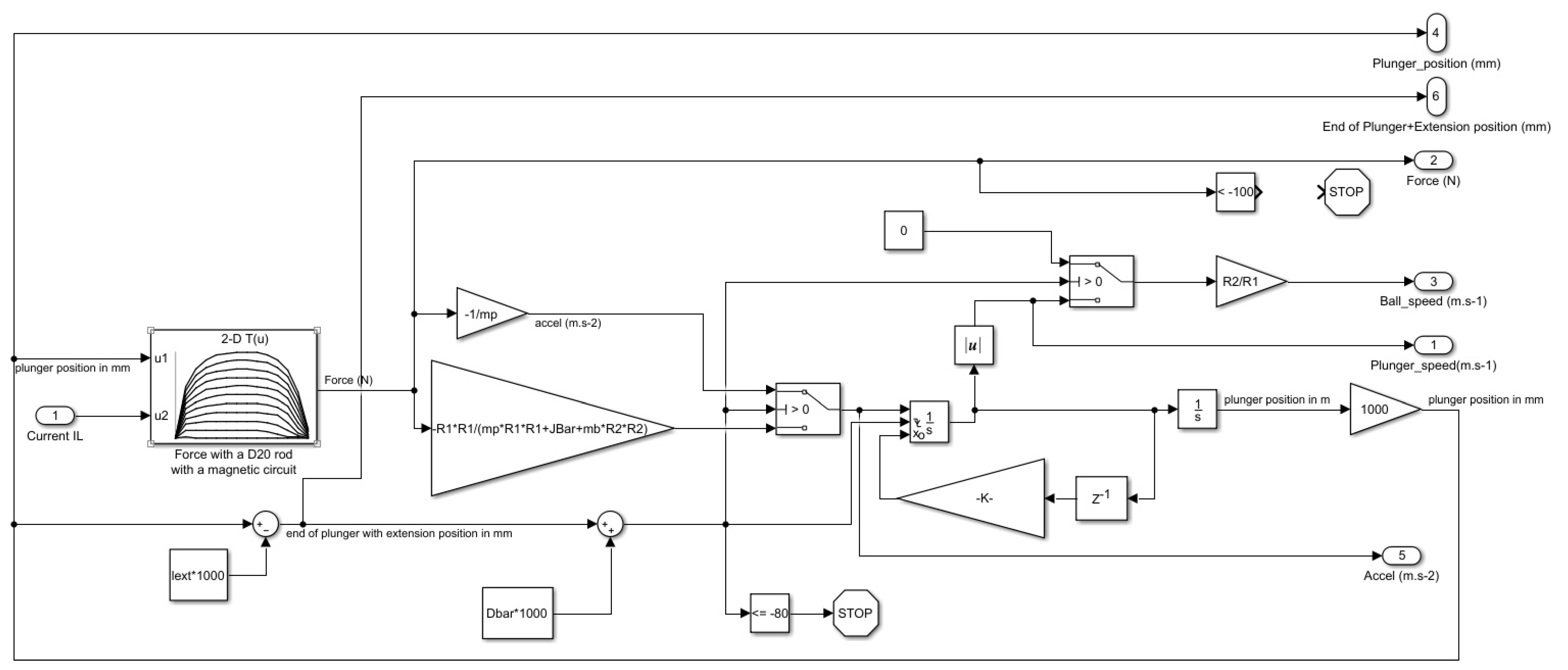
This mechanical model is implemented with Matlab Simulink using discrete blocks and switches for simulating the different phases of the movement, as shown in
Figure 13.
4. Indirect Coil Gun Simulation Results
The indirect coil gun system presented here and used in the robots at the RoboCup was simulated using Matlab Simulink. Even if the mechanical structure and the electromagnetic properties of the kicking system are completely defined, as in
Figure 1, there are 2 remaining degrees of freedom in order to optimize its power: the initial position
of the plunger and the length
of the non-magnetic extension of the plunger.
In order to compare the results with other previous studies, the kicking system simulated is identical to that of the
Tech United Team described in [
5]. Parameters of the model are the following:
Distance from lever axis to plunger touch point: = 13 cm;
Distance from lever axis to ball touch point: = 24 cm;
Coil length: cm;
Coil number of turns: turns;
Plunger iron rod diameter: mm;
Plunger iron rod length: cm;
Plunger iron rod mass: g;
Plunger extension diameter: mm;
Plunger extension length: cm;
Plunger extension mass: (in m);
Distance from coil to lever: cm;
Vertical lever mass: g;
Ball mass: g;
Capacitor value: 4700 F;
Capacitor charge voltage: 450 V;
Coil resistance: 2.5 .
Considering these parameters, we can notice that if , the plunger with its extension is not in contact with the lever at the beginning of the movement, and consequently the launch is divided into three phases. In the limit case, where , the movement only has one phase: the third one with the plunger in contact with the lever from the start.
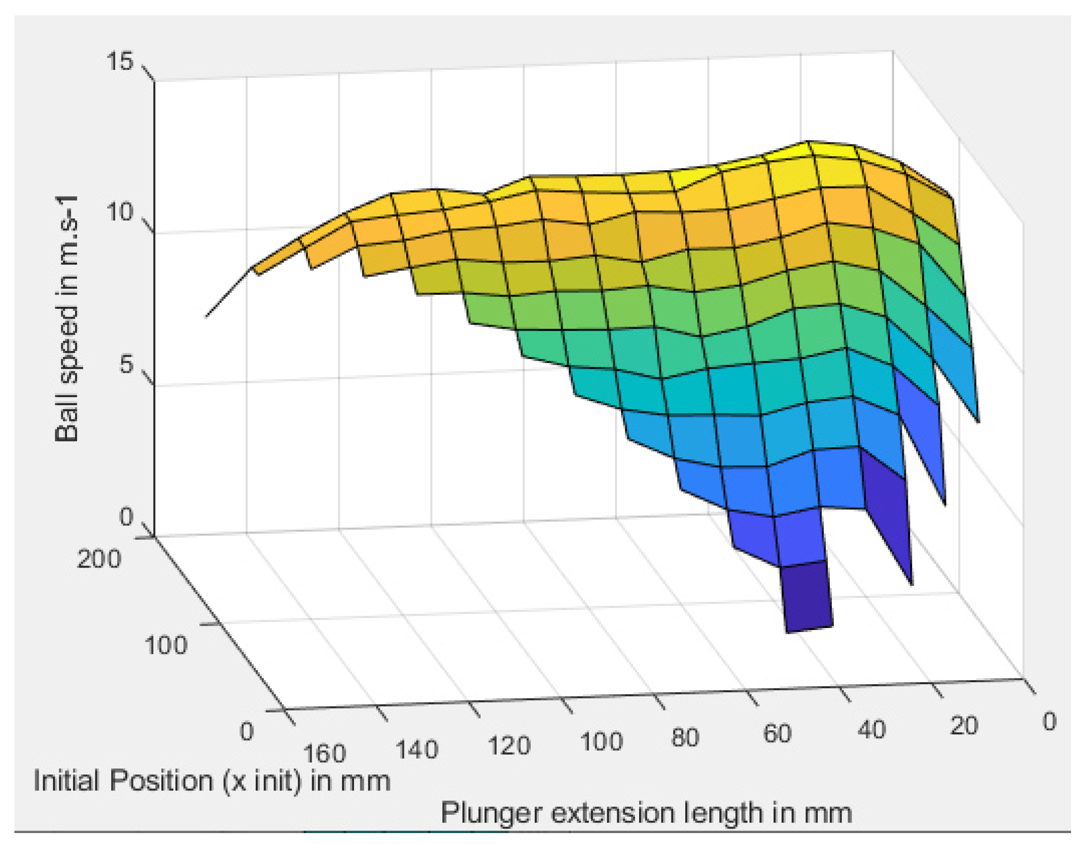
In order to find the best setup corresponding to the highest ball speed, the kicking system was simulated for different values of and chosen as: and . Each simulation took approximately 2 seconds on a Intel Core I7 processor. and were increased manually with an increment of 1 cm.
The results are presented in
Figure 14. The best configuration is to have a plunger initial position of
= 120 mm, and a plunger extension length of
= 30 mm, leading to a ball speed of
= 14.46 m s
. This means that the plunger must be nearly outside the coil at the start and have a short extension of 30 mm only. In this optimal configuration, the movement is a three phase one, with an elastic shock.
Comparison with Previous Experimental Results
In [
5], the
Tech United Team uses the same indirect coil gun structure in a configuration where the plunger with its non-magnetic extension is already touching the lever at the start of the launch. Their case corresponds to
= 110 mm with a plunger extension length of
= 150 mm. The measured ball speed at full switch duty cycle is 11.2 m ([
5] (p. 1664)), compared with 11.1 m s
obtained by our simulation.
Even if the comparison with external samples is too limited, this shows that our model matches very well to the real behavior. It is interesting to note that without changing the mechanical and electromagnetic structure of the coil gun, our optimization leads to a ball speed of 14.46 m s. This speed is higher than the obtained speed, corresponding to more energy transmitted using a three phases movement.
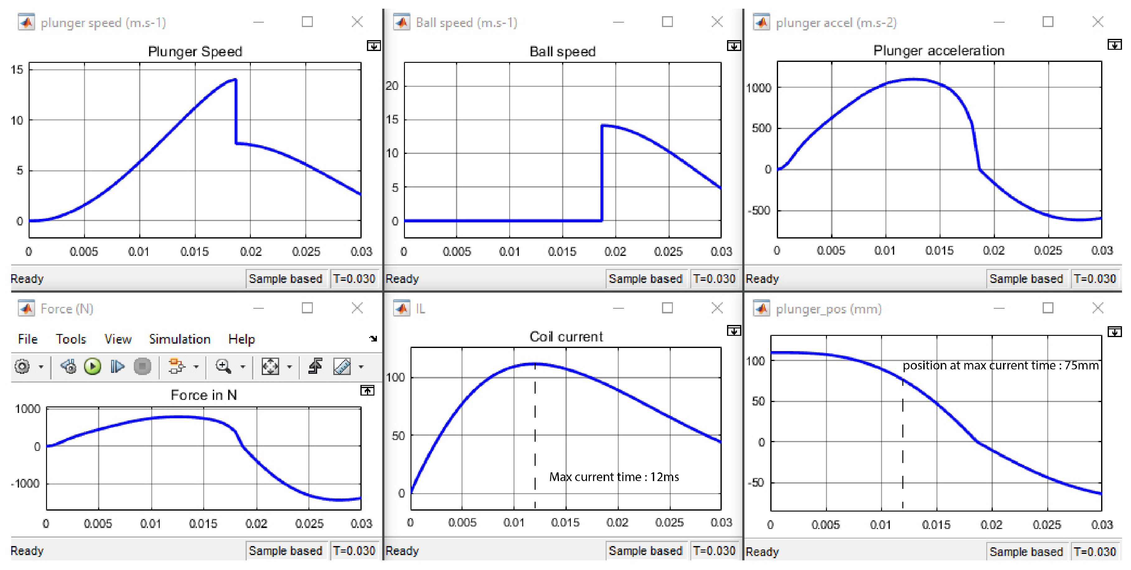
This can be explained by comparing the simulation results. In the optimal case, as shown in
Figure 15, maximum coil current reaches 115 A at
t = 12 ms. The plunger position at this instant is x = 75 mm, optimal for transmitting force to the plunger, as shown in
Figure 8. That means force as a function of position is maximal simultaneously with the current in the coil, leading to an optimal force on the plunger, reaching
N.
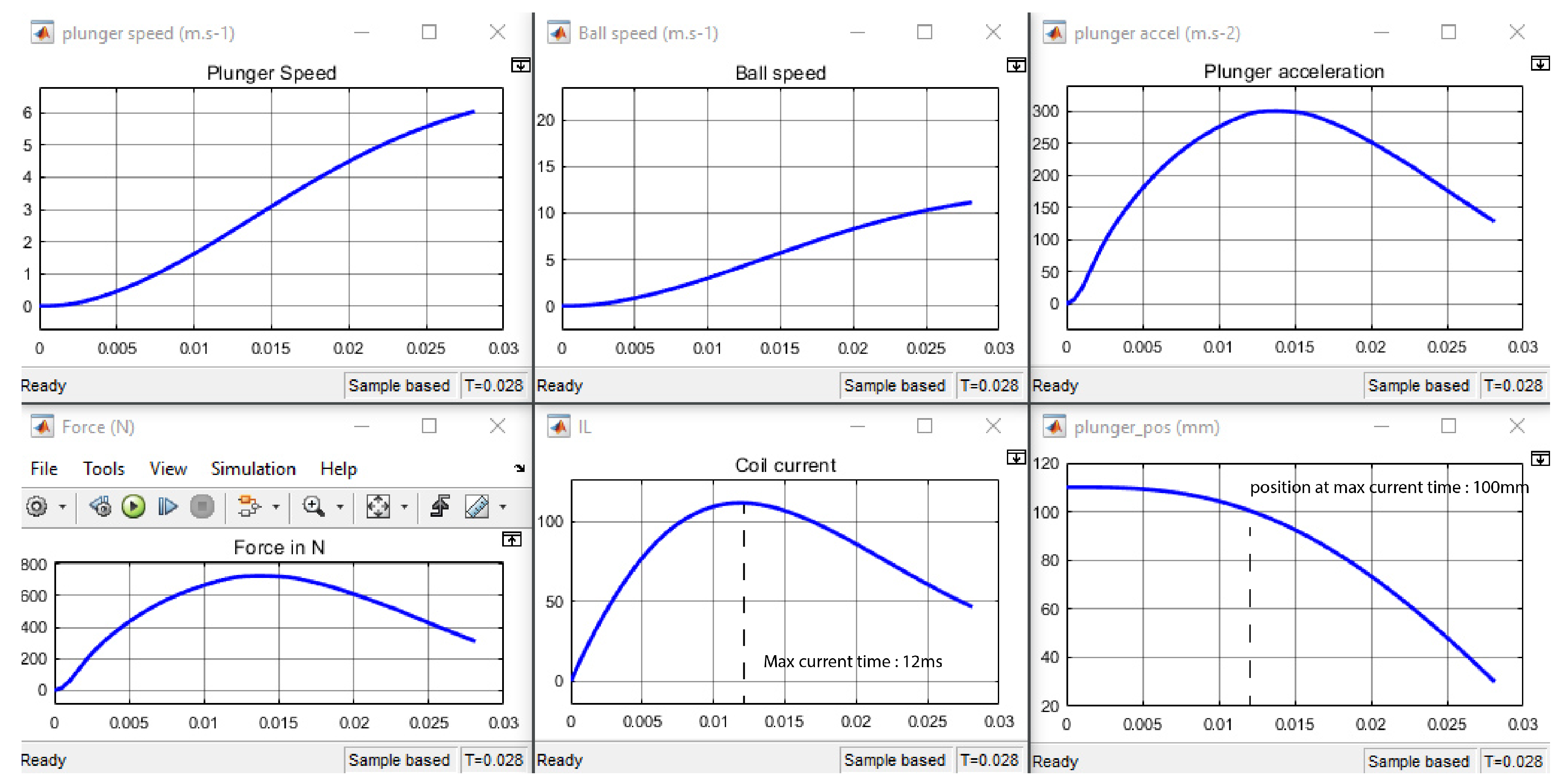
In continuous movement used by the Tech United team, as shown in
Figure 16, the maximum coil current also reaches 115 A at
t = 12 ms. The plunger position at this instant is
x = 100 mm, which is not optimal for transmitting force to the plunger, as shown in
Figure 8. That means force as a function of position is not simultaneously maximal with the current in the coil. Consecutively, force on the plunger only reach
F = 720 N at this time. This delay is due to the fact that the plunger is continuously in contact with the lever and the ball. Thus, acceleration with the ball ≃ 300 m s
is much smaller than without contact ≃ 1100 m s
, leading to a smaller plunger movement when current reach its maximum value.
5. Conclusions
In this paper, we have proposed a method for optimizing indirect coil gun operation. To illustrate our method, we chose to optimize a kicking system used at the RoboCup in the Middle Size League. Firstly, the principles of coil guns were presented, then a mechatronic model, coupling mechanic, electromagnetic, and electric models, was proposed and implemented. In a third part, the simulation results were discussed in order to optimize the parameters of an existing indirect coil gun. This simulator describes for a specific application; however, the method can be easily used to optimize any other indirect coil gun.
In our application, results show that the output speed of the non-magnetic object propelled by the EML can vary a lot depending on the initial configuration of the iron plunger, and depending on the size of its non-magnetic extension. Optimal results are obtained with a three phase propulsion, including an elastic shock. However, this result relies on the assumption that the deformation of the non-magnetic object ensures a permanent contact after the shock. This is a strong hypothesis, but easily valid when the projectile is deformable. Moreover, in the case of a non-deformable contact, the non-magnetic object would have to be very resistant to withstand the very extreme instantaneous acceleration associated with the shock.
In future work, the structure of the coil gun will be optimized, dividing the coil into several smaller coils activated sequentially. For example, scenarios using two, three, or four coils (each one having a half, a third, or a quarter of the total turns of the initial coil) triggered sequentially by software or using a position sensor instead of a single coil, as shown in
Figure 17, will be evaluated as in [
6,
7]. This will lead to having a maximum current on each coil successively when the rod is optimally placed in the coil, leading to an increased projectile speed.


