Article

DNN-Augmented Kinematically Decoupled Three-DoF Origami Parallel Robot for High-Precision Heave and Tilt Control

1
School of Mechanical Engineering, Zhejiang University, Hangzhou 310027, China
2
Zhejiang University Robotics Institute (Yuyao Robotics Research Center), Ningbo 315400, China
*
Author to whom correspondence should be addressed.
Actuators 2025, 14(6), 291; https://doi.org/10.3390/act14060291
Submission received: 13 May 2025 / Revised: 6 June 2025 / Accepted: 12 June 2025 / Published: 13 June 2025
(This article belongs to the Section Actuators for Robotics)

Abstract

This paper presents a three-degrees-of-freedom origami parallel robot that is free from parasitic motion. This robot is designed to achieve one translational and two rotational motions within its workspace, enabling precise orientation about a fixed point—a capability unattainable for parallel robots with parasitic motion. The elimination of parasitic motion is critical, allowing the use of this device in applications requiring high precision. The robot’s key kinematic features include a parasitic motion-free workspace, large orientational capability, compactness, decoupled motion, simplicity in manufacturing and control, mechanically pivoted rotation of the moving platform, and scalability. These characteristics make the robot particularly well-suited for micromanipulation tasks in both manufacturing and medical applications. In manufacturing, it can enable high-precision operations such as micro-assembly, optical fiber alignment, and semiconductor packaging. In medicine, it can support delicate procedures such as microsurgery and cell injection, where sub-micron accuracy, high stability, and precise motion decoupling are critical requirements. The use of nearly identical limbs simplifies the architecture, facilitating easier design, manufacture, and control. The kinematics of the robot is analyzed using reciprocal screw theory for an analytic constraint-embedded Jacobian. To further enhance operational accuracy and robustness, particularly in the presence of uncertainties or disturbances, a deep neural network (DNN)-based state estimation method is integrated, providing accurate forward kinematic predictions. The construction of the robot utilizes origami-inspired limbs and joints, enhancing miniaturization, manufacturing simplicity, and foldability. Although capable of being scaled up or further miniaturized, its current size is 66 mm × 68 mm × 100 mm. The robot’s moving platform is theoretically and experimentally proven to be free of parasitic motion and possesses a large orientation capability. Its unique features are demonstrated, and its potential for high-precision applications is thoroughly discussed.

1. Introduction

Parallel robots (PRs) are prized for their high stiffness, load capacity, and accuracy afforded by closed-loop kinematic chains. However, most lower-degree-of-freedom PRs suffer from parasitic motion—an undesired displacement of the moving platform caused by internal kinematic constraints, which degrades positioning precision and complicates control. The PR architectures illustrated in Figure 1 represent the most common examples that inherently exhibit parasitic motion, stemming from the specific nature of their kinematic constraints. These robots cannot operate properly unless the parasitic motion is correctly modeled and explicitly accounted for in the control strategy. Although structurally important, this motion introduces complexity and inaccuracy, making it undesirable. Traditionally, spherical [1,2], and parallelogram-type [3] mechanisms, or even general six DoF PRs, have been used in scenarios where lower-DoF PRs without parasitic motion would be more suitable. Spherical robots, limited to rotational DoFs, are inadequate for applications requiring heave motion. Their inability to maintain orientation without actuator input also poses manufacturing and assembly challenges. Parallelogram-type robots, restricted to planar movements, require additional actuators and complex design modifications for spatial operation. This leads to an increase in the system’s inertia and also requires more space for both installation and operation. Furthermore, using generic six DoF PRs for tasks requiring fewer DoFs leads to a complicated system control.
This complexity not only makes control more challenging but also heightens the risk of fail-open scenarios, as the system relies solely on software-defined constraints—meaning a software failure could lead to catastrophic consequences. In critical applications like robotic surgery, where heave and tilt motions are essential, it is more reliable to introduce mechanical constraints than to rely solely on software limitations. To address these challenges, researchers have introduced lower-DoF PRs, with 1T2R (one translation and two rotational) motion PRs being widely studied and successfully applied. In 2015, the Starrag Group introduced the Sprint Z3 [4,5] of the Ecospeed series, shown in Figure 1a, a groundbreaking three-degrees-of-freedom parallel robot known for its precision and efficiency in machining, primarily used in aerospace and automotive industries. Its parallel kinematics machining head enabled five-axis simultaneous machining, significantly reducing production times and costs with a maximum cutting volume of up to 8000 cm 3 / min . However, the Sprint Z3 faced a challenge: the presence of parasitic motion, which affected the precision critical to its applications. To mitigate this, an external x(y) bed mechanism was incorporated, adding a layer of complexity to the machine’s control system. Despite this, the Sprint Z3’s success highlighted the importance of 1T2R PRs in precision machining and set new standards in the field. Another interesting application of 1T2R PRs’ reconfigurable surfaces is presented in  [6]. The Ori-Pixel, a Multi-DoFs Origami Pixel, represents a significant advancement in modular reconfigurable surface technology, using an origami-inspired Canfield mechanism [7] to control height, pitch, and roll angles. This versatility enables the Ori-Pixel to render a wider variety of shapes and motion primitives, accurately replicating curved contours, making it suitable for high-precision applications in interactive installations and concept car designs. However, the Ori-Pixel faces the challenge of parasitic motion, leading to gaps between individual pixels to prevent collisions. While these gaps ensure operational safety and reliability, they compromise surface resolution, disrupting the continuity and smoothness of rendered surfaces, particularly in complex and detailed patterns. Thus, while the Ori-Pixel is a significant advance in reconfigurable surface technology, addressing parasitic motion and its impact on surface resolution remains a critical area for further refinement. Many other PRs exhibiting parasitic motion have been designed for a variety of purposes, including the A3 head for high-precision machining, as depicted in Figure 1b, and a satellite thruster used by NASA, shown in Figure 1c, among others. Recognizing parasitic motion as a major drawback in lower-DoF PRs, extensive research has been conducted [8,9,10,11,12]. The literature suggests that developing lower-DoF PRs without parasitic motion is crucial for various applications [9,10,13].

2. Impact of Parasitic Motion in Precision-Dependent Applications

Parasitic motion—unintended displacement of a robot’s moving platform arising from internal structural constraints—can significantly impact precision-critical operations. Such undesired motion complicates control algorithms and heightens the risk of system failures, particularly in applications where real-time corrective measures are limited or impractical.
In minimally invasive surgery (MIS), parasitic motion may cause inadvertent tool deviations, risking unintended tissue damage due to the inherent difficulty of real-time correction. In aerospace contexts, such as satellite tracking, parasitic misalignments degrade communication accuracy and reliability, necessitating complex additional correction hardware or software.
Across diverse high-precision fields, parasitic motion can seriously compromise system effectiveness by reducing accuracy, reliability, and overall performance. The following specific applications exemplify the severe implications of parasitic motion:
  • Pointing and Satellite Tracking Systems: Precise angular alignment is critical for effective satellite communication. Parasitic motion introduces alignment errors, potentially causing signal attenuation or loss.
  • Satellite Thrust Generators: Accurate thrust vectoring ensures correct orbital maneuvers. Parasitic-induced misalignment may cause off-axis thrust, resulting in incorrect maneuvers and increased collision risks.
  • High-Precision Machining Systems: CNC and ultra-precision machining demand accurate tool paths. Parasitic motion leads to surface defects, dimensional inaccuracies, and potential damage to tools or workpieces.
  • Coordinate Measuring Machines (CMMs): Accurate probe positioning is vital for geometric assessments. Parasitic motion compromises measurement integrity, leading to erroneous evaluations and product rejections.
  • Interactive and Reconfigurable Surfaces: Adaptive interfaces and tactile displays rely on continuous, uniform responses. Parasitic motion disrupts continuity, adversely affecting responsiveness and user experience.
  • Haptic VR Controllers: Realistic tactile feedback in virtual environments demands precise motion control. Parasitic motion causes discrepancies between visual and haptic cues, diminishing user immersion and realism.
  • Sun Tracking Mechanisms: Optimal solar energy capture necessitates accurate tracking of the sun’s position. Parasitic misalignments reduce exposure, diminishing overall energy efficiency.
These examples highlight that the mitigation of parasitic motion is essential to maintaining system precision, reliability, and operational effectiveness. Computational analyses further illustrate this impact. For instance, computing the parasitic motion amplitude of the 3-Revolute–Spherical–Revolute (3-RSR) parallel robot (Figure 1c), reveals significant translational deviations along the x and y axes, and rotational deviations about the z axis, as shown in Figure 2. Even structurally symmetrical lower-degrees-of-freedom parallel robots thus exhibit notable parasitic motion, underscoring the necessity for targeted design and control strategies to effectively eliminate or reduce such deviations.
To overcome the limitations imposed by parasitic motion, several research efforts have studied parasitic motion and investigated spatial PRs with reduced DoFs specifically designed to eliminate such effects [9,10,11,12,13,14,15,16,17,18]. In particular, robots providing one translational and two rotational motions without parasitic motion have received considerable attention due to their relevance in applications demanding precise orientation and positioning [12].
Although previously proposed robots satisfy non-parasitic 1T2R motion at the end-effector, some have non-identical limbs with complex architectures [2,13], which introduce manufacturing and assembly difficulties. At the same time, some still comprise parasitic motion, at least in one of the constraint directions [9], causing inaccuracy and control difficulty. Additionally, existing robots that are free of parasitic motion employ linear actuators [17]. This increases the overall volume of the robot, hindering its simplicity and compactness, particularly for applications such as surgery and space exploration. In 2012, Kuo et al. introduced a fully decoupled 1T2R robot for surgical applications [2]. Due to the decoupled DoFs, the device allows pivoting at the incision point, which ensures surgical safety. However, each limb is built with an excessive and wide variety of kinematic joints. Seo et al. have also developed a six-DoF robot-assisted untact Swab sampling robot for COVID-19 and similar tests [19]. However, these kinds of applications require only three DoFs. The remaining DoFs are used to avoid parasitic motion and singularities. It should be noted that using higher-DoF robots for tasks requiring fewer degrees of freedom is expensive in terms of both cost and control. Moreover, it is not fail-safe if an error occurs in the control software or from the doctors’ fatigue during the surgical process, since limiting the DoFs is entirely software-dependent.
In this paper, we present an origami-inspired 1T2R parallel robot that is inherently free from parasitic motion, addressing the limitations observed in conventional architectures. The position-level kinematics is introduced solely to describe the basic structural configuration and to validate the velocity-level modeling approach. The design and analysis are conducted primarily at the velocity level, leveraging the concept of the restriction space [11,20,21,22].
The modeling process begins with the formulation of the limb Jacobian. Subsequently, the analytic reciprocal screw method is employed to derive the limb’s restriction screw, which is then embedded into the motion equations to construct the extended Jacobian matrix. The wrench system is formulated for all joints located below the moving platform, enabling the derivation of the inverse Jacobian. Finally, the coupling relations within the constraint matrix, along with a null-space projection analysis, are used to verify the absence of parasitic motion in the system.
The rest of the paper is organized as follows. In Section 3, the kinematic architecture of the robot is described, the position-level inverse kinematics of the robot are presented, and the key features of the mechanism are outlined. The rate kinematics of the robot is presented in Section 4. Then, the inverse kinematics simulation, workspace of the robot, and experimental results are presented in Section 7 to demonstrate the robot’s joint limit, workspace capability, and performance. Finally, the paper is concluded in Section 8.

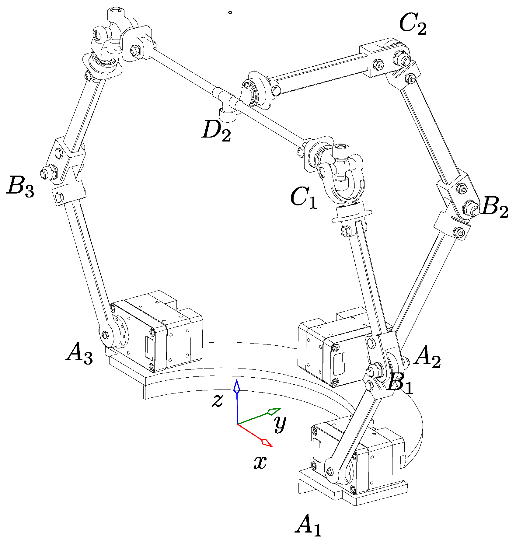
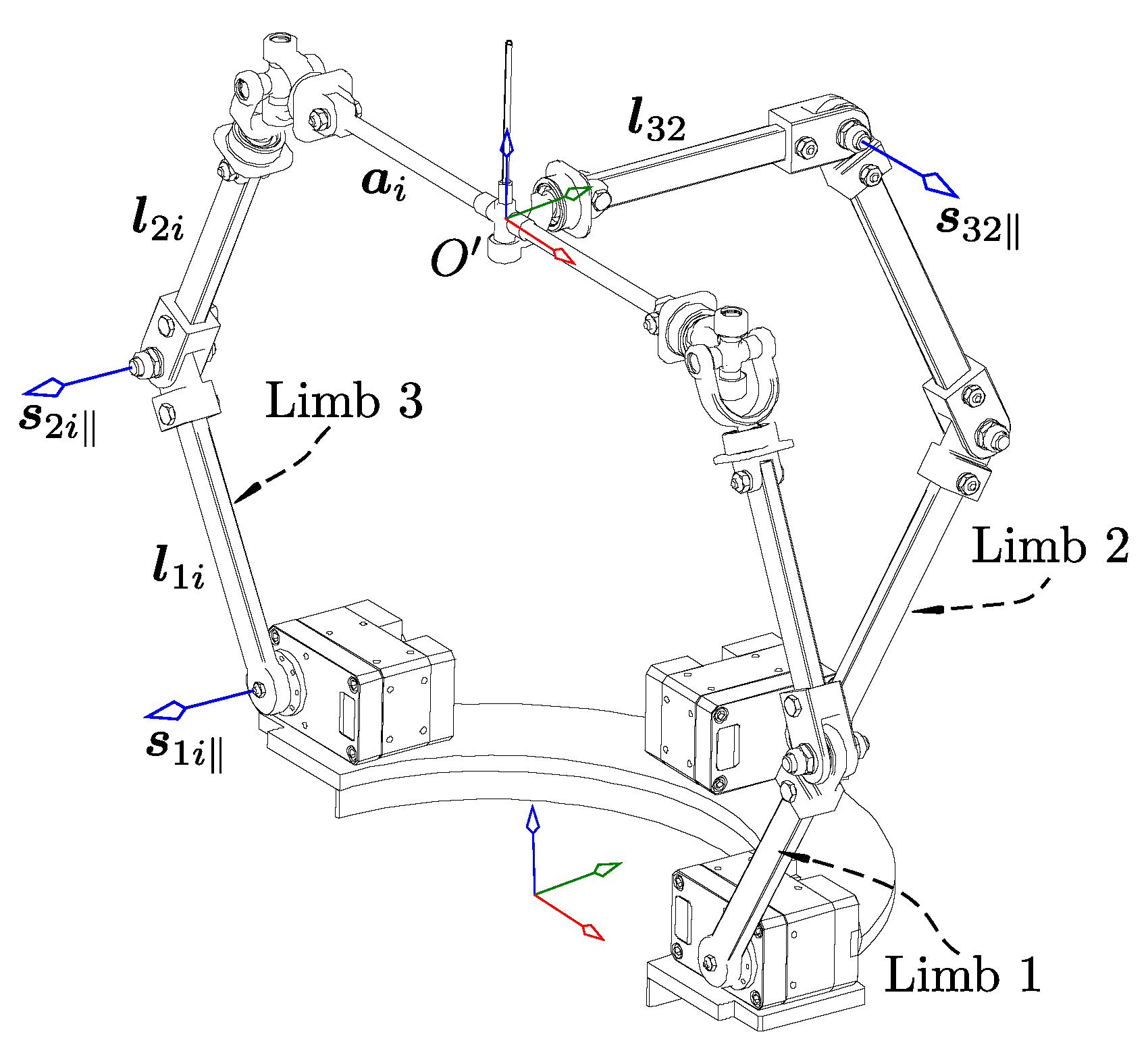
3. Kinematic Architecture of the Robot and Position Information

The conventional (rigid link-based) mechanism shown in Figure 3 should be described first for the purpose of kinematic analysis. The robot presented in this paper has partially decoupled three degrees of freedom (DoFs) motions contributed by the three limbs. The joints in the first and third limbs shown in Figure 3 are arranged in a revolute–revolute–spherical (RRS) sequence from base to top, and the first and third limbs are symmetrically aligned. The second limb’s spherical joint is decoupled to satisfy the condition to remove a parasitic motion [17,18]. Therefore, the joints in this limb are arranged in a revolute–revolute–universal (RRRU) order. Moreover, all actuators are located at the base; thus, each limb’s active joint is the first revolute joint. All direction and position vectors are represented in a fixed frame O. The robot’s lower links ( l 1 i = l 1 ) are identical and similarly, so are the upper links ( l 2 i = l 2 ). The origin of the moving frame on the moving plate is represented by O . All revolute joints in each limb are designed to be parallel and are represented by the direction vector s j i where j and i indicate the joint and corresponding limb numbers, respectively. The x-axis of the fixed frame is along the first limb. Limbs two and three are offset from the x-axis by ξ 2 = 90 and ξ 3 = 180 , respectively. The first limb is located on the x-axis of frame O and is ξ 1 = 0 . The radii of fixed and moving plates are represented by the constants r a and r b , respectively. The Lie group-based synthesis of the robot is presented in Appendix C while the list of symbols and abbreviations are provided in Appendix D. The vector b i describes the servo actuator’s center position from O, whereas a i is the position vector on the moving plate based on a fixed frame. These vectors are mathematically represented as
b i = R z ( ξ i ) T x ( r b )
a i = R a i , where a i = R z ( ξ i ) T x ( r p ) .
Note that the vector from O to the universal joint of the second limb is zero. Hence, the expression of a 2 = R a 2 = 0 .
The rotation matrix ( R ) describing the orientation of the moving plate with respect to the fixed frame is
R = R z ( ϕ ) R y ( θ ) R x ( ψ )
where ϕ is zero for this robot since there is no parasitic motion in its workspace.
The position of the first and second passive revolute joints and joints on the moving plate can be described by the following position vectors:
r 1 i = R z ( ξ i ) T x ( r b ) + R y ( θ 1 i ) T x ( l 1 )
r 2 i = R z ( ξ i ) ( T x ( r b ) + R y ( θ 1 i ) ( T x ( l 1 ) + R y ( θ 2 i ) T x ( l 2 ) )
Given g = R z ( ξ i ) 1 r 2 i T x ( r b ) , the active joint angle is obtained as
c θ 1 i s θ 1 i = c 1 z c 1 x c 1 z c 1 x 1 g x g z
Then, the passive joints value is solved as
c θ 2 i s θ 2 i = ( c 1 x l 1 ) / l 2 c 1 z / l 2
where c 1 x = ( g x 2 + g z 2 + l 1 2 l 2 2 ) / 2 l 1 and c 1 z = g x 2 + g z 2 c 1 x 2 . Finally, the last passive revolute joint of the second limb can be obtained as follows:
l 32 = R y ( θ ) R x ( ψ ) R z ( q z ) R y ( q y ) 0 r a 0 = 0 × ×
with an assumption that q y = θ , Equation (8) can be rewritten as
r a ( c θ s q z s θ s ψ c q z ) r a c ψ c q z r a s θ s q z = 0 × ×
Consequently, we obtain q z as in Equation (10)
q z = t 1 ( t θ s ψ )
where t denotes tan in Equation (10).
r 32 = r 22 + R z ( ξ 2 ) R y ( θ 12 ) R y ( θ 22 ) × R y ( θ 32 ) T x ( r a ) = ( r 21 + r 23 ) 2
Reorganizing and rewriting Equation (11) gives
R z ( ξ 2 ) R y ( θ 12 ) R y ( θ 22 ) R y ( θ 32 ) T x ( r a ) = ( r 21 + r 23 ) 2 r 22
Let d = ( r 21 + r 23 ) 2 r 22 and rearranging Equation (12), we get
R y ( θ 32 ) T x ( r a ) = [ R z ( ξ 2 ) R y ( θ 12 ) R y ( θ 22 ) ] 1 d
r a c θ 32 0 r a s θ 32 = d ¯ c θ 32 s θ 32 = d ¯ x r a d ¯ z r a .
Finally, the third angle of the second leg is obtained as
θ 32 = t a n 1 d ¯ z d ¯ x
Thus far, all the active and passive joints below the moving plate are known at the position level.

3.1. Main Kinematic Features of the Robot

3.1.1. Non-Parasitic Motion

The robot presented in this paper has been optimized to eliminate parasitic motion and does not exhibit any parasitic motion within its workspace. The three limbs are designed and configured in a way that completely removes the parasitic motion from the workspace, as illustrated in Figure 3. Detailed explanations of how this configuration achieves the elimination of parasitic motion are discussed in the authors’ recent work [17]. It is well-known that removing parasitic motion enhances accuracy, controllability, and enables safe interaction with the environment [10,12,17].

3.1.2. Simple to Manufacture and Control

One of the most vital features of the robot is its architectural simplicity. A robot with a simple architecture is easier to address in design, manufacture, assemble, and control. Although making a symmetric lower-DoF robot without parasitic motion presents challenges, we maintained its symmetric properties and common kinematic joints, which are essential for simplifying the architecture. Consequently, the designed robot features identical joints in the limbs and almost symmetric limbs, which helps avoid complex geometry while still removing parasitic motion and preserving other important features.

3.1.3. Compactness

In many instances, lower-DoF PRs are designed with linear actuators, as evidenced in various studies [9,10,12,14]. The preference for linear actuators stems from their ability to simplify mathematical models significantly. However, these robots demand a larger deployment area compared to those with rotational actuators. Rotational actuators offer the advantage of folding the robot, thereby reducing its volume, particularly when not in use. Additionally, linear actuators necessitate converting direct motor output into linear motion, which can be more complex. In contrast, using rotational actuators directly leads to a robot with a longer maintenance life, fewer components, and greater compactness. Given these considerations, the robot designed in this paper exclusively employs rotational servo actuators.

3.1.4. Partially Decoupled Motion

Leveraging the geometric conditions that facilitate the removal of parasitic motion, each limb can independently control one of the two rotational DoFs of the moving platform. Specifically, limb two is dedicated to generating rotation along the x-axis, while limbs one and three collaborate to produce motion along the y-axis. This design greatly simplifies control and enhances safety during the use of the robot.

3.1.5. Mechanically Constrained Pivoted Motion

Many lower-DoF PRs lack a fixed point on their moving plate relative to the fixed frame, a feature that is crucial in certain applications, such as medical robots. Although some previously developed spatial robots meet this requirement, they do not maintain it throughout the entire orientation workspace. A robot is considered to have pivot motion across its entire workspace if it can maintain a target point in a fixed position relative to the fixed frame while varying its orientation. The robot presented in this paper is designed to ensure that the position of the moving frame aligns with the z-axis during changes in orientation angles, achieved mechanically. This approach is safer than relying on a software-controlled pivot point type. This feature is especially important for robots used in surgical and observational applications. For instance, a surgical robot without a pivot point would require a larger incision, contradicting the principles of minimally invasive surgery. In general, a device lacking a pivot point can lead to inaccuracies and, to some extent, cause damage in its operation. Therefore, incorporating this pivotal feature is vital when designing robots for such specific applications.

4. Rate Kinematics with the Restriction Space

The rate kinematics equation of the robot is obtained analytically based on the concept of restriction space, which was originally introduced in [20,21], and can be described in a more general form as in Equation (14). Accordingly, the detailed elements of active and constraint wrenches are obtained from 5 $ 0 –1 $ screws. The screw representation comprises a direction and moment vectors. It is represented as $ j i = s a j i s a j i where s a j i and s a j i are the direction and moment vectors, respectively. Indices j and i indicate that the screw or a vector belong to the j t h joint in the i t h limb.
q ˙ a 0 = G a T G c T x ˙
Before solving the constraint and motion wrench of the limbs, the following vector relations need to be defined, where
l 5 i = l 1 i + l 2 i + l 3 i l 4 i = l 2 i + l 3 i l 2 i = r 2 i r 1 i l 1 i = r 1 i b i b i = R z ( ξ i ) T ( r b )
where l 31 = a 1 , l 33 = a 3 , l 32 a 2 , which is given by
l 32 = R y ( θ ) R x ( ψ ) R z ( q z ) R y ( q y ) T y ( r a )
The first and third limbs have an identical screw system where the temporary end-effector is assigned to be the center of spherical joints and then the constraint equation is obtained as
Limb   1   and   3 : s 5 i T 0 T s 4 i T 0 T s 3 i T 0 T s 2 i T ( s 2 i × l 2 i ) T s 1 i T ( s 1 i × l 3 i ) T s r i s r i = 0
where s r i and s r i are the restriction screw direction and moment vectors. The moment vector ( s r i ) can be derived as in Equation (16).
s r i = [ s 5 i · ( s 4 i × s 3 i ) ] ( r 52 × s 2 i ) × ( r 51 × s 1 i ) + [ s 5 i · ( s 3 i × s 1 i ) ] ( r 54 × s 4 i ) × ( r 52 × s 2 i ) [ s 5 i · ( s 4 i × s 1 i ) ] ( r 53 × s 3 i ) × ( r 52 × s 2 i ) + [ s 5 i · ( s 3 i × s 2 i ) ] ( r 54 × s 4 i ) × ( r 51 × s 1 i ) + [ s 5 i · ( s 4 i × s 5 i ) ] ( r 54 × s 4 i ) × ( r 53 × s 3 i ) + [ s 5 i · ( s 4 i × s 2 i ) ] ( r 53 × s 3 i ) × ( r 51 × s 1 i ) = s 1 i
Note that r 5 j = r 5 r j is the position vector between the first-row screw and the rest of the screws associated with the j t h joint. Since s 3 i , s 4 i , and s 5 i are located at the same position on the limb, r 54 = r 53 = 0 for the first and third limbs. Solving Equation (15) for the moment vector proves that s r i is always zero.
The second limb’s spherical joint is decoupled and it causes a different moment vector for $ 42 and $ 52 . Thus, the constraint equation to get this particular limb restriction is given by
Limb 2 : s 52 T ( 0 ) T s 42 T ( 0 ) T s 32 T ( s 32 × l 32 ) T s 22 T ( s 22 × l 42 ) T s 12 T ( s 12 × l 52 ) T s r 2 s r 2 = 0
Solving Equations (15) and (17) tells us that all limbs are restricted from the linear motion along the direction of the revolute joint axes, as in Equation (16). Then, the restriction information is embedded into the limb matrix to get the extended Jacobian.
J e i = J a i J c i
where J c i = 0 T s 1 i T T .
By removing the active joint screw from Equation (18) and nullifying the remaining set of screws, the active joint wrench for the first and third limb is obtained from the following constraint equation:
s 5 i T 0 T s 4 i T 0 T s 3 i T 0 T s 2 i T ( s 2 i × l 2 i ) T 0 T s 1 i T s a i s a i = 0 ,
s a i = [ s 5 i · ( s 3 i × s 2 i ) ] ( r 54 × s 4 i ) × s 1 i + [ s 5 i · ( s 4 i × s 2 i ) ] ( r 53 × s 3 i ) × s 1 i [ s 5 i · ( s 4 i × s 3 i ) ] ( r 52 × s 2 i ) × s 1 i
Solving Equation (19) and simplifying the result in Equation (20) gives the direction vector, s a i , which is the same as l 2 i and the detailed derivation of the moment vector can be found in Appendix B. The constraint screw is known by taking the elliptic polar [23] of the restriction screw.
Moreover, in the three limbs, we have four passive joints that are below the moving plate. Thus, by locking these joints sequentially, the corresponding wrench screws are obtained as shown below:
w p = ( l 11 + l 21 ) T ( ( l 11 + l 21 ) × a 1 ) T ( l 12 + l 22 ) T ( k 1 ( s 42 + s 52 ) ) l 12 T ( k 2 ( s 42 + s 52 ) ) ( l 13 + l 23 ) T ( ( l 13 + l 23 ) × a 3 ) T
where k 1 = s 32 T ( l 12 + l 12 ) × l 32 s 32 T ( s 42 × s 52 ) and k 2 = s 22 T l 12 × l 42 s 32 T ( s 42 × s 52 ) .
So far, all relations of limb 1 and limb 3 are derived for the isolated branch. In order to move the reference point to the center of the moving plate, the following screw transformation matrix is used:
M = I 0 [ a i ] × I
As a result, the active joint and constraint wrenches are pre-multiplying with the transformation matrix given in Equation (22) and the robot-level relation is known as shown in Equation (23), Equation (24), respectively.
w a = l 21 T ( l 21 × a 1 ) T l 22 T ( l 22 × ( s 32 · l 22 × l 32 s 32 · s 42 × s 52 s 42 × s 52 ) ) T l 23 T ( l 23 × a 3 ) T
w c = s 11 T ( s 11 × a 1 ) T s 22 T ( s 22 × 0 ) T s 31 T ( s 31 × a 3 ) T
Finally, the inverse Jacobian mapping all the active and passive joints’ velocity to the task-space motion is obtained as
q ˙ a q ˙ p 0 = q ˙ a q ˙ p 0 = G a T G p T G c T v ω
where
G a = l 21 T l 21 T ( s 11 × l 31 ) ( l 21 × a 1 ) T l 21 T ( s 11 × l 31 ) l 22 T l 22 T ( s 12 × l 52 ) + m 1 l 22 × s 32 · l 22 × l 32 s 32 · s 42 × s 52 s 42 × s 52 T l 22 T ( s 12 × l 52 ) + m 1 l 23 T l 23 T ( s 13 × l 33 ) ( l 23 × a 3 ) T l 23 T ( s 13 × l 33 )
G p = l 31 T l 31 T ( s 21 × l 21 ) T ( l 31 × a 1 ) T l 31 T ( s 21 × l 21 ) l 32 T k 1 ( s 42 × s 52 ) s 22 k 1 ( s 42 × s 52 ) k 1 ( s 42 × s 52 ) s 22 l 33 T l 33 T ( s 23 × l 23 ) T ( l 33 × a 3 ) T l 33 T ( s 23 × l 23 )
G c = s 11 T ( s 11 × a 1 ) T s 12 T 0 T s 13 T ( s 13 × a 3 ) T v ω
and m 1 = l 22 × s 32 · l 22 × l 32 s 32 · s 42 × s 52 s 42 × s 52 T s 12 .
From the inverse-rate kinematic equation given in Equation (14), the task velocity ( x ˙ ) has to be known. In the usual type of lower-DoF robots, x ˙ cannot be given arbitrarily since it is required to satisfy the structural constraint G c T x ˙ = 0 . However, this robot is parasitic motion-free and only three independent terms should exist in the task space. Thus, we do not need an extra step to derive the expression relating parasitic and independent terms. This can be proven by the filtering matrix and velocity level coupling relation shown in Equation (26), Equation (27) where the details can be found in [11,18].
x ˙ = ( I G c G c ) x ˙ a
v x v y ω z = C 1 1 C 2 ω x ω y
where
C 1 = s ξ 1 c ξ 1 ( a 1 x c ξ 1 + a 1 y s ξ 1 ) s ξ 2 c ξ 2 ( a 2 x c ξ 2 + a 2 y s ξ 2 ) s ξ 3 c ξ 3 ( a 3 x c ξ 3 + a 3 y s ξ 3 ) and
C 2 = a 1 z c ξ 1 a 1 z s ξ 1 a 2 z c ξ 2 a 2 z s ξ 2 a 3 z c ξ 3 a 3 z s ξ 3 .
In Equation (27), we got the parasitic motion governing equation, which will be used for the cost function during optimization.

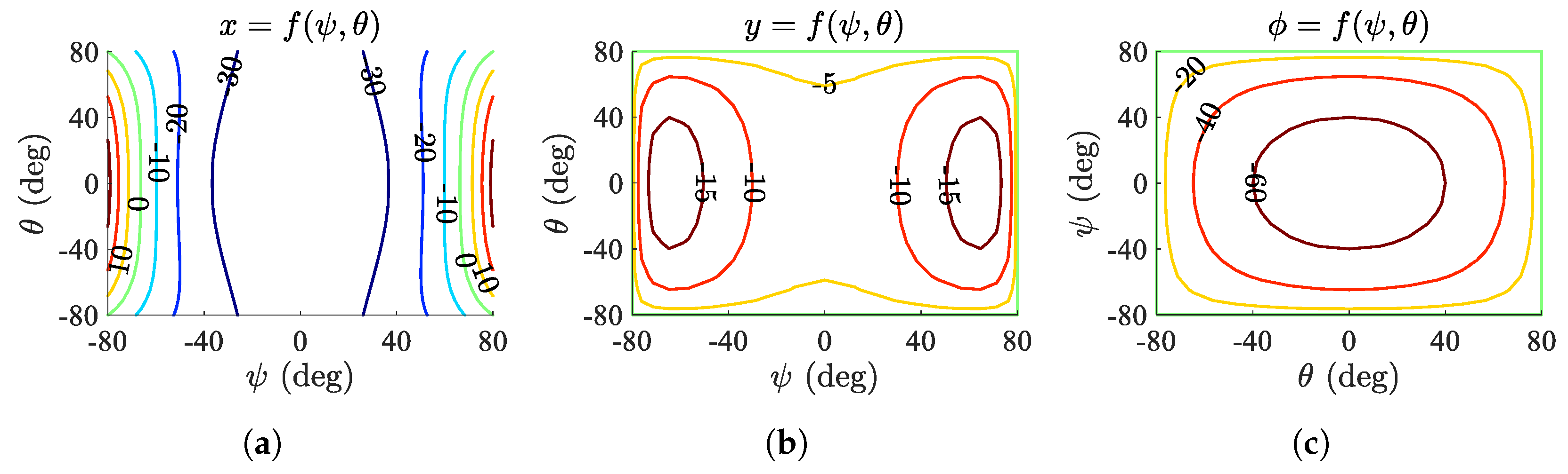
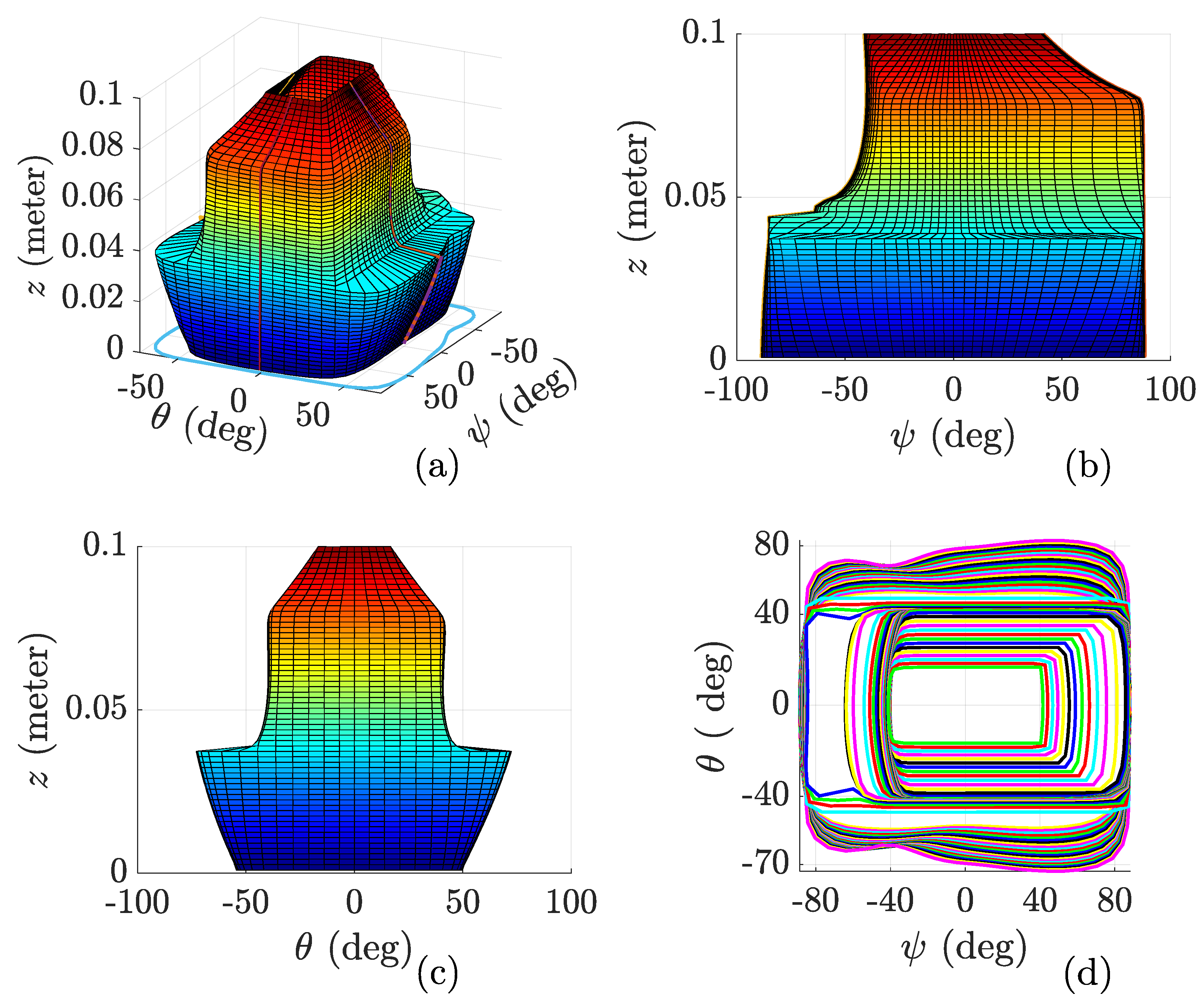
5. Optimization of Parasitic Motion

Once the coupling relation shown in Equation (27) is obtained, it can be used to formulate the optimization cost function. First, let
C 1 = x 0 x 1 x 2
where each x i R 3 is a column vector.
Then, let the determinant of C 1 be
det ( C 1 ) = x 0 · x 1 × x 2
where x 0 , x 1 , and x 2 denote the columns of C 1 . The inverse of C 1 is thus
C 1 1 = 1 det ( C 1 ) ( x 1 × x 2 ) ( x 2 × x 0 ) ( x 0 × x 1 )
Consequently, for a given input ω = [ ω x , ω y ] , the parasitic motion vector is analytically given by
v x v y ω z = 1 x 0 · x 1 × x 2 ( x 1 × x 2 ) ( x 2 × x 0 ) ( x 0 × x 1 ) a 1 z c ξ 1 a 1 z s ξ 1 a 2 z c ξ 2 a 2 z s ξ 2 a 3 z c ξ 3 a 3 z s ξ 3 ω x ω y
where each term is an explicit function of the design parameters { ξ i , a i x , a i y , a i z } for i = 1 , 2 , 3 . Then, we obtain and explicit form of the parasitic components as
v x = ( x 1 × x 2 ) x 0 · ( x 1 × x 2 ) a 1 z c ξ 1 a 1 z s ξ 1 a 2 z c ξ 2 a 2 z s ξ 2 a 3 z c ξ 3 a 3 z s ξ 3 ω x ω y
v y = ( x 2 × x 0 ) x 0 · ( x 1 × x 2 ) a 1 z c ξ 1 a 1 z s ξ 1 a 2 z c ξ 2 a 2 z s ξ 2 a 3 z c ξ 3 a 3 z s ξ 3 ω x ω y
ω z = ( x 0 × x 1 ) x 0 · ( x 1 × x 2 ) a 1 z c ξ 1 a 1 z s ξ 1 a 2 z c ξ 2 a 2 z s ξ 2 a 3 z c ξ 3 a 3 z s ξ 3 ω x ω y

5.1. Cost Function Formulation

The above equation is thus formulated as a multi-objective optimization problem as
min ξ , a z F ( ξ , a z ) = | v x ( ξ , a z ) | | v y ( ξ , a z ) | | ω z ( ξ , a z ) |
subject to
ξ X , a z A
where X and A denote the feasible design parameter sets. In fact vector a z can be further expanded from R R z ( ξ ) T x ( r p ) , which gives us a i z = r 31 r p c ξ i + r 32 s ξ i . This reveals that the specific variables that affect the parasitic motion are r p , ξ 1 , ξ 2 , and ξ 3 . Here, the rotation matrix given in Equation (3) is rewritten as R = r 11 r 12 r 13 r 21 r 22 r 23 r 31 r 32 r 33 .
Thus, a solution ( ξ i * , r z * ) is Pareto-optimal if there does not exist another feasible solution ( ξ , r p ) such that
F ( ξ , r p ) F ( ξ * , r p * ) and F ( ξ , r p ) F ( ξ * , r p * )
where the inequality is understood component-wise. To solve Equation (35), a particle swarm-based multi-objective optimization algorithm is employed to efficiently approximate the Pareto front of non-dominated solutions, thus providing a diverse set of optimal trade-offs among the objectives. For increased design flexibility, the radius of the moving platform, r p , is treated as a vector of independent variables, i.e., r p = r p 1 r p 2 r p 3 T , allowing each limb to have a distinct attachment radius.
According to the results of the optimization, setting r p 3 to a very small value or zero, and choosing ξ 1 = 0 , ξ 2 = 90 , and ξ 3 = 180 can completely eliminate parasitic motion from the workspace. However, a configuration with r p 3 = 0 is not practically feasible. To address this, the third limb’s spherical joint can be replaced by a combination of revolute and universal joints, with an offset link l 32 inserted between them. This modification enables the realization of a functionally parasitic motion-free robot, as proposed in this work.

5.2. Comparison with Previous Robots

The robot presented in this paper is capable of a large orientation angle variation range, which is the most important feature but always challenging to achieve in PRs. For example, Yasir et al.’s [13] robot has ψ = ± 15 and θ = ± 20 , which is smaller than the orientation capability of the proposed robot. Although Kuo et al. [2] have claimed their design is able to achieve ± 60 , its kinematic architecture is extremely complex and thus, it could be difficult to manufacture or accurately transmit the input motion to the surgical tool. Moreover, the proposed robot has a partially decoupled DoF and thus, it is identical to [13] in this regard. Table 1 describes the kinematic features of the proposed robot along with existing robots designed for similar purposes.
The repeatability of the robotic systems was measured by repeatedly commanding the end-effector to return to a specific pose and recording its position using a 2D laser displacement sensor ((Keyence IL Series, Keyence Corp., Osaka, Japan) with sub-0.02 mm precision. The sensor was mounted on a rigid frame and aligned to target a fixed point on the end-effector along the z-axis. The standard deviation of these measurements over 20 cycles was calculated, resulting in the reported repeatability value of 0.05 mm in Table 1.

6. Design, Manufacturing, and Control

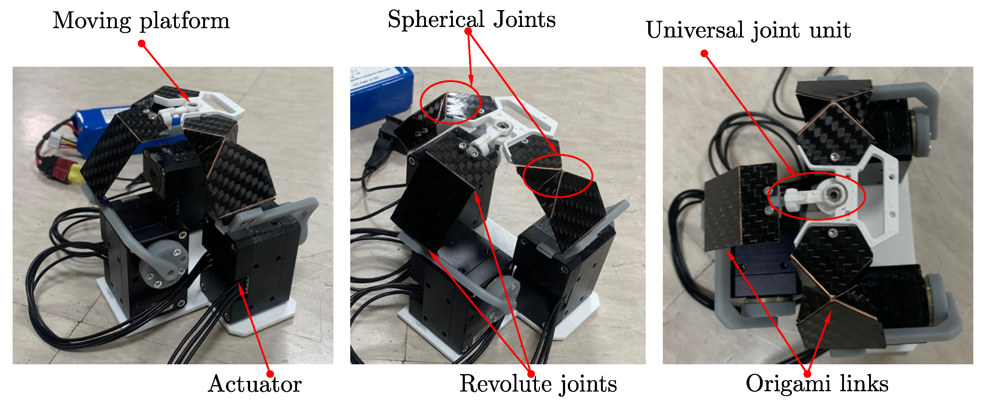
6.1. Design and Manufacturing

The proposed robot, whose 3D model is shown in Figure 4, is designed with scalability, ease of manufacturing, and straightforward control in mind, while also allowing for the simple replacement of failed components. A key aspect of the design philosophy is the structural uniformity of the limbs; all limbs are made as identical as possible to streamline fabrication and assembly. The links connecting the actuators to the end-effector can be realized using either conventional jointed linkages or origami-inspired folded carbon plate structures. In both configurations, three rotational servomotors located at the base actuate the limbs to generate the desired end-effector motion.

6.2. Hardware Design and Implementation

A personal computer acts as the central control unit of the system, communicating with three Dynamixel XL430-W250-T servomotors (Robotis, Seoul, Republic of Korea) via the U2D2 interface. Each servo is addressed using a unique ID, and receives specific target angles computed by the control software. The U2D2 interface not only transmits commands but also facilitates real-time feedback by relaying servo status data—such as position and velocity—back to the PC over a serial communication channel. The control software includes an inverse-rate kinematics solver that computes the required servo angles based on the desired end-effector position and orientation. This allows real-time execution of target trajectories with high precision.

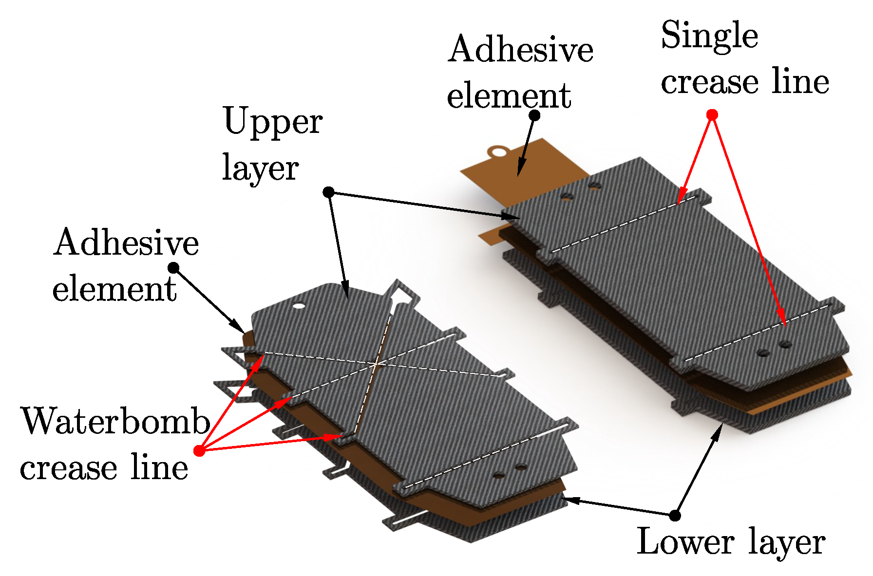
Transformation to an Origami-Based Parallel Robot

Integrating origami-inspired design principles into the robot architecture introduces several advantages, including a reduction in the number of components, simplified assembly, flat-foldability, and enhanced scalability. In this transformation, depicted in Figure 5, conventional links and joints are reinterpreted as crease lines and vertices within the origami paradigm. Specifically, a single-crease folding line between adjacent rigid plates functions analogously to a revolute joint. The spherical joint is replaced by a single-vertex, six-crease configuration known as a waterbomb base [24].
To eliminate parasitic motion, the spherical joint in the second limb is replaced by a revolute–universal joint pair, as suggested in previous literature [9,17]. However, due to the lack of a suitable origami equivalent for a universal joint, a hybrid approach is adopted: the universal joint is realized using a compact linkage-based design and integrated at the distal end of the second limb.
The transformation process—from conventional joint-based linkage to an origami-style structure—is illustrated in Figure 5. Each origami limb is fabricated by bonding two carbon plates using a strong adhesive layer. After assembly, high pressure is applied to ensure proper adhesion, and the edges of the plates are trimmed using a precision cutter to enable the free movement required for revolute and spherical joint functionality. The linkage-based universal joint is fabricated separately and mechanically interfaced with the origami structure of the second limb.
Figure 6 displays the actual implementation of the robot, demonstrating the physical realization of the CAD design integration of origami-inspired components and actuators.

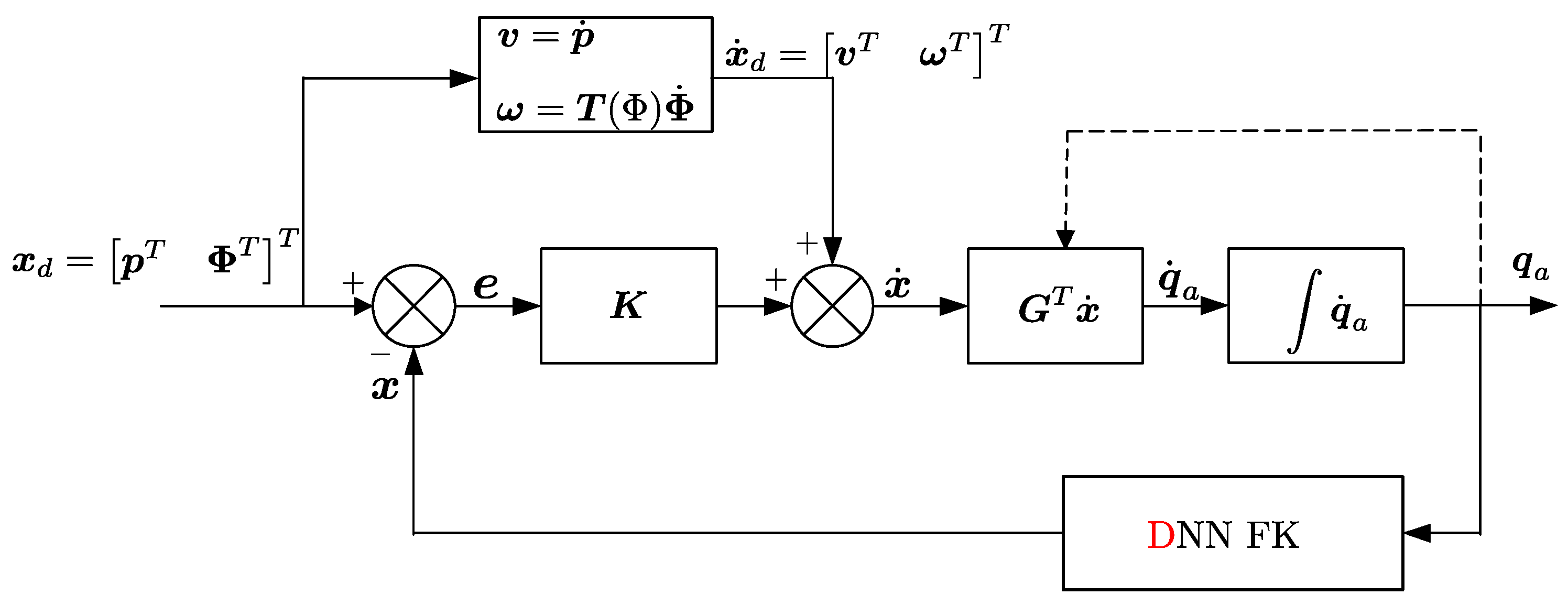
6.3. DNN-Blended Control Scheme

Building on the closed-form kinematic analysis in Section 4, we devise a hybrid control law that embeds a DNN-based forward-kinematics estimator within a classical velocity-feedback loop. This architecture unifies
  • Robust feedback: a Cartesian gain matrix K R 6 × 6 ensures asymptotic error convergence and disturbance rejection.
  • Adaptive compensation: a feedforward DNN approximates nonlinear FK under flexural and geometric uncertainties.
Let the desired pose trajectory be
x d ( t ) = p d ( t ) T Φ d ( t ) T T R 6 ,
with velocity
x ˙ d = p ˙ d T ω d T T , ω d = T ( Φ d ) Φ ˙ d .
At each control instant t k , the loop executes (see Algorithm 1). Figure 7 illustrates the block diagram: the DNN’s FK output closes the sensing loop without relying on symbolic inversion.
Algorithm 1 Hybrid DNN-blended control loop
Require: 
Desired trajectory { x d ( t k ) } , initial q a ( 0 ) , sampling Δ t
Ensure: 
Joint commands { q ˙ a ( t k ) }
1:
for  k = 0 to N 1  do
2:
     x ^ ( t k ) f θ ( q a ( t k ) )
3:
     e ( t k ) x d ( t k ) x ^ ( t k )
4:
     x ˙ ( t k ) K e ( t k )
5:
     q ˙ a ( t k ) G T ( q a ( t k ) ) x ˙ ( t k )
6:
     q a ( t k + 1 ) q a ( t k ) + q ˙ a ( t k ) Δ t
7:
end for
▹ DNN FK estimate

 
The DNN-blended control architecture illustrated in Figure 7 seamlessly integrates classical trajectory tracking control with deep neural network (DNN)-based state estimation to enhance overall system accuracy and robustness. In this approach, the desired Cartesian trajectory ( x d )—comprising both positional ( p ) and orientational ( Φ ) components—is first converted into corresponding velocity commands through a systematic velocity mapping. These commands, augmented by velocity feedback, are processed through the analytic Jacobian ( G T ) to obtain joint-space velocities ( q ˙ a ). Subsequently, these velocities are integrated to yield actuated joint angles ( q a ). Concurrently, the actual Cartesian pose ( x ) is estimated by a trained DNN forward kinematics (FK) model, providing real-time, accurate state feedback. This integration significantly improves trajectory tracking precision by mitigating errors arising from modeling uncertainties and external disturbances, which is particularly critical for high-precision applications.

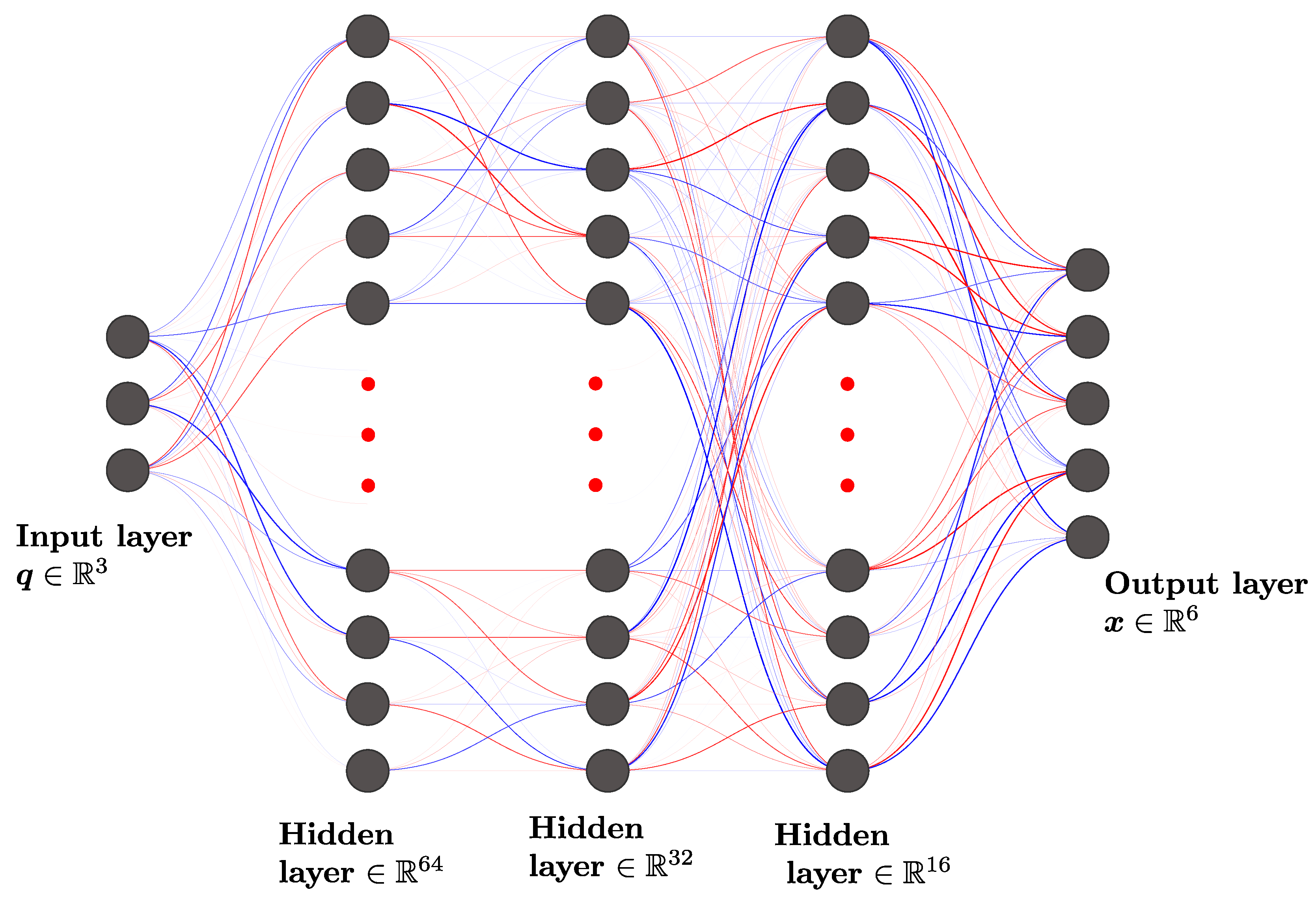
6.4. Deep Learning for State Estimation

To compensate for unmodeled flexure, backlash, and assembly tolerances, we trained a fully connected feedforward DNN to approximate
x ^ = f θ ( q a ) ,
where q a R 3 is the actuator-space input and x ^ R 6 the pose output.
Dataset generation and noise injection: The DNN was trained on a dataset of N = 50 , 000 joint–pose pairs, sampled uniformly across the robot’s workspace. To improve robustness and mimic realistic operating conditions, Gaussian noise was injected into the training data with standard deviations of 0.02 rad for joint angles, 0.1 mm for position, and 0.1 mrad for orientation. This approach enables the DNN to generalize reliably under sensor noise and modeling errors encountered in practice.

6.4.1. Network Architecture

Guided by universal approximation and empirical best practice, we adopt a “funnel” topology (3–64–32–16–6) as depicted in Figure 8:
3 Dense + ReLU 64 Dense + ReLU 32 Dense + ReLU 16 Linear 6 .
Mathematically,
h ( 1 ) = ReLU W ( 1 ) q a + b ( 1 ) , W ( 1 ) R 64 × 3 ,
h ( 2 ) = ReLU W ( 2 ) h ( 1 ) + b ( 2 ) , W ( 2 ) R 32 × 64 ,
h ( 3 ) = ReLU W ( 3 ) h ( 2 ) + b ( 3 ) , W ( 3 ) R 16 × 32 ,
x ^ = W ( 4 ) h ( 3 ) + b ( 4 ) , W ( 4 ) R 6 × 16 .
This layered reduction balances expressive capacity (64 neurons) with generalization (16-neuron bottleneck), facilitating rapid training and low inference latency.

6.4.2. Offline Training Algorithm

We trained on D = { ( q a ( i ) , x ( i ) ) } i = 1 N via mini-batch gradient descent (Algorithm 2).
The algorithmic complexity is as follows: forward pass O ( 3 · 64 + 64 · 32 + 32 · 16 + 16 · 6 ) = O ( 4608 ) FLOPs, backward pass 2 × . By integrating Algorithms 1 and 2, the DNN-blended controller attains both stability (via classical feedback) and high fidelity in the presence of real-world uncertainties.
Algorithm 2 Offline DNN training procedure
Require: 
Dataset D , epochs E, batch size B, learning rate α , weight decay λ
Ensure: 
Trained parameters θ
1:
Initialize θ with He initialization
2:
for epoch = 1 to E do
3:
    Shuffle D
4:
    for each mini-batch B D  do
5:
        Compute gradient θ L B ( θ ) + λ θ
6:
         θ θ α θ L B ( θ )
7:
    end for
8:
end for

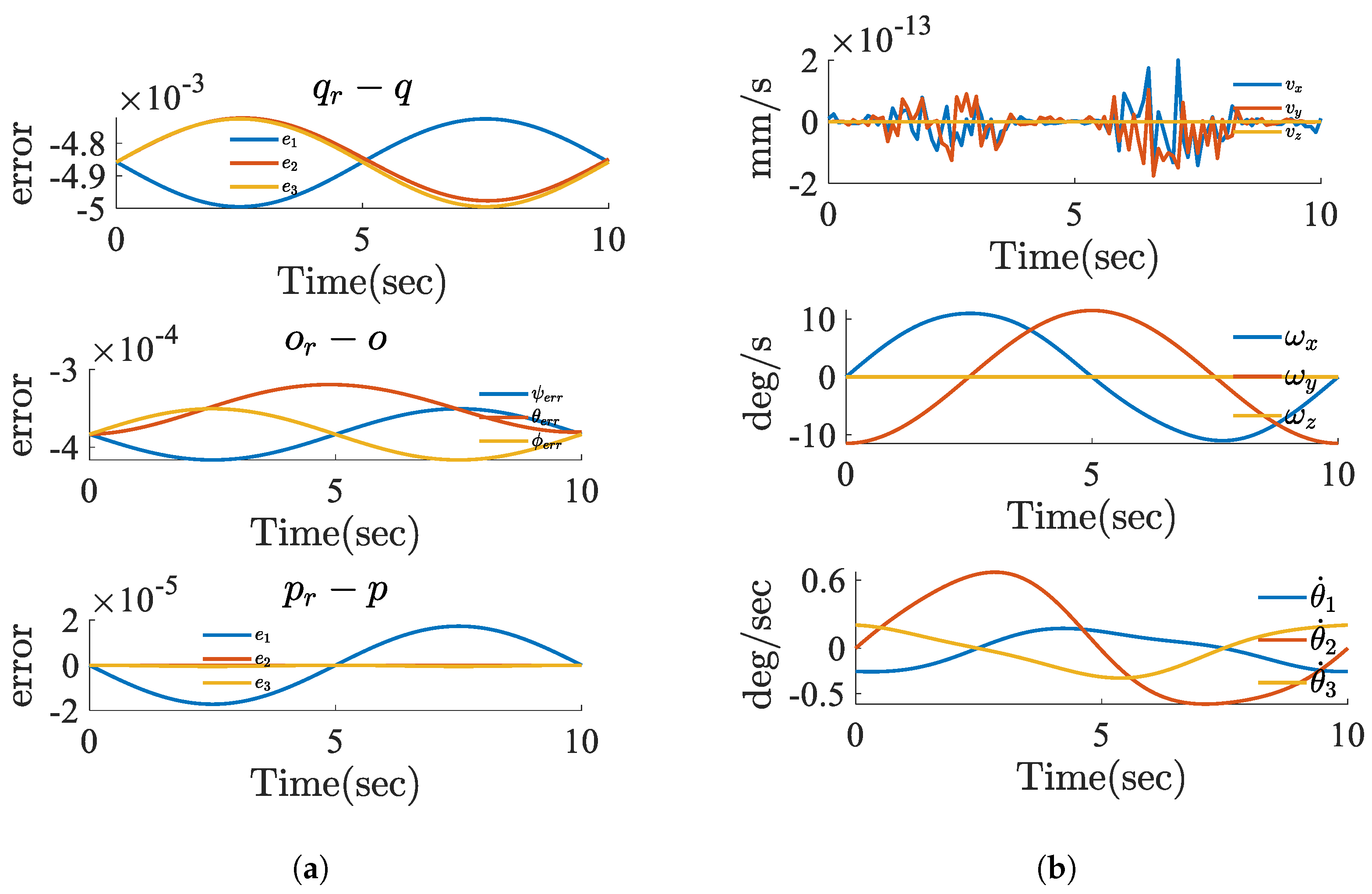
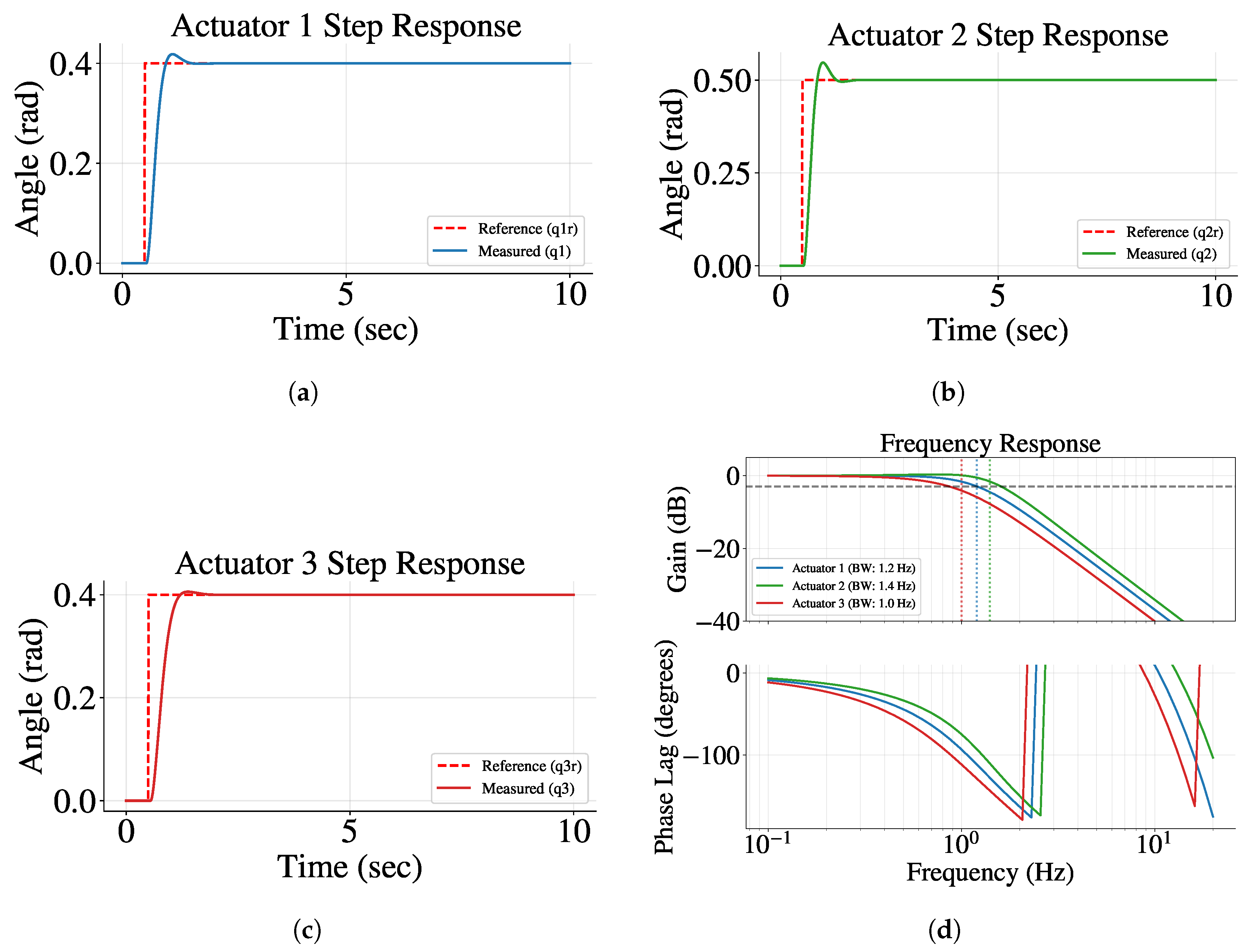
7. Simulation and Experimental Results

The following geometric parameters were used to generate the numerical simulation of the joint motion and workspace. These parameters were r b = 45 mm, l 1 i = 90 mm, l 2 i = 76.5 mm, l 32 = 68 mm, and r a = 135 mm.
Figure 9a presents a detailed comparison between the actual and reference pose of the moving platform, the reference is user input while the actual is predicted via DNN.
Figure 9b presents a detailed comparison between the actual and reference joint angles, emphasizing the high precision and effectiveness of the controller in minimizing joint angle tracking errors across all three actuators.
Figure 10a presents the error metrics in both joint space and task space, including joint angle, position, and orientation discrepancies, each computed as the difference between the reference trajectory and the actual measured values. The results confirm that the controller achieves high tracking accuracy, with joint, position, and orientation errors remaining within very small bounds throughout the operation. Figure 10b shows the task-space and joint-space velocity profiles obtained from the inverse-rate kinematics (IRK) formulation. The top row illustrates that the linear task-space velocities ( v x , v y , v z ) are effectively zero, indicating the absence of unintended parasitic motion during the intended motion. The angular task-space velocities ( ω x , ω y , ω z ) and the resulting joint velocities ( θ ˙ 1 , θ ˙ 2 , θ ˙ 3 ) closely match the theoretical predictions, validating both the controller performance and the accuracy of the IRK computation. These results are fully consistent with the expected theoretical behavior described in Equation (26).
The unit step and frequency response evaluation shown in Figure 11a–d of the actuators in a robot’s heave motion (z-axis translation) configuration demonstrates consistent and robust performance, where all three actuators are driven in synchrony. Step response tests reveal fast rise times (0.25–0.35 s), short settling times (1.0–1.5 s), and minimal overshoot (<8%), with all actuators closely tracking the reference trajectory (RMS error < 0.05 rad) and exhibiting a maximum inter-actuator delay of only 60 ms. Frequency-domain analysis confirms an operational bandwidth of 1.0–1.4 Hz for all actuators, ensuring accurate and stable tracking of low-frequency trajectories (<1 Hz) commonly encountered in precise pick-and-place or assembly tasks. Beyond this range, gain and phase roll-off characteristics are typical of well-tuned servo systems. The results further highlight the need for predictive or feedforward elements to compensate for transport delays and for resonance mitigation strategies in higher-speed scenarios. Overall, the actuators provide reliable, coordinated control for accurate z-axis translation within the robot’s typical operational envelope.
Figure 12 illustrates the robot’s workspace and its boundary projected onto the ψ θ plane, clearly indicating the extensive rotational capabilities of the robot about the x- and y-axes, thus validating its suitability for applications requiring significant orientational flexibility. The workspace is computed by evaluating the Jacobian determinant across the full range of actuated variables. To ensure all included points are free from Type 2 (first-order) singularities, only configurations satisfying | det ( G ) | > 10 6 were retained. This threshold, commonly used in computational kinematics, accounts for numerical precision limits while conservatively excluding near-singular configurations to guarantee reliable and safe manipulator performance.
The errors computed as the differences between the reference and actual joint angles, platform position, and velocities validate the performance of the DNN-based controller. Specifically, the consistently low error magnitudes across all metrics confirm that the controller is capable of accurately tracking the desired trajectories. This demonstrates that the controller operates within the required precision and maintains reliable performance throughout the task execution.
To evaluate the durability of the waterbomb-based spherical and hybrid universal joints, fatigue tests revealed crack onset after about 200,000 cycles under a 500 g load at 20 Hz, confirming both high endurance and the need for further material improvement. Backlash is minimized by sandwiching a polyimide film between precision-cut carbon plates, ensuring stable crease-line geometry. Compliance is reduced through a non-stretchable adhesive polyimide layer embedded between fiberglass plates, enabling accurate rotational motion with negligible elastic deformation, thus requiring no control compensation.

8. Conclusions

This paper presents the design of a novel three-DoF robot with key kinematic features such as non-parasitic motion, pivoted orientation motion, partially decoupled DoFs, simple kinematic architecture, and compactness. The designed mechanism enables pivoted motion around the origin of the moving frame. First, the rate kinematics are described using restriction space and screw theory. Then, the constraint projection matrix is employed to map the user’s desired task velocity to the constraint-compatible motion of the robot. By expressing the dependent motion of the moving plate in terms of the independent ones, parasitic motion is proven to be null across the entire task space.
The robot’s workspace is plotted and compared with other similar existing mechanisms. The DNN-based controller is validated by comparing the reference and actual angles, positions, and velocities, confirming that it accurately tracks the desired trajectories with minimal error, demonstrating the controller’s high precision and reliability. The results show that the proposed robot’s performance is highly competitive, with some aspects outperforming existing mechanisms.
The miniaturized nature of the robot, combined with its high precision and robustness, makes it ideal for various applications requiring 1T2R motion. Notably, it satisfies the stringent requirements of medical devices, such as minimally invasive surgical robots, and can also be adapted for use in deep-space observatories and robotic machining devices, where only three DoFs are required.

Author Contributions

Conceptualization, methodology, software, validation, formal analysis, investigation, resources, data curation, and project administration, H.N.; writing—original draft preparation, writing—review and editing, and funding acquisition, G.S.; supervision, Z.W.; visualization, Y.H. All authors have read and agreed to the published version of the manuscript.

Funding

This research was funded by the Yuyao Robotics Research Center through the projects “Design and Control of the Dual Arms of Humanoid Robots” (Grant No. KZ22305) and “Robotic VR Controller” (Grant No. KZ22308); by the project “Design and Fabrication of an Immersive Interactive VR Robot Controller” under the Ningbo Yongjiang Talent Program (Grant No. Z22501); and by the Zhejiang Talents Program.

Data Availability Statement

Data are contained within the article.

Conflicts of Interest

The authors declare no conflicts of interest.

Appendix A. Solution to the Composite Joint Angles

H = H 1 H 2 H 3 H 4 H 5 H 6 = R R T x ( r a ) + p 0 1
where
H 1 = I T x ( r b ) 0 1 H 2 = R y ( θ 1 i ) R y ( θ 1 i ) T x ( l 1 i ) 0 1 H 3 = R y ( θ 2 i ) R y ( θ 2 i ) T x ( l 2 i ) 0 1 H 4 = R y ( θ 3 i ) 0 0 1 H 5 = R x ( θ 4 i ) 0 0 1 H 6 = R z ( θ 5 i ) 0 0 1
Equating only the rotational part of Equation (A1), gives the solution to all spherical joint angles for i = 1 , 3 .
For the universal joint angle associated with the second limb, there are only two passive joint angles. Since the joint is located at the origin of the moving frame, its motion is the same as that of the moving plate. Hence,
Q = Q 1 Q 2 Q 3 Q 4 Q 5 Q 6 Q 7 Q 8 Q 9 Q 10 = R p 0 1
where
Q 1 = R z ( ξ 2 ) 0 0 1 Q 2 = I T x ( r b ) 0 1 Q 3 = R y ( θ 12 ) 0 0 1 Q 4 = I T x ( l 12 ) 0 1 Q 5 = R y ( θ 22 ) 0 0 1 Q 6 = I T x ( l 22 ) 0 1 Q 7 = R y ( θ 32 ) 0 0 1 Q 8 = I T x ( l 32 ) 0 1 Q 9 = R x ( θ 42 ) 0 0 1 Q 10 = R z ( θ 52 ) 0 0 1

Appendix B. Derivation of the Actuated Joint Wrench Moment Vector

In Section 4, the direction vector of the active joint wrench was identified. Therefore, the detailed derivation of the moment vector is presented in this section. By using the constraint equation shown in Equation (17), limb 2 can be expressed as follows:
s 52 T 0 T s 42 T 0 T s 22 T ( s 22 × l 42 ) T s 12 T ( s 12 × l 52 ) T 0 T s 12 T s a 2 s a 2 = 0 ,
The direction vector s a 2 is identified and is equal to vector l 22 as described in Equation (23).
The moment vector s a 2 must satisfy
s 52 T s a 2 = 0
s 42 T s a 2 = 0
s 32 T s a 2 + ( s 32 × l 32 ) T s s a 2 = 0
s 12 T s a 2 + ( s 22 × l 42 ) T s a 2 = 0
s 12 T l 12 = 0
The relation in Equation (A8) is always zero because s 12 l 22 , where s a 2 = l 22 .
From Equations (A4) and (A5), s p 2 must be perpendicular to both s 52 and s 42 .
s p 2 = k ( s 52 × l 32 ) where k is a scalar for adjusting the vector .
From Equations (A6) and (A7),
s 32 T ( s a 2 + ( l 32 × s a 2 ) ) = 0
s 22 T ( s a 2 + ( l 42 × s a 2 ) ) = 0
and
s 32 T ( k ( s 52 × l 32 ) + ( l 32 × l 22 ) ) = 0
s 22 T ( k ( s 52 × l 32 ) + ( l 32 × l 22 ) ) = 0
Both s 22 and s 32 are parallel to ( l 32 × l 42 ) but not parallel to ( s 52 × s 42 ) .
l 32 and l 22 are on the yz plane and thus ( l 32 × l 22 ) is along the x-axis, i.e.,
l 32 × l 22 = l x 0 0
In order for Equations (A4) and (A5) (consequently Equations (A6) and (A7)) to be zero,
k ( s 52 × l 32 ) + ( l 32 × l 22 ) = k ( c θ s q z c q z s ψ s θ ) + l x k c ψ c q z k ( s q z s θ c q z c θ s ψ )
must be perpendicular to s 32 and s 22 . s 32 and s 22 are directed to the x-axis, i.e., s 32 = s 22 = [ 1 , 0 , 0 ] T . Then, the elements becomes
k ( c θ s q z c q z s ψ s θ ) + l x = 0
k = l x / ( c θ s q z c q z s ψ s θ ) )
Finally, the moment vector becomes
s a 2 = l x ( t q z t θ sin ψ ) ( c θ s q z c q z s ψ s θ ) k c ψ c q z k ( s q z s θ c q z c θ s ψ )
where s , c , and t stand for sin , cos , and tan, respectively.

Appendix C. Lie Group-Based Synthesis of the PR

Considering a serial kinematic chain, which consists of links and joints, the permissible relative displacements among the links are a subset of the Lie group of rigid body displacements [12,25]. Please refer to Figure 2, which illustrates the representations used in the following equations.
Figure A1. Manipulator schematics (3D).
Actuators 14 00291 g0a1
According to Lie group theory, the kinematic bond generated by each limb represents a five-dimensional (5D) displacement manifold, which is described as follows:
{ L 1 } = { R ( A 1 , y ) R ( B 1 , y ) S ( C 1 ) } { L 2 } = { R ( A 2 , x ) R ( B 2 , x ) R ( c 2 , x ) { R ( O , y ) } { R ( O , z ) } { L 3 } = { R ( A 3 , y ) R ( B 3 , y ) S ( C 2 ) }
where R ( point , axis ) represents the revolute joint located at the “ point ” while its rotation is parallel to the “ axis ”. The { S ( C i ) } represents the spherical joint motion located at point C i .
Applying the product closure in displacement [25,26], the intersection of { L 1 } and { L 3 } is obtained as
{ L 1 } { L 3 } = { G ( y ) } { S ( C 1 ) } { G ( y ) } { S ( C 2 ) } = { G ( y ) } { S ( C 1 ) } { S ( C 2 ) } = { G ( y ) } { R ( O , x ) }
Then, the platform displacement set is obtained by taking the intersection of all three limbs as
{ L 1 } { L 3 } { L 2 } = { G ( y ) } { R ( O , x ) } { G ( x ) } { R ( O , y ) } { R ( O , z ) } = { T ( y ) } { R ( O , y ) } { R ( O , x ) } { T ( x ) } { R ( O , x ) } { R ( O , y ) } { R ( O , z ) } = { R ( O , x ) } { R ( O , y ) } { T ( y ) } { T ( x ) } { R ( O , z ) } = { R ( O , x ) } { R ( O , y ) } { T ( z ) }
According to Equation (A20), the proposed robot has three-DoF motions and these are translational along z-axis and rotational about x ( y ) axes.

Appendix D. Nomenclature

Here, we provided the list of symbols, abbreviations, their physical meanings, and corresponding units.
Table A1. A complete list and definition of variables and abbreviations used.
SymbolDescription
Mathematical Symbols
ψ , θ , ϕ Orientation angles (Euler angles for roll, pitch, and yaw)
RRotation matrix of the moving platform
ξ i Angular offset of limb i from the x-axis (e.g., ξ 1 = 0 , ξ 2 = 90 )
l 1 Length of lower links (identical across limbs)
l 2 Length of upper links (identical across limbs)
r a Radius of the fixed base plate
r b Radius of the moving platform
OFixed reference frame
O Moving reference frame attached to the platform
s j i Direction vector of joint j in limb i
a i Position vector from O to joint center (spherical/universal)
b i Position vector from O to base actuator center
R x , R y , R z Rotation matrices about x , y , and z-axes
T x Translation matrix along the x-axis
q ˙ a Active joint velocity vector
x ˙ Task-space velocity twist ( [ v T ω T ] T )
G c , G e Constraint and motion wrench matrices
$ j i Screw representation of joint j in limb i ( [ s T s T ] T )
v x , v y , v z Linear velocity components
ω x , ω y , ω z Angular velocity components
ζ Design parameter vector ( ξ 1 , ξ 2 , ξ 3 )
det ( G ) Determinant of the Jacobian (singularity condition)
Abbreviations
DoFDegrees of Freedom
PRParallel Robot
DNNDeep Neural Network
IT2R/1T2ROne Translation + Two Rotational Motions
RRSRevolute–Revolute–Spherical Limb
RRRURevolute–Revolute–Revolute–Universal Limb
CNCComputer Numerical Control
CMMCoordinate Measuring Machine
VRVirtual Reality
MISMinimally Invasive Surgery
FKForward Kinematics
IRKInverse-Rate Kinematics
RRevolute Joint
PPrismatic Joint
SSpherical Joint
UUniversal Joint
BWBandwidth (Control Systems)

References

  1. Taunyazov, T.; Rubagotti, M.; Shintemirov, A. Constrained Orientation Control of a Spherical Parallel Manipulator via Online Convex Optimization. IEEE/ASME Trans. Mechatronics 2018, 23, 252–261. [Google Scholar] [CrossRef]
  2. Kuo, C.H.; Dai, J.S.; Dasgupta, P. Kinematic design considerations for minimally invasive surgical robots: An overview. Int. J. Med. Robot. Comput. Assist. Surg. 2012, 8, 127–145. [Google Scholar] [CrossRef] [PubMed]
  3. Nouaille, L.; Laribi, M.A.; Nelson, C.A.; Zeghloul, S.; Poisson, G. Review of Kinematics for Minimally Invasive Surgery and Tele-Echography Robots. J. Med. Devices 2017, 11, 040802. [Google Scholar] [CrossRef]
  4. Machinery.co.uk. Ecospeed Celebrated at Starrag Event—A New Model is Launched and Machine Reliability is Praised. 2016. Available online: https://starragtornos.com/media/memi-20160915-e.pdf (accessed on 12 May 2025).
  5. Howell, P.E.d.W. Articulated Tool Head. U.S. Patent US6431802B1, 13 August 2002. [Google Scholar]
  6. Salerno, M.; Paik, J.; Mintchev, S. Ori-Pixel, a Multi-DoFs Origami Pixel for Modular Reconfigurable Surfaces. IEEE Robot. Autom. Lett. 2020, 5, 6988–6995. [Google Scholar] [CrossRef]
  7. Canfield, S.L.; Reinholtz, C.F. Development of the Carpal Robotic Wrist; Springer: Berlin/Heidelberg, Germany, 1998; pp. 423–434. [Google Scholar] [CrossRef]
  8. Bazman, M.; Yilmaz, N.; Tumerdem, U. An Articulated Robotic Forceps Design with a Parallel Wrist-Gripper Mechanism and Parasitic Motion Compensation. J. Mech. Des. 2022, 144, 063303. [Google Scholar] [CrossRef]
  9. Carretero, J.A.; Podhorodeski, R.P.; Nahon, M.A.; Gosselin, C.M. Kinematic analysis and optimization of a new three degree-of-freedom spatial parallel manipulator. J. Mech. Des. Trans. ASME 2000, 122, 17–24. [Google Scholar] [CrossRef]
  10. Li, Q.; Chen, Z.; Chen, Q.; Wu, C.; Hu, X. Parasitic motion comparison of 3-PRS parallel mechanism with different limb arrangements. Robot. Comput.-Integr. Manuf. 2011, 27, 389–396. [Google Scholar] [CrossRef]
  11. Nigatu, H.; Choi, Y.H.; Kim, D. Analysis of parasitic motion with the constraint embedded Jacobian for a 3-PRS parallel manipulator. Mech. Mach. Theory 2021, 164, 104409. [Google Scholar] [CrossRef]
  12. Li, Q.; Hervé, J.M. 1T2R Parallel Mechanisms Without Parasitic Motion. IEEE Trans. Robot. 2010, 26, 401–410. [Google Scholar] [CrossRef]
  13. Yaşır, A.; Kiper, G.; Dede, M.C. Kinematic design of a non-parasitic 2R1T parallel mechanism with remote center of motion to be used in minimally invasive surgery applications. Mech. Mach. Theory 2020, 153, 104013. [Google Scholar] [CrossRef]
  14. Chen, Q.; Chen, Z.; Chai, X.; Li, Q. Kinematic Analysis of a 3-Axis Parallel Manipulator: The P3. Adv. Mech. Eng. 2013, 5, 589156. [Google Scholar] [CrossRef]
  15. Kang, L.; Yi, B.J. Design of Two Foldable Mechanisms Without Parasitic Motion. IEEE Robot. Autom. Lett. 2016, 1, 930–937. [Google Scholar] [CrossRef]
  16. Lin, R.; Guo, W.; Gao, F. On Parasitic Motion of Parallel Mechanisms. In Proceedings of the Volume 5B: 40th Mechanisms and Robotics Conference. American Society of Mechanical Engineers, Charlotte, NC, USA, 21–24 August 2016; Volume 5B-2016, pp. 1–13. [Google Scholar] [CrossRef]
  17. Nigatu, H.; Kim, D. Optimization of 3-DoF Manipulators’ Parasitic Motion with the Instantaneous Restriction Space-Based Analytic Coupling Relation. Appl. Sci. 2021, 11, 4690. [Google Scholar] [CrossRef]
  18. Nigatu, H. Constraint-Embedded Velocity Analysis of Lower-DoF Parallel Manipulators to Remove Parasitic Motion. Ph.D. Dissertation, UST, Daejeon, Republic of Korea, 2021. [Google Scholar]
  19. Seo, J.; Shim, S.; Park, H.; Baek, J.; Cho, J.H.; Kim, N.H. Development of Robot-Assisted Untact Swab Sampling System for Upper Respiratory Disease. Appl. Sci. 2020, 10, 7707. [Google Scholar] [CrossRef]
  20. Kim, D. Kinematic Analysis of Spartial Parallel Manipulators Analytic Approach with the Restriction Space. Ph.D. Dissertation, Pohang University of Science and Technology, Pohang, Republic of Korea, 2001. [Google Scholar]
  21. Kim, D.; Chung, W.K. Analytic Formulation of Reciprocal Screws and Its Application to Nonredundant Robot Manipulators. J. Mech. Des. 2003, 125, 158–164. [Google Scholar] [CrossRef]
  22. Nigatu, H.; Ho Choi, Y.; Kim, D. On the Structural Constraint and Motion of 3-PRS Parallel Kinematic Machines. In Proceedings of the Volume 8A: 45th Mechanisms and Robotics Conference (MR), American Society of Mechanical Engineers, Virtual, 17–19 August 2021; Volume 8A-2021. [Google Scholar] [CrossRef]
  23. Lipkin, H.; Duffy, J. The Elliptic Polarity of Screws. J. Mech. Transm. Autom. Des. 1985, 107, 377–386. [Google Scholar] [CrossRef]
  24. Hanna, B.H.; Lund, J.M.; Lang, R.J.; Magleby, S.P.; Howell, L.L. Waterbomb base: A symmetric single-vertex bistable origami mechanism. Smart Mater. Struct. 2014, 23, 094009. [Google Scholar] [CrossRef]
  25. Herve, J.M. The Lie group of rigid body displacements, a fundamental tool for mechanism design. Mech. Mach. Theory 1999, 34, 719–730. [Google Scholar] [CrossRef]
  26. Li, Q.; Hervé, J.M.; Huang, P. Type Synthesis of a Special Family of Remote Center-of-Motion Parallel Manipulators with Fixed Linear Actuators for Minimally Invasive Surgery. J. Mech. Robot. 2017, 9, 031012. [Google Scholar] [CrossRef]
Figure 1. Parallel robots with parasitic motion. (a) Sprint Z3 robot from Starrag Technology (3-PRS). (b) A3 head from Tianjin University (3-RPS). (c) Canfields joint system—NASA spacecraft thruster (3-RSR). R, P, and S denote revolute, prismatic, and spherical joints, respectively.
Actuators 14 00291 g001
Figure 2. Parasitic motion variation across the rotational workspace. (a) x-axis translation. (b) y-axis translation. (c) ϕ -axis rotation.
Actuators 14 00291 g002
Figure 3. Robot schematic. s j i is the direction vector of the j th joint in the i th limb. l j i is the position vector. a i is a vector from o to the center of the spherical and universal joints.
Actuators 14 00291 g003
Figure 4. CAD model and exploded view of the robot, highlighting its modular architecture and origami-inspired joint mechanisms. The robot comprises a fixed platform actuated by XL430 servos, DYNAMIXEL, ROBOTIS Co., Ltd., (Seongnam, Republic of Korea), connected to a carbon-fiber knuckle structure via origami-based joints. The R joint is realized through a single-crease pattern, while the S joint employs a waterbomb crease pattern to enable compact spherical motion. The moving plate is supported by U-joint subassemblies composed of pins, links, bearings, and screws. This design leverages origami principles to achieve lightweight construction, mechanical compliance, and ease of manufacturing, making it well-suited for scalable and precision robotic applications.
Actuators 14 00291 g004
Figure 5. Fabrication process of the origami limbs, illustrating the layered construction and crease pattern integration. Each limb consists of an upper and lower layer bonded together using strategically placed adhesive elements. The single-crease lines form revolute (R) joints, while the waterbomb crease lines enable spherical (S) joint motion through geometric folding. This multi-layered, adhesive-assisted structure ensures mechanical compliance, structural rigidity, and precise motion transmission essential for high-performance origami-based mechanisms.
Actuators 14 00291 g005
Figure 6. The actual robot structure, featuring joints and links fabricated entirely from origami-based crease patterns; revolute joints are implemented via single-crease lines, whereas spherical joints utilize the waterbomb crease pattern.
Actuators 14 00291 g006
Figure 7. Control block diagram illustrating the hybrid classical–DNN control scheme. The desired Cartesian trajectory ( x d ) is transformed into velocity commands, integrated via the analytic Jacobian ( G T ), and the actuated joint angles ( q a ) are estimated using a DNN-based FK model to achieve precise trajectory tracking.
Actuators 14 00291 g007
Figure 8. DNN architecture: input q a R 3 , three hidden layers of 64, 32, and 16 units, and output x ^ R 6 .
Actuators 14 00291 g008
Figure 9. Reference vs. actual measurements. (a) Actual and reference pose: z , ψ , θ are reference feasible pose variables, while z r , ψ r , θ r are the actual or experimental pose variables. (b) Actual and reference joint angles: q 1 r and q 1 are the actual and reference joint motions of the first actuator. Similarly, q 2 r , q 3 r and q 2 , q 3 correspond to the second and third actuators.
Actuators 14 00291 g009
Figure 10. Error metrics in joint space and task space. (a) Joint angle and position error: q r , p r , o r represent the reference joint angle, position, and orientation, respectively, while q , p , o denote the actual values. (b) Computed inverse velocity profiles obtained from the inverse-rate kinematics (IRK) formulation. The top plot shows the linear task-space velocities ( v x , v y , v z ), the middle plot illustrates the angular task-space velocities ( ω x , ω y , ω z ), and the bottom plot presents the resulting joint velocities ( θ ˙ 1 , θ ˙ 2 , θ ˙ 3 ). The results demonstrate consistent motion behavior and validate the accuracy of the IRK computation.
Actuators 14 00291 g010
Figure 11. Step and frequency response analysis. (ac) Experimental and reference step responses for Actuators 1–3, respectively, demonstrating close tracking and stable dynamic behavior for low-frequency commands. (d) Experimental frequency response (Bode plot) for all actuators. The plots show that all actuators maintain high fidelity tracking at low frequencies, with bandwidths of 1.0–1.4 Hz, and display the expected roll-off and phase lag at higher frequencies. These results confirm the consistency between time-domain and frequency-domain performance, and the actuators’ suitability for accurate trajectory tracking in the operational range.
Actuators 14 00291 g011
Figure 12. Workspace boundary projection. (a) 3D isometric view of the reachable workspace; (b) Side view showing the variation of workspace height z with respect to ψ ; (c) Side view showing the variation of workspace height z with respect to θ ; (d) Top view contour plot illustrating the boundary in the θ ψ plane.
Actuators 14 00291 g012
Table 1. Comparison of proposed and existing robots. “x” = data not reported.
PaperOrient.
(rad)
PivotDoFStructureDecoupl.Payload
(g)
Repeat.
(mm)
Cost
(USD)
Proposed ψ = [ 0.9 , 1 ]
θ = ± 0.8
Yes1T2R2RRS–RRRUPart.5000.05350
Kuo et al. [2] ψ = ± 1.0472
θ = ± 1.0472
Yes1T3R2RRRUU–1RRRPFullxxx
Yasir et al. [13] ψ = 0.5236
θ = 0.6981
Yes1T2R2URRR–URRPart.xxx
Disclaimer/Publisher’s Note: The statements, opinions and data contained in all publications are solely those of the individual author(s) and contributor(s) and not of MDPI and/or the editor(s). MDPI and/or the editor(s) disclaim responsibility for any injury to people or property resulting from any ideas, methods, instructions or products referred to in the content.

