Synchronised Control of Multiple Actuators of Wind Turbines

Abstract

Wind turbines align with the wind direction and adjust to wind speed by rotating their nacelle and blades using electromechanical or hydraulic actuators. Due to the fact that the rated capacity of wind turbines is increasing and that the actuators are reaching some size limits, the current solution is to install several actuators at each joint until the required torque is reached. The problem with this approach is that, despite the fact the actuators can be selected from the same type and series, they typically have distinct parameters, resulting in different behaviours. The synchronisation of actuators of wind turbines has still not been studied in the specialised literature. Therefore, a control approach for the synchronisation of the pitch actuators is proposed in this work. Two cases are considered: the synchronisation of torque outputs and the synchronisation of position angle. The simulation results indicate that the proposed solution is effective for synchronising actuators, either when they are placed together on the same blade or when they are on separate blades while simultaneously following the collective pitch control command.

1. Introduction

The operation of wind turbines necessarily requires actuators. Actuators in conventional modern wind turbines are essentially those that yaw the nacelle and pitch the blades, and in very large machines, they have to contribute torques of several meganewtonnes to move masses of many tonnes in short times. On the other hand, there is also a tendency today to use electric drives instead of hydraulic ones for these duties, particularly because they are smaller and more compact. However, they have the drawback that they are unable to produce very large torques. The technological solution to this problem is to use several actuators connected to the same joint to obtain the necessary torque. For instance, it is recommended in [1] to use three drives per rotor blade and eight drives together for the yaw actuation in 9-MW machines. For 20-MW machines, there are at least three pitch actuators per blade, as will be shown later in the practical example.

However, the idea to attach several actuators for the same activity has a weak point given by the fact that all actuators in the same joint are screwed to the same gear rim despite drives of the same series and type not being exactly identical. Therefore, torques and speeds are not equal in general, the rigid gear rim is exposed to unbalanced loads, and motors are forced to work at different internal conditions because of an external setting.

The blade actuation has an additional complication in the case of the collective pitch control (CPC) [2]. The CPC requires that all three blades be pitched at the same angle at the same time. However, this goal is not simple to reach because of the small constructive differences between actuators, even when they are provided with internal controllers. Thus, actuators either acting on the same joint or following the command given by the CPC have to be synchronised not only for the best performance but also to care for motors and gearboxes. In all cases, the yaw controller, as well as the pitch controller, are single controllers that have to dominate several actuators simultaneously. Thus, the matter can be seen as a multimotor synchronous control problem [3,4]. See, for instance, ref. [5] for a review of methods. The matter is also a synchronisation problem of ‘n’ non-identical plants with one controller. This kind of control problem was studied at the end of the 1980s and the beginning of the 1990s. The control problem of n identical plants is presented in [6,7,8,9], and the case of n non-identical plants can be found in [10,11,12,13,14]. These approaches can be treated as a variation of the cross-coupled control system, which was initially introduced in [15] and the later simplified version called the adjacent cross-coupled control system [16].

Of particular interest for the present control research is the approach proposed in [11], which represents the theoretical framework for the practical application implemented in this work.

The synchronisation of actuators in wind turbines has not yet been investigated. Consequently, this study presents a control concept for the synchronisation of the pitch actuators, where two scenarios are examined. The first one corresponds to the synchronisation of position angles when the actuators are not connected together and the angles are free. The second scenario involves torque synchronisation, specifically when all actuators are acting on the same gear rim, which can lead to torque disbalances affecting both the gear rim and the pitch bearings.

Moreover, the approach of [11] is extended to more general models in order to fit the actuator dynamics. The n plants are now the n actuators put in play. Hence, it is necessary to know the characteristics of the actuators before formulating the correct design method. The characteristics of the actuators depend not only on the selected motor type but also on the embedded control system.

The work is presented according to the following structure. Section 2 is dedicated to presenting the dynamic model of the actuator and its internal control system in order to obtain a closed-loop dynamic model that will represent the model of the plant used for the synchronisation approach. In Section 3, the method for the synchronised control system is developed. It is followed then by the description of the numerical applications in Section 4, whose evaluation of the results is summarised in Section 5. Finally, Section 6 is devoted to drawing the conclusions.

2. Electric Drives for the Actuation of Wind Turbines

2.1. Introductory Description

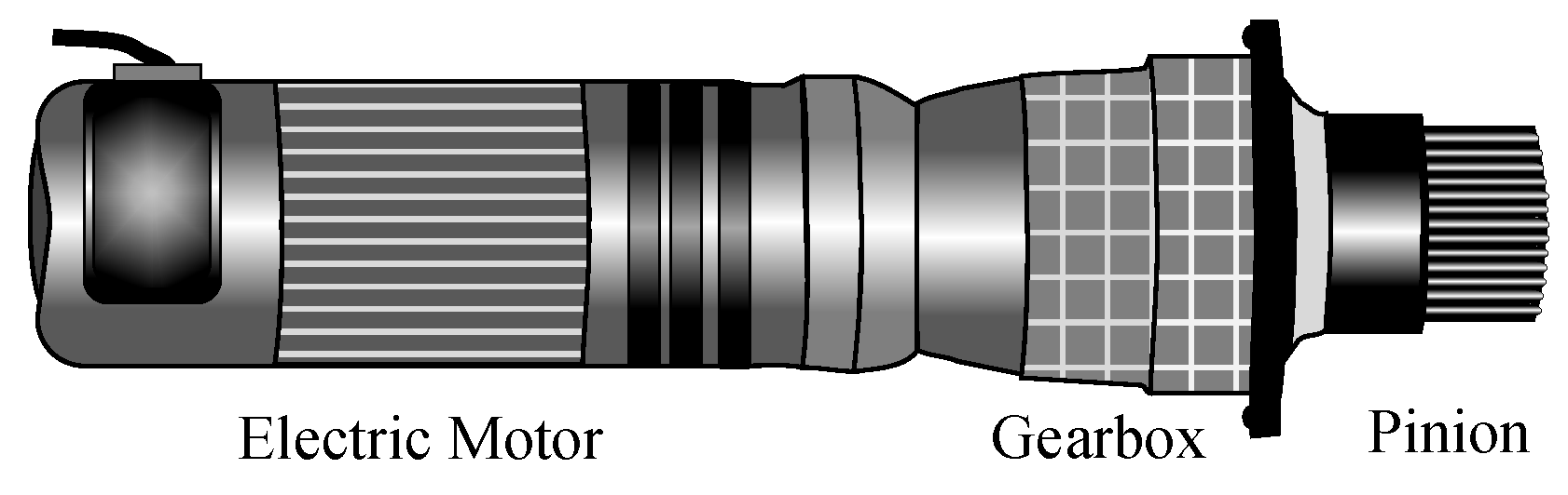
Electric actuators for pitch, as well as yaw systems, consist of an electric motor, a gearbox to reduce the speed and increase the torque, and a pinion that engages with a gear rim and the bearing attached to the rotor blade [17], as shown in Figure 1.

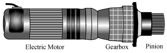
Figure 1. Schematic electrical actuator for wind turbines.

For the testing of wind turbine models, as well as control approaches, by means of simulations, it is common to use basic models for the actuators, such as, for example, first-order models (e.g., [18,19,20]) or second-order models, like [21,22,23]. For this research, the model dynamics of actuators should be more accurate.

The closed-loop dynamic model of an actuator depends on the type of the used electric motor and the internal control scheme. These aspects are analysed in the following pages.

2.2. Modelling of Permanent Magnet Synchronous Motors

In essence, any type of electric motor can be used to assemble an actuator for wind turbines. However, permanent magnet synchronous motors (PMSMs), particularly those called brushless DC motors, are preferred nowadays because they are compact, do not have rotor windings, and can provide high torque at relatively low speeds. The main drawback is the complexity and difficulty in controlling them. Hence, the work is focused on this kind of drive.

Like practically all electromechanical machines, PMSMs can be decomposed into an electrical part and a mechanical part. The dynamic model of the electrical part is created in the rotating dq-reference frame [24,25], which is obtained after the Park transformation [26], expressed by the equation

$$\begin{array}{c}\left[\begin{array}{c}{v}_d\\ v_q\end{array}\right]={\displaystyle \frac{2}{3}}\end{array}\begin{array}{c}\left[\begin{array}{ccc}\cos ({\theta }_e)& \cos ({\theta }_e-2\pi /3)& \cos ({\theta }_e-4\pi /3)\\ -\sin ({\theta }_e)& -\sin ({\theta }_e-2\pi /3)& -\sin ({\theta }_e-4\pi /3)\end{array}\right]\end{array}\left[\begin{array}{c}{v}_a\\ v_b\\ v_c\end{array}\right].$$

(1)

The vector [v_a v_b v_c]^T denotes the three-phase supply voltages, [v_d v_q]^T represents the orthogonal transformed voltages, and θ_e is the electric rotational angle. The electric dynamics can be found in practically all references on electric drives (see, e.g., [27,28,29,30]) and are given by the first-order differential equations

$${\displaystyle \frac{d{i}_d}{dt}}=(1/L_d)[-R_s\hspace{0.17em}{i}_d+L_q{\omega }_e\hspace{0.17em}{i}_q+v_d] \mathrm{and}$$

(2)

$${\displaystyle \frac{d{i}_q}{dt}}=\hspace{0.17em}(1/L_q)[-R_s\hspace{0.17em}{i}_q-(L_d\hspace{0.17em}{i}_d+{\lambda }_f)\hspace{0.17em}{\omega }_e+v_q],$$

(3)

where ω_e is the electrical speed such that for a number of pair poles p, the mechanical speed is ω_m = ω_e/p. The electrical parameters are L_q and L_d as the self-inductances of the stator windings, λ_f as the flux linkage between the stator and the rotor, and R_s as the stator resistance. The electromagnetic torque T_e is given by

$$T_e=1.5p\hspace{0.17em}[{\lambda }_f{i}_q+(L_d-L_q)\hspace{0.17em}{i}_d\hspace{0.17em}{i}_q].$$

(4)

In the case of PMSMs with nonsalient poles (surface-mounted permanent magnets), which satisfy L_d = L_q, the electromagnetic torque reduces to

$$T_e=1.5\hspace{0.17em}p\hspace{0.17em}{\lambda }_f\hspace{0.17em}{i}_q=K_T\hspace{0.17em}{i}_q.$$

(5)

In the case of a salient pole machine, the difference (L_d − L_q) can be positive, and the total torque is increased by the reluctance component. However, if the motor is well designed, L_d << L_q [31], and the torque is reduced. Thus, either for nonsalient or salient poles, it is normally desirable to regulate i_d to zero such that (5) is satisfied. This value is reached by setting i_dref = 0 in the current control system.

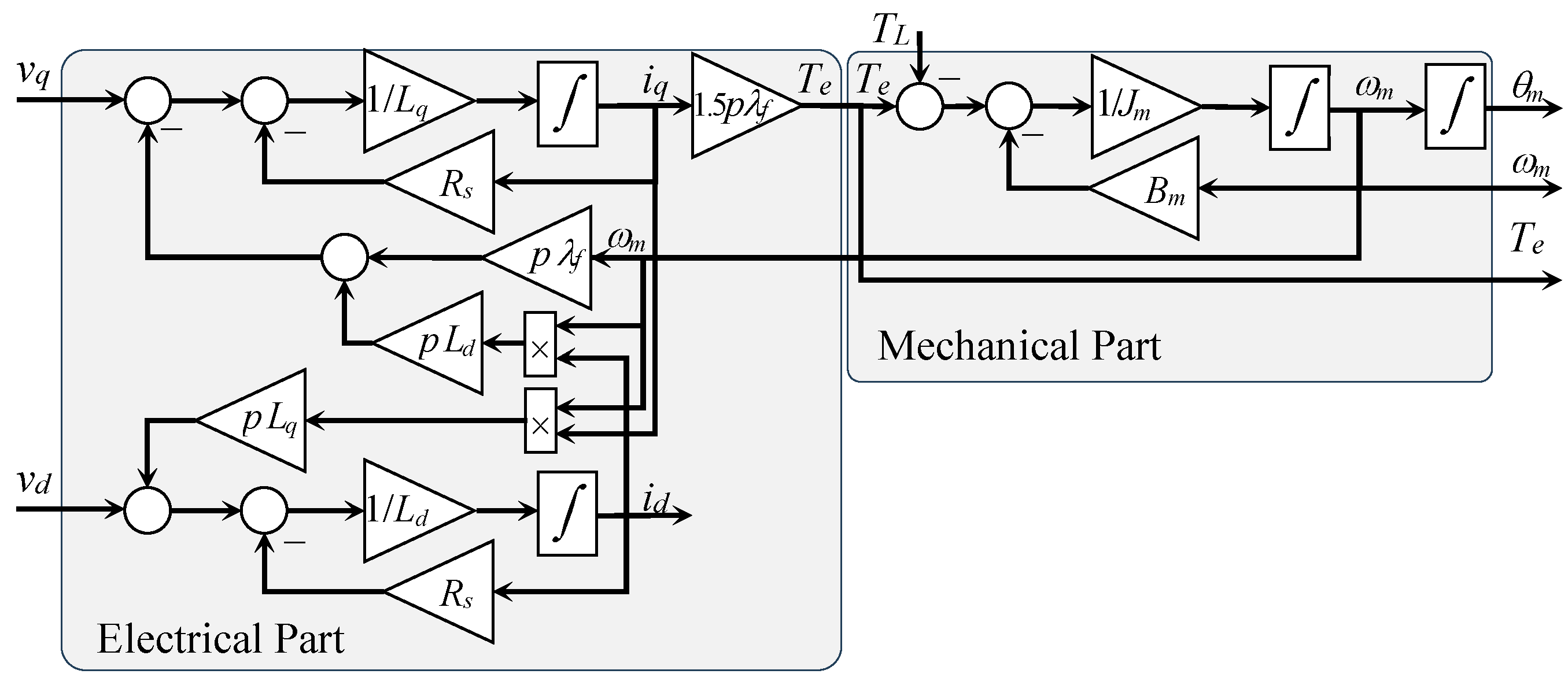
The mechanical part is described by the simple motion equation

$$J_m{\dot{\omega }}_m+B_m{\omega }_m=T_e-T_L,$$

(6)

where J_m, B_m, and T_L are the rotor mass moments of inertia, the rotor viscous friction, and the load torque, respectively. The simulation diagram is shown in Figure 2.

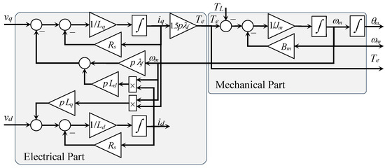
Figure 2. Schematic simulation diagram of a PMSM in the dq-reference frame.

2.3. Control of Permanent Magnet Synchronous Motors

Depending on the applications and the control objectives, there are many approaches for the control of PMSMs, such as current, torque, speed, and position control. In addition, there are several control laws and combinations of them available. There is abundant literature on the subject; for instance [27,28,32,33,34,35,36], which only mentions some of it.

The final objective of pitch actuators is to follow a position reference signal. Therefore, the presentation is limited to this aim. Moreover, the position control system of the PMSM is integrated into the actuator and, therefore, is unattainable to the user. The interest here is then to obtain the closed-loop model of the whole actuator, which is used later for the design of the synchronising control system of several actuators.

In order to obtain a position control with high performance, several nested control loops are necessary. In general, internal current control loops are implemented using PI control laws. On the other hand, there are different approaches for the position, as well as position-speed control loops. For instance, an LQR with an observer is used in [33,37]. In [38], the position control is implemented with a fuzzy logic control approach. Approaches using neural networks can be found in [39,40,41]. The current presentation uses the industrial classic control approach that combines PI controllers with feedforward terms for the current control loops, a PI controller for the speed control loop, and a nonlinear P controller with a derivative feedforward term for the position control loop.

PI and PID controllers are prone to integrator blow-up as a result of saturated actuator outputs. The problem is known as integrator windup. In the present work, all PI controllers are set with the backcalculation anti-windup mechanism [42,43,44]. This multi-controller configuration is presented in the following sections.

2.3.1. General Control Configuration

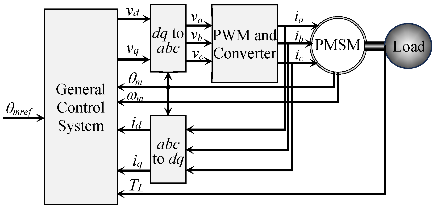
The speed (and position) control of a PMSM is difficult to implement because the only variable available is the supply voltage. Variation of the supply voltage is usually accomplished by means of a converter with a pulse-width modulation (PWM) technique, as shown in Figure 3.

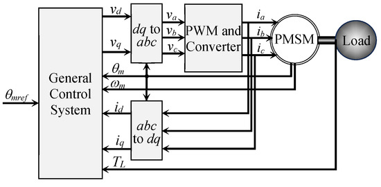
Figure 3. PMSG and the last control stage.

This work does not cover the many converter types and control strategies (see, e.g., [45,46] for a deep study of this topic). Here, a standard three-phase, two-level bidirectional MOSFET converter with a DC link and a continuous space vector modulation (SVM) generator [47] are used.

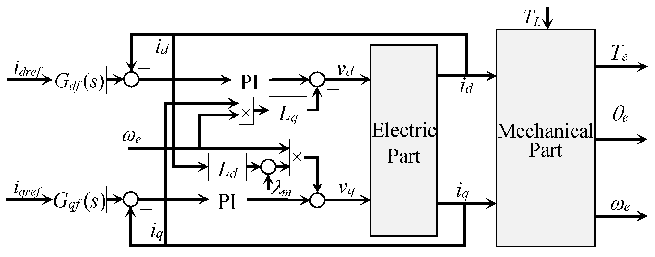
2.3.2. Current Control Loops

There is some consensus that most internal control loops include classic PI controllers for the current control, whose control signals are the voltage references for the PWM system. From Equations (2) and (3), it is clear that the model is nonlinear because of the cross-coupling terms (−L_q i_q ω_e) in (2) and (L_d i_d ω_e + λ_f ω_e) in (3). Thus, these nonlinearities can be compensated by adding these terms to the PI controllers in a feedforward form, namely

$$v_d(t)=K_{pd}(i_{dreff}-i_d)+K_{id}{\displaystyle {\int }_{t_0}^t(i_{dreff}-i_d)dt-L_q}{i}_q{\omega }_e, \mathrm{and}$$

(7)

$$v_q(t)=K_{pq}(i_{qreff}-i_q)+K_{iq}{\displaystyle {\int }_{t_0}^t(i_{qreff}-i_q)dt+(L_d}{i}_d+{\lambda }_f){\omega }_e.$$

(8)

Inserting (7) in (2) and (8) in (3), the linear expressions

$${\displaystyle \frac{d{i}_d}{dt}}=(1/L_d)[-R_s\hspace{0.17em}{i}_d+K_{pd}(i_{dreff}-i_d)+K_{id}{\displaystyle {\int }_{t_0}^t(i_{dreff}-i_d)dt}], \mathrm{and}$$

(9)

$${\displaystyle \frac{d{i}_q}{dt}}=\hspace{0.17em}(1/L_q)[-R_s\hspace{0.17em}{i}_q+K_{pq}(i_{qreff}-i_q)+K_{iq}{\displaystyle {\int }_{t_0}^t(i_{qreff}-i_q)dt}]$$

(10)

are obtained. Hence, the PI controllers with nonlinear feedforward terms also act as decouplers. By means of the Laplace transform, the transfer functions

$${\displaystyle \frac{I_d(s)}{I_{dreff}(s)}}={\displaystyle \frac{(1/L_d)(K_{pd}s+K_{id})}{s^2+[(R_s+K_{pd})/L_d]s+K_{id}/L_d}}, \mathrm{and}$$

(11)

$${\displaystyle \frac{I_q(s)}{I_{qreff}(s)}}={\displaystyle \frac{(1/L_q)(K_{pq}s+K_{iq})}{s^2+[(R_s+K_{pq})/L_q]s+K_{iq}/L_q}}$$

(12)

are attained. As can be seen, the PI controllers introduce one zero in the dynamics, which can be cancelled by first-order filtering of the reference signals using

$$G_{df}(s)={\displaystyle \frac{I_{dreff}(s)}{I_{dref}(s)}}={\displaystyle \frac{K_{id}/K_{pd}}{s+K_{id}/K_{pd}}}, \mathrm{and} G_{qf}(s)={\displaystyle \frac{I_{qreff}(s)}{I_{qref}(s)}}={\displaystyle \frac{K_{iq}/K_{pq}}{s+K_{iq}/K_{pq}}}.$$

(13)

This leads to

$${\displaystyle \frac{I_d(s)}{I_{dref}(s)}}={\displaystyle \frac{K_{id}/L_d}{s^2+[(R_s+K_{pd})/L_d]s+K_{id}/L_d}}, \mathrm{and}$$

(14)

$${\displaystyle \frac{I_q(s)}{I_{qref}(s)}}={\displaystyle \frac{K_{iq}/L_q}{s^2+[(R_s+K_{pq})/L_q]s+K_{iq}/L_q}}.$$

(15)

Consequently, by specifying natural frequencies ω_nd and ω_nq, as well as damping coefficients ζ_d and ζ_q for the inner closed loop, the controller parameters can be calculated as

$$K_{id}=L_d{\omega }_{nd}^2,K_{iq}=L_q{\omega }_{nq}^2,K_{pd}=2{\zeta }_d{\omega }_{nd}{L}_d-R_s,\mathrm{and} K_{pq}=2{\zeta }_q{\omega }_{nq}{L}_q-R_s.$$

(16)

It is very important to mention that the first-order filters have time constants defined by the controller gains, i.e., τ_d = K_pd/K_id and τ_q = K_pq/K_iq. Thus, some combinations of controller gains can make the control system too slow and therefore completely ineffective. This introduces constraints in the search for controller parameters.

The natural frequency of a second-order system fixes the settling time of the closed-loop system. A fast response is of interest for wind turbine applications. The damping coefficients are commonly chosen between 0.707 and 1 in order to obtain a practically non-oscillatory response. The natural frequency is often taken as a tenth of the natural frequency of the current control loop. The current control loops are schematised in Figure 4.

Figure 4. Block diagram of the current control system.

Finally, the transfer function (15) is now rewritten as

$${\displaystyle \frac{I_q(s)}{I_{qref}(s)}}={\displaystyle \frac{a_{i2}}{s^2+a_{i1}\hspace{0.17em}s+a_{i2}}},$$

(17)

where $a_{i1}=(R_s+K_{pq})/L_q$ and $a_{i2}=K_{iq}/L_q$.

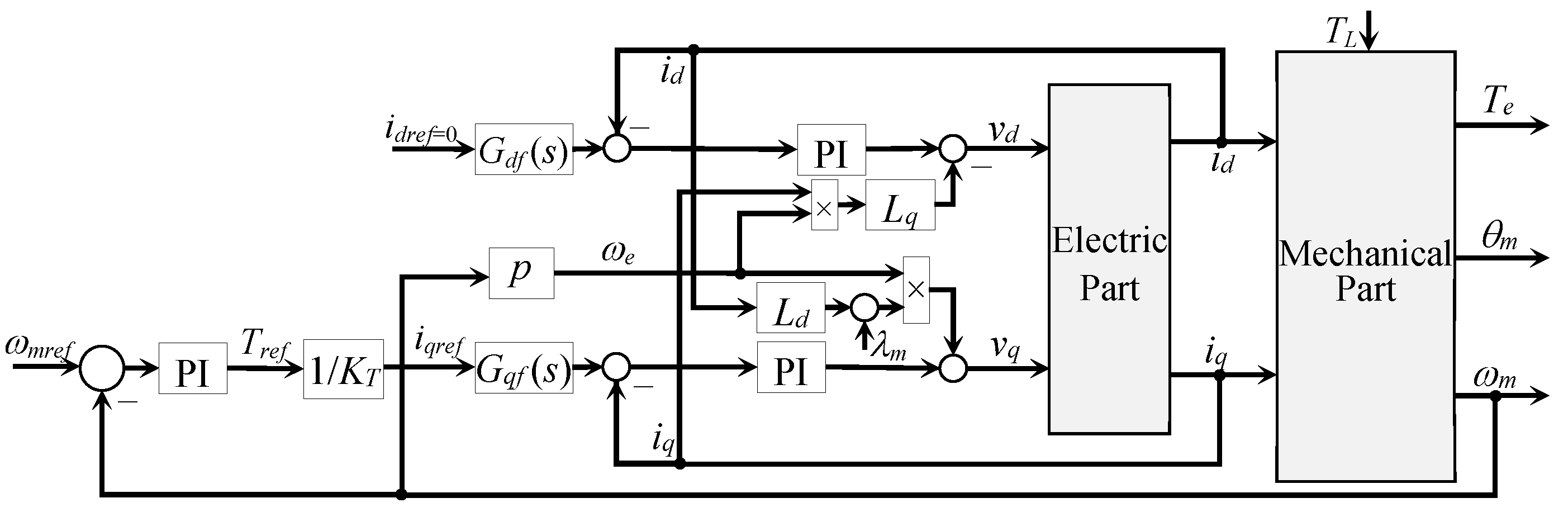
2.3.3. In-Between Speed Control Loop

Although it is possible to implement the position control loop directly in cascade configuration with the current control loops, it is common to introduce a speed controller between these control loops. The speed control loop takes place on the mechanical subsystem, and, therefore, it provides additional robustness against variations of the electrical parameters, which can change because of temperature and/or operational conditions.

As is described in Section 2.2, the d-axis current component is regulated to zero. Thus, the speed control loop provides the current reference for the q-axis current component. A PI control loop is commonly used as a speed controller, i.e.,

$$T_{eref}(t)=K_{p\omega }(b\hspace{0.17em}{\omega }_{mreff}-{\omega }_m)+K_{i\omega }{\displaystyle {\int }_{t_0}^t({\omega }_{mreff}-{\omega }_m)dt},$$

(18)

where b is the set point proportional weight. This weight is used to reduce the overshot caused by abrupt setpoint changes. The extreme choice b = 0 is chosen to avoid the proportional kick [48]. The reference i_qref for the next control loop is obtained from (5) as

$$i_{qref}={\displaystyle \frac{T_{eref}}{1.5\hspace{0.17em}p\hspace{0.17em}{\lambda }_f}}=(1/K_T)\hspace{0.17em}{T}_{eref}.$$

(19)

As T_eref, the rated torque of the motor is used, and ω_mref is provided by the position controller. The cascade control system is described in Figure 5.

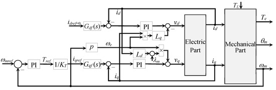
Figure 5. Block diagram of the cascade speed–current control system.

It must be remarked here that it is normal to use the electrical variables θ_e and ω_e. However, the final interest in the application is the mechanical variables of the actuators that are passed to the wind turbine. For this reason, it is preferred to use directly the mechanical variables. The relationship between both is the number of pole pairs p, namely, ω_e = p ω_m and θ_e = p θ_m.

The transfer function of the new closed-loop system is obtained from the Laplace transform of (5) and (6). Hence, one becomes

$${\Omega }_m(s)={\displaystyle \frac{(1/J_m)}{s+B_m/J_m}}{K}_T{I}_q(s)-{\displaystyle \frac{(1/J_m)}{s+B_m/J_m}}{\mathrm{T}}_L(s),$$

(20)

where Ω_m(s) and T_L(s) are the Laplace transforms of ω_m and T_L, respectively.

Introducing (17) into (20) and defining b_m1 = 1/J_m and a_m1 = B_m/J_m, the mechanical speed

$${\Omega }_m(s)={\displaystyle \frac{b_{m1}\hspace{0.17em}{K}_T}{s+a_{m1}}}{\displaystyle \frac{a_{i2}}{s^2+a_{i1}\hspace{0.17em}s+a_{i2}}}{I}_{qref}(s)-{\displaystyle \frac{b_{m1}}{s+a_{m1}}}{\mathrm{T}}_L(s),$$

(21)

is obtained. Since I_qref = T_ereff/K_T, (20) can be written as

$${\Omega }_m(s)={\displaystyle \frac{b_{m1}}{s+a_{m1}}}\hspace{0.17em}{\displaystyle \frac{a_{i2}}{s^2+a_{i1}\hspace{0.17em}s+a_{i2}}}{\mathrm{T}}_{qref}(s)-{\displaystyle \frac{b_{m1}}{s+a_{m1}}}{\mathrm{T}}_L(s),$$

(22)

and T_eref(s) is achieved by the Laplace transform of (18) and rewriting, i.e.,

$${\mathrm{T}}_{eref}(s)={\displaystyle \frac{b\hspace{0.17em}{K}_{p\omega }\hspace{0.17em}s+K_{i\omega }}{s}}{\Omega }_{mreff}(s)-{\displaystyle \frac{b\hspace{0.17em}{K}_{p\omega }\hspace{0.17em}s+K_{i\omega }}{s}}{\Omega }_m(s).$$

(23)

From (22) and (23), it follows that

$${\Omega }_m(s)={\displaystyle \frac{b_{m1}{a}_{i2}(b\hspace{0.17em}{K}_{p\omega }\hspace{0.17em}s+K_{i\omega })\hspace{0.17em}{\Omega }_{mreff}(s)-b_{m1}s(s^2+a_{i1}\hspace{0.17em}s+a_{i2}){\mathrm{T}}_L(s)}{s(s+a_{m1})(s^2+a_{i1}\hspace{0.17em}s+a_{i2})+b_{m1}{a}_{i2}(b\hspace{0.17em}{K}_{p\omega }\hspace{0.17em}s+K_{i\omega })}}.$$

(24)

Notice that the speed PI controller introduces a zero at s = −Kiω/(b K_pω). Hence, it is now cancelled, like for current controllers by the first-order filter with unity gain

$${\Omega }_{mreff}(s)={\displaystyle \frac{K_{i\omega }}{b\hspace{0.17em}{K}_{p\omega }\hspace{0.17em}s+K_{i\omega }}}{\Omega }_{mref}(s).$$

(25)

Thus, the final speed output of the closed-loop system can be described by

$${\Omega }_m(s)=G_s(s){\Omega }_{mreff}(s)-G_T(s){\mathrm{T}}_L(s),$$

(26)

where G_s(s) and G_T(s) are described by

$$G_s(s)={\displaystyle \frac{b_{m1}{a}_{i2}{K}_{i\omega }\hspace{0.17em}}{s(s+a_{m1})(s^2+a_{i1}\hspace{0.17em}s+a_{i2})+b_{m1}{a}_{i2}(b\hspace{0.17em}{K}_{p\omega }\hspace{0.17em}s+K_{i\omega })}}, \mathrm{and}$$

(27)

$$G_T(s)={\displaystyle \frac{b_{m1}\hspace{0.17em}s\hspace{0.17em}(s^2+a_{i1}\hspace{0.17em}s+a_{i2})}{s(s+a_{m1})(s^2+a_{i1}\hspace{0.17em}s+a_{i2})+b_{m1}{a}_{i2}(b\hspace{0.17em}{K}_{p\omega }\hspace{0.17em}s+K_{i\omega })}},$$

(28)

respectively.

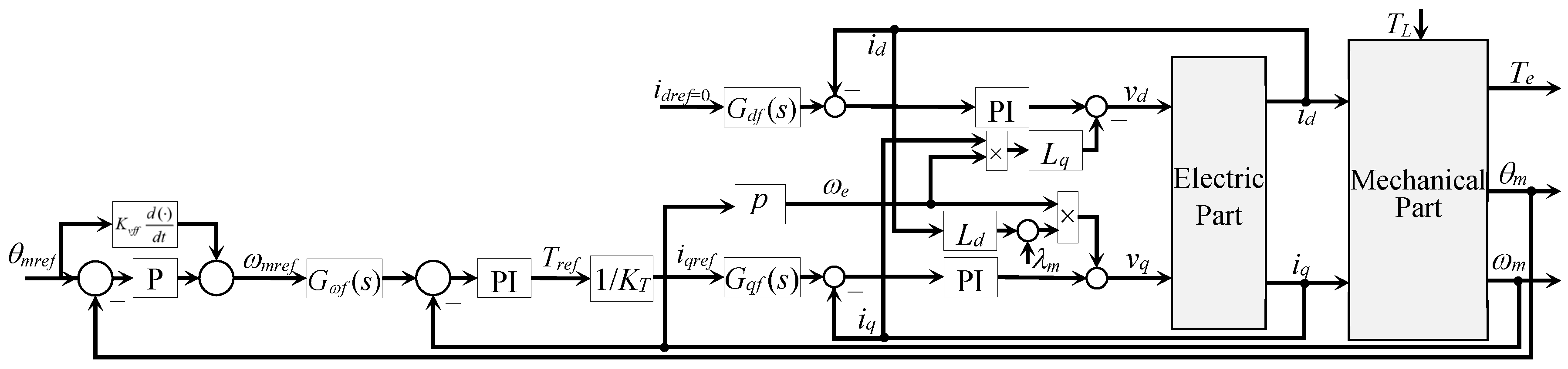
2.3.4. Position Control Loop

In the presence of a load torque T_L and without a speed controller, the position controller has to provide the integral action in order to eliminate load disturbances. It is normally arranged by a PID controller, where its derivative part also acts like a proportional term of a speed controller.

If a PI controller for speed is included, then it contributes to the integral action, and the position control can be simplified using a proportional control law. However, this configuration is slow to transmit fast position changes to the speed controller because the speed command takes place once the position error arises. Hence, the control behaviour can be improved by injecting the required speed directly into the speed control loop in a feedforward manner [49]. This feedforward–feedback configuration for the position control loop is shown in Figure 6.

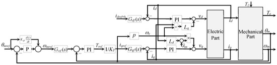
Figure 6. Block diagram of the position–speed–current control system.

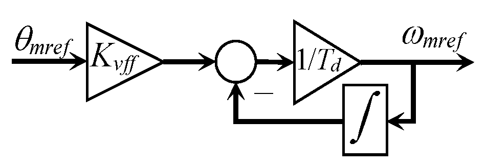
An ideal derivative operator is an acausal system and cannot be physically implemented. Hence, an estimate of the derivative term is used. The derivative feedforward controller is constructed by low-pass filtering the ideal derivative [50] according to Figure 7.

Figure 7. Estimator for the derivative term.

The transfer function of this derivative estimator is given by

$$G_{der}(s)={\displaystyle \frac{K_{vff}\hspace{0.17em}s}{1+T_d\hspace{0.17em}s}},$$

(29)

where 1/T_d is the corner frequency from which the amplitude is maintained constant.

The proportional controller can be improved using a nonlinear adaptive gain [51,52,53] given by

$$K_{p\theta }=K_{p1}+K_{p2}[1-\mathrm{sech}(K_{p3}e(t))].$$

(30)

When the control error e(t) is large, then K_pθ = K_p1 + K_p2, and in the case that e(t) is small, the gain becomes K_pθ = K_p1. The rate of change from K_p1 + K_p2, to K_p1 is fixed by K_p3.

The control law for the position controller is given by

$${\omega }_{mref}(t)=K_{p\theta }[{\theta }_{mref}(t)-{\theta }_m(t)]+K_{vff}{\displaystyle \frac{d{\theta }_{mref}(t)}{dt}},$$

(31)

whose Laplace transform leads to

$${\Omega }_{mref}(s)=(K_{p\theta }+K_{vff}s)\hspace{0.17em}{\Theta }_{mref}(s)-K_{p\theta }\hspace{0.17em}{\Theta }_m(s),$$

(32)

where Θ(s) is the Laplace transform of θ(t). Considering Ω(s) = s Θ, it follows that

$${\Omega }_{mref}(s)=(K_{p\theta }+K_{vff}s)\hspace{0.17em}{\Theta }_{mref}(s)-K_{p\theta }\hspace{0.17em}(1/s)\hspace{0.17em}{\Omega }_m(s),$$

(33)

and inserting (33) into (26) for Ω_m(s) = s Θ_m(s), it follows that

$${\Theta }_m(s)={\displaystyle \frac{\hspace{0.17em}(K_{p\theta }+K_{vff}s)G_s(s)}{s+G_s(s)K_{p\theta }}}\hspace{0.17em}\hspace{0.17em}{\Theta }_{mref}(s)-{\displaystyle \frac{G_T(s)}{s+G_s(s)K_{p\theta }}}{\mathrm{T}}_L(s).$$

(34)

For G_s(s) = B_s(s)/A_s(s) and G_T(s) = B_T(s)/A_s(s), (34) turns into

$${\Theta }_m(s)={\displaystyle \frac{\hspace{0.17em}(K_{p\theta }+K_{vff}s)B_s(s)}{s\hspace{0.17em}{A}_s(s)+B_s(s)K_{p\theta }}}\hspace{0.17em}\hspace{0.17em}{\Theta }_{mref}(s)-{\displaystyle \frac{B_T(s)}{s\hspace{0.17em}{A}_s(s)+B_s(s)K_{p\theta }}}{\mathrm{T}}_L(s).$$

(35)

The steady-state behaviour of the position closed-loop system for step reference and load, which means that Θ_mref(s) = Θ_mref0/s and T_L(s) = T_L0/s, is obtained from

$$\underset{t\to \infty }{lim}{\theta }_m(t)=\underset{s\to 0}{lim} s\hspace{0.17em}{\Theta }_m(s),$$

(36)

for (34), namely

$$\begin{array}{l}\underset{t\to \infty }{lim}{\theta }_m(t)=\underset{s\to 0}{lim} s\hspace{0.17em}\left[{\displaystyle \frac{\hspace{0.17em}(K_{p\theta }+K_{vff}s)B_s(s)}{s\hspace{0.17em}{A}_s(s)+B_s(s)K_{p\theta }}}\hspace{0.17em}\hspace{0.17em}{\displaystyle \frac{{\Theta }_{mref0}}{s}}-{\displaystyle \frac{B_T(s)}{s\hspace{0.17em}{A}_s(s)+B_s(s)K_{p\theta }}}{\displaystyle \frac{{\mathrm{T}}_{L0}}{s}}\right],\\ \underset{t\to \infty }{lim}{\theta }_m(t)=\underset{s\to 0}{lim}\hspace{0.17em}\left[{\displaystyle \frac{\hspace{0.17em}(K_{p\theta }+K_{vff}s)B_s(s)}{s\hspace{0.17em}{A}_s(s)+B_s(s)K_{p\theta }}}\hspace{0.17em}\hspace{0.17em}{\Theta }_{mref0}-{\displaystyle \frac{B_T(s)}{s\hspace{0.17em}{A}_s(s)+B_s(s)K_{p\theta }}}{\mathrm{T}}_{L0}\right],\\ \underset{t\to \infty }{lim}{\theta }_m(t)={\displaystyle \frac{\hspace{0.17em}{K}_{p\theta }{B}_s(0)}{B_s(0)K_{p\theta }}}\hspace{0.17em}\hspace{0.17em}{\Theta }_{mref0}-{\displaystyle \frac{B_T(0)}{B_s(0)K_{p\theta }}}{\mathrm{T}}_{L0}\hspace{0.17em}.\end{array}$$

(37)

From (28), the numerator is B_T(0) = 0, and then

$$\underset{t\to \infty }{lim}{\theta }_m(t)=\hspace{0.17em}{\Theta }_{mref0},$$

(38)

which means that the steady-state error is zero and the load torque disturbance is completely rejected.

Another important reflection is concluded from the denominators of (27) and (34). The order of the position closed-loop control system is five. Hence, it is not possible to assume a priori that the actuator can be approximated by a first- or second-order system. It should be checked that the other modes can be neglected.

2.3.5. Example of a PMSM Position Control

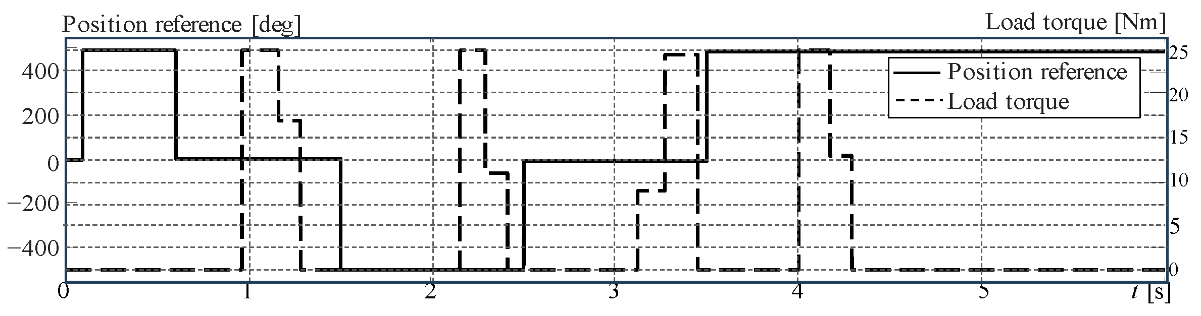
In order to illustrate the behaviour of the position control of a PMSM, the well-known example described in [33] is used. This is a 14 kW PMSM that, in its original form, implements an LQ controller with a disturbance observer for the position control (without a speed controller). The disturbance observer is required to desist from integral action, which is normally not present in the LQR approach. This example is now used as a reference. The control objective is to follow a stepwise changing position reference despite a stepwise changing load torque disturbance (see Figure 8). The rotational speed is bound to a maximum of ±500 rpm.

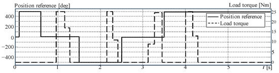
Figure 8. Reference signal and load torque used during the simulation of the position-controlled PMSM.

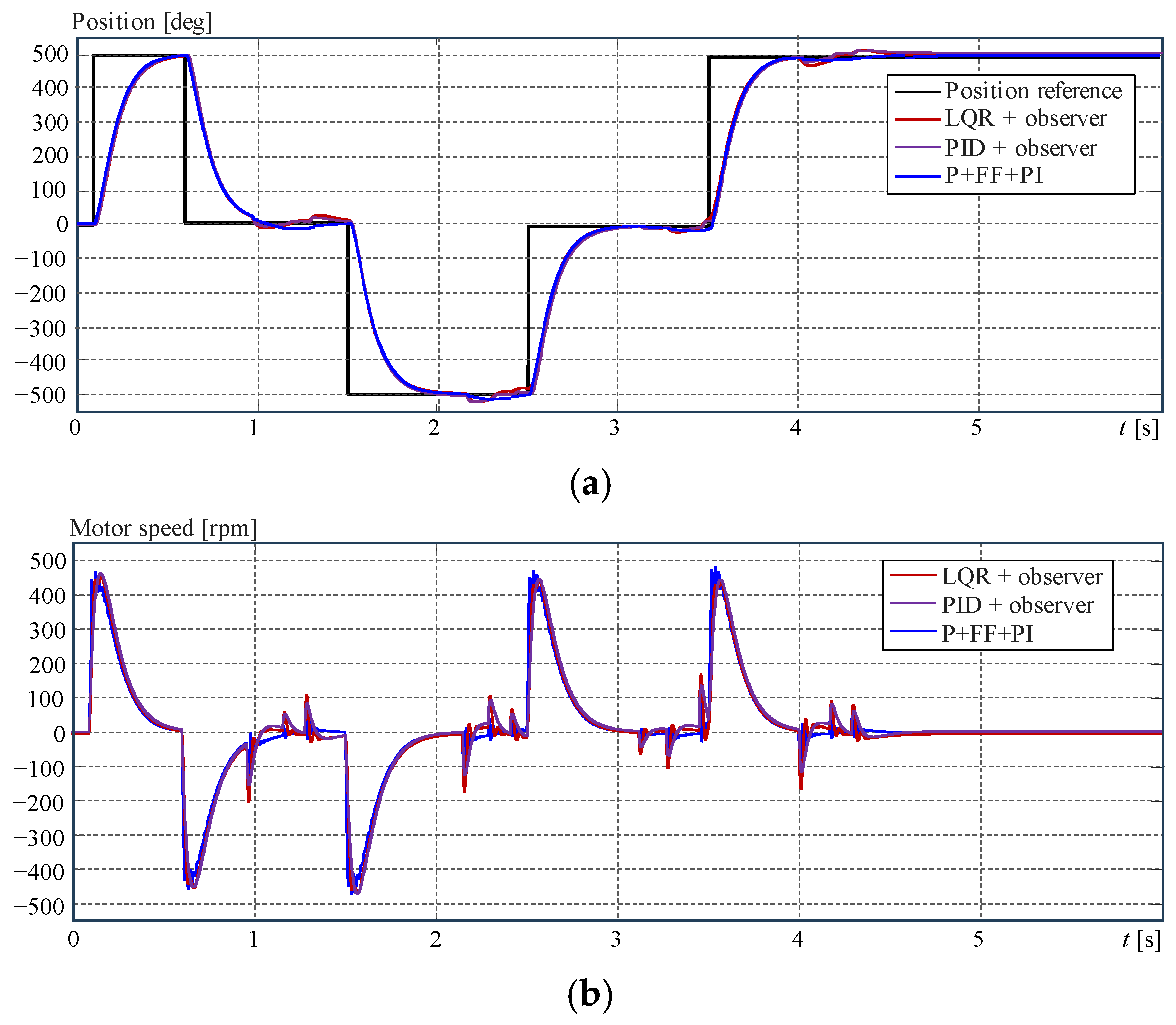
It is compared to a PI controller with a disturbance observer and with the approach described in the previous sections, which uses a P controller with a derivative feedforward term and nonlinear gain. As can be appreciated in Figure 9, the results are very similar, with a slight improvement from the last approach.

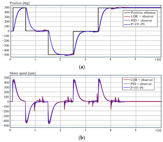
Figure 9. Simulation results for the PMSM position control systems. (a) Position output, (b) speed output.

The multi-controller approach uses standard controllers, and its advantage is that it does not depend on the accuracy of a model, in particular when the parameters change with the temperature as a PMSM does. Moreover, its distributed nature permits isolating problems and faults more easily. The drawback is given by the high number of controller parameters, which have to be jointly tuned. To this end, the methodology described in [54] has been used.

3. Synchronising Control of Several Systems

3.1. Problem Formulation

For a given number of similar transfer functions, G_i(s) = B_i(s)/[sⁿⁱ A_i(s)], with Hurwitz polynomial A_i(s) and i =1…n whose outputs y_i(t) all converge to different values, a common step input U(s), and (n − 1) identical synchronisers H(s) = Q(s)/P(s), a control system configuration should be constructed such that

$$y_1(t){|}_{t\to \infty }=y_2(t){|}_{t\to \infty }=\cdots =y_n(t){|}_{t\to \infty }=u(t){|}_{t\to \infty }.$$

(39)

The order of P(s) should be as high as necessary to satisfy (39).

This general formulation implies a very complex problem, whose analytical development can be inviable. Therefore, this study will be limited to the case that considers models with the structure given by (27) or (28).

3.2. Two-Systems Case

In the case of two systems that have to be synchronised, the proposed control system configuration is a generalisation of those presented in [10] for two simple integral systems, as shown in Figure 10.

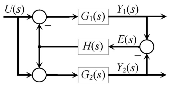
Figure 10. Control system configuration for the synchronisation of two systems.

The block diagram reduction yields

$$Y_1(s)={\displaystyle \frac{\hspace{0.17em}{G}_1(s)+2G_1(s)G_2(s)\hspace{0.17em}H(s)}{1+[G_1(s)+G_2(s)]\hspace{0.17em}H(s)}}\hspace{0.17em}\hspace{0.17em}U(s), \mathrm{and}$$

(40)

$$Y_2(s)={\displaystyle \frac{\hspace{0.17em}{G}_2(s)+2G_1(s)G_2(s)\hspace{0.17em}H(s)}{1+[G_1(s)+G_2(s)]\hspace{0.17em}H(s)}}\hspace{0.17em}\hspace{0.17em}U(s).$$

(41)

By considering G₁(s) = B₁(s)/(sⁿ₁ A₁(s), G₂(s) = B₂(s)/(sⁿ₂ A₂(s), and H(s) = Q(s)/P(s), (40) and (41) become

$$Y_1(s)={\displaystyle \frac{\hspace{0.17em}{s}^{n_2}{B}_1(s)A_2(s)P(s)+2B_1(s)B_2(s)Q(s)}{s^{n_1+n_2}{A}_1(s)A_2(s)P(s)+[s^{n_2}{B}_1(s)A_2(s)+s^{n_1}{B}_2(s)A_1(s)]Q(s)}}\hspace{0.17em}\hspace{0.17em}U(s), \mathrm{and}$$

(42)

$$Y_2(s)={\displaystyle \frac{\hspace{0.17em}{s}^{n_1}{B}_2(s)A_1(s)P(s)+2B_1(s)B_2(s)Q(s)}{s^{n_1+n_2}{A}_1(s)A_2(s)P(s)+[s^{n_2}{B}_1(s)A_2(s)+s^{n_1}{B}_2(s)A_1(s)]Q(s)}}\hspace{0.17em}\hspace{0.17em}U(s).$$

(43)

Consequently, the error between outputs is given by

$$\begin{array}{cc}\hfill E(s)& =Y_1(s)-Y_2(s)\hfill \\ & ={\displaystyle \frac{[s^{n_2}{B}_1(s)A_2(s)-s^{n_1}{B}_2(s)A_1(s)]P(s)}{s^{n_1+n_2}{A}_1(s)A_2(s)P(s)+[s^{n_2}{B}_1(s)A_2(s)+s^{n_1}{B}_2(s)A_1(s)]Q(s)}}\hspace{0.17em}\hspace{0.17em}U(s)\hfill \end{array}$$

(44)

Since (27) is of a system type equal to zero, it follows n₁ = 0 and n₂ = 0, and the error becomes

$$E(s)={\displaystyle \frac{[B_1(s)A_2(s)-B_2(s)A_1(s)]P(s)}{A_1(s)A_2(s)P(s)+[B_1(s)A_2(s)+B_2(s)A_1(s)]Q(s)}}\hspace{0.17em}\hspace{0.17em}U(s).$$

(45)

For a proportional controller, which means P(s) = 1, the error is

$$E(s)={\displaystyle \frac{[B_1(s)A_2(s)-B_2(s)A_1(s)]}{A_1(s)A_2(s)+[B_1(s)A_2(s)+B_2(s)A_1(s)]Q(s)}}\hspace{0.17em}\hspace{0.17em}U(s).$$

(46)

The steady-state error will not be zero unless both systems are identical. If the controller has an integrator, i.e., P(s) = s P₁(s), and a step input U(s) = 1/s, the error is

$$\begin{array}{cc}\hfill \underset{t\to \infty }{\lim }e(t)& =\underset{s\to 0}{\lim }sE(s)\hfill \\ & =\underset{s\to 0}{\lim }s{\displaystyle \frac{[B_1(s)A_2(s)-B_2(s)A_1(s)]\hspace{0.17em}s\hspace{0.17em}{P}_1(s)}{s\hspace{0.17em}{P}_1(s)A_1(s)A_2(s)+[B_1(s)A_2(s)+B_2(s)A_1(s)]Q(s)}}\hspace{0.17em}{\displaystyle \frac{1}{s}}\hfill \\ & =\underset{s\to 0}{\lim }{\displaystyle \frac{[B_1(s)A_2(s)-B_2(s)A_1(s)]\hspace{0.17em}s\hspace{0.17em}{P}_1(s)}{s\hspace{0.17em}{P}_1(s)A_1(s)A_2(s)+[B_1(s)A_2(s)+B_2(s)A_1(s)]Q(s)}}\hspace{0.17em}\hfill \end{array},$$

(47)

i.e.,

$$\underset{t\to \infty }{\lim }e(t)=\underset{s\to 0}{\lim }sE(s)={\displaystyle \frac{[B_1(0)A_2(0)-B_2(0)A_1(0)]·0}{[B_1(0)A_2(0)+B_2(0)A_1(0)]Q(0)}}=0.$$

(48)

Hence, both outputs are equal for two-type zero different systems if the synchroniser H(s) has integral behaviour.

The steady-state values of the outputs for n₁ = 0 and n₂ = 0 are obtained from

$$\begin{array}{cc}\hfill \underset{t\to \infty }{\lim }{y}_1(t)& =\underset{s\to 0}{\lim }s{Y}_1(s)\hfill \\ & =\underset{s\to 0}{\lim }s{\displaystyle \frac{\hspace{0.17em}{s}^{n_1}{B}_1(s)A_2(s)P(s)+2B_1(s)B_2(s)Q(s)}{s^{n_1+n_2}{A}_1(s)A_2(s)P(s)+[s^{n_2}{B}_1(s)A_2(s)+s^{n_1}{B}_2(s)A_1(s)]Q(s)}}\hspace{0.17em}{\displaystyle \frac{1\hspace{0.17em}}{s}}\hfill \\ & ={\displaystyle \frac{\hspace{0.17em}2B_1(0)B_2(0)Q(0)}{[B_1(0)A_2(0)+B_2(0)A_1(0)]Q(0)}}={\displaystyle \frac{\hspace{0.17em}2B_1(0)B_2(0)}{B_1(0)A_2(0)+B_2(0)A_1(0)}}\hfill \end{array}$$

(49)

and

$$\underset{t\to \infty }{\lim } y_2(t)={\displaystyle \frac{\hspace{0.17em}2B_1(0)B_2(0)}{B_1(0)A_2(0)+B_2(0)A_1(0)}},$$

(50)

which, in general, are different from 1. Moreover, the steady-state values of the outputs are independent of the synchronisers. Thus, the configuration in Figure 10 is unable to satisfy the last condition in (39). A solution is to scale the outputs according to the closed-loop steady-state gains, as shown in Figure 11.

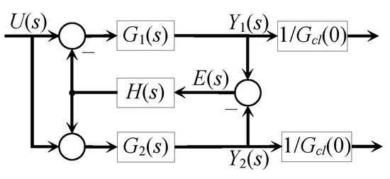
Figure 11. Modified control system configuration for the synchronisation of two systems.

3.3. Three-Systems Case

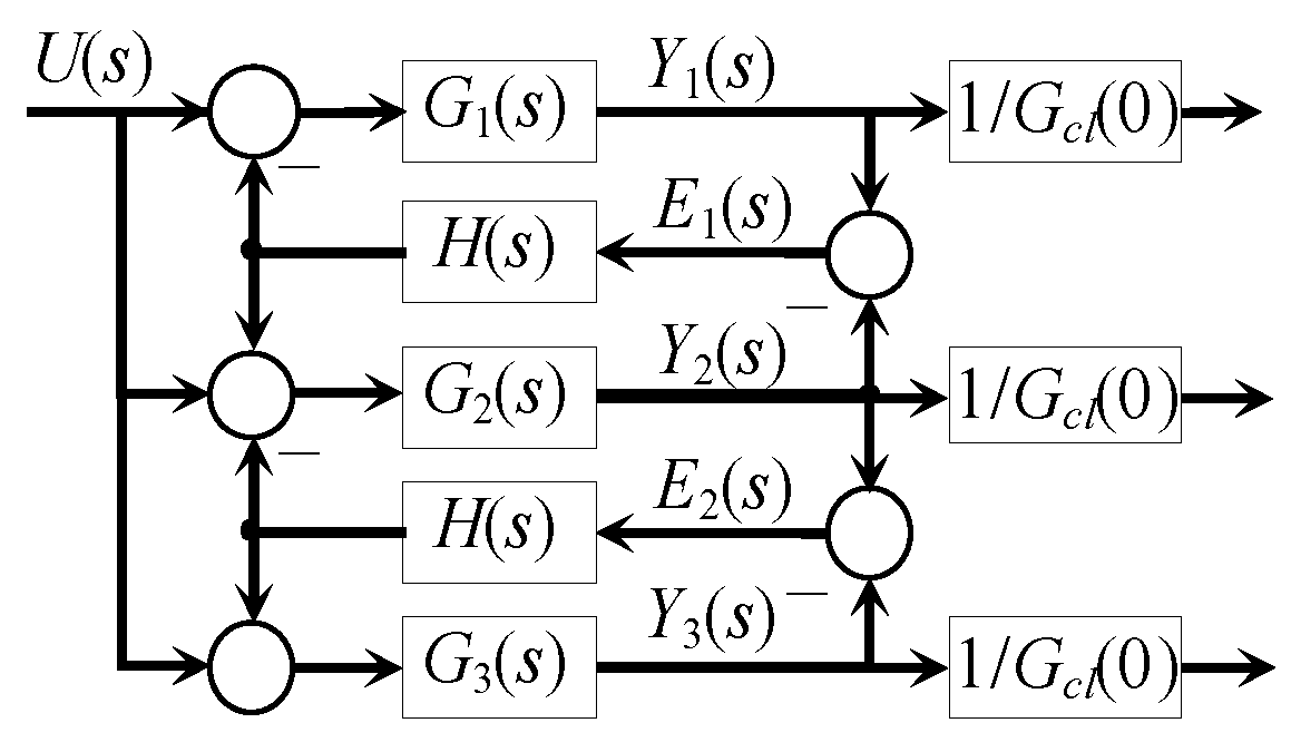
The control configuration described above for two systems is now extended to three systems. However, this configuration is a simplified version of those proposed in [10]. The extended multi-system configuration is presented in Figure 12.

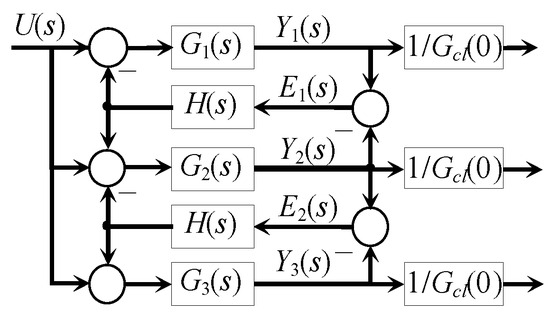
Figure 12. Control system configuration for the synchronisation of three systems.

The closed-loop outputs are obtained using block diagram reduction similar to the two-systems case. The corresponding equations are described by

$$Y_1(s)={\displaystyle \frac{G_1(s)+2G_1(s)G_2(s)\hspace{0.17em}H(s)+G_1(s)G_3(s)\hspace{0.17em}H(s)+2G_1(s)G_2(s)G_3(s)H{(s)}^2}{1+[G_1(s)+G_2(s)+G_3(s)]\hspace{0.17em}H(s)+[G_1(s)+G_2(s)]\hspace{0.17em}{G}_3(s)\hspace{0.17em}H{(s)}^2}}\hspace{0.17em}U(s),$$

(51)

$$Y_2(s)={\displaystyle \frac{G_2(s)+2G_1(s)G_2(s)\hspace{0.17em}H(s)+G_2(s)G_3(s)\hspace{0.17em}H(s)+2G_1(s)G_2(s)G_3(s)H{(s)}^2}{1+[G_1(s)+G_2(s)+G_3(s)]\hspace{0.17em}H(s)+[G_1(s)+G_2(s)]\hspace{0.17em}{G}_3(s)\hspace{0.17em}H{(s)}^2}}\hspace{0.17em}U(s), \mathrm{and}$$

(52)

$$Y_3(s)={\displaystyle \frac{G_3(s)+2G_2(s)G_3(s)\hspace{0.17em}H(s)+G_1(s)G_3(s)\hspace{0.17em}H(s)+2G_1(s)G_2(s)G_3(s)H{(s)}^2}{1+[G_1(s)+G_2(s)+G_3(s)]\hspace{0.17em}H(s)+[G_1(s)+G_2(s)]\hspace{0.17em}{G}_3(s)\hspace{0.17em}H{(s)}^2}}U(s).$$

(53)

The errors between outputs are calculated by a subtraction of (51)–(53), namely

$$E_1(s)=Y_1(s)-Y_2(s)={\displaystyle \frac{[G_1(s)-G_2(s)][1+G_3(s)\hspace{0.17em}H(s)]}{1+[G_1(s)+G_2(s)+G_3(s)]\hspace{0.17em}H(s)+[G_1(s)+G_2(s)]\hspace{0.17em}{G}_3(s)\hspace{0.17em}H{(s)}^2}}\hspace{0.17em}U(s) \mathrm{and}$$

(54)

$$E_2(s)=Y_2(s)-Y_3(s)={\displaystyle \frac{G_2(s)-G_3(s)+[2G_1(s)G_2(s)-G_1(s)G_3(s)-G_2(s)G_3(s)\hspace{0.17em}]H(s)}{1+[G_1(s)+G_2(s)+G_3(s)]\hspace{0.17em}H(s)+[G_1(s)+G_2(s)]\hspace{0.17em}{G}_3(s)\hspace{0.17em}H{(s)}^2}}\hspace{0.17em}U(s).$$

(55)

In order to analyse the steady-state errors, the definitions G₁(s) = B₁(s)/(sⁿ₁ A₁(s), G₂(s) = B₂(s)/(sⁿ₂ A₂(s), and H(s) = Q(s)/P(s) are considered. In order to simplify the notation, the argument(s) are eliminated from the equations. Hence, it follows that

$$E_1(s)={\displaystyle \frac{P\hspace{0.17em}(s^{n_2}{B}_1{A}_2-s^{n_1}{A}_1{B}_2)(s^{n_3}{A}_3+3B_{3}Q)}{s^{n_1+n_2+n_3}{A}_1{A}_2{A}_3{P}^2+Q[s^{n_2+n_3}{B}_1{A}_2{A}_3+s^{n_1+n_3}{A}_1{B}_2{A}_3]P+[s^{n_2}{B}_1{A}_2{B}_3+s^{n_1}{A}_1{B}_2{B}_3]Q^2}}\hspace{0.17em}U(s) \mathrm{and}$$

(56)

$$E_2(s)={\displaystyle \frac{P\hspace{0.17em}(s^{n_2+n_3}{B}_1{A}_2{A}_{3}P-s^{n_1+n_2}{A}_1{A}_2{B}_{3}P+s^{n_3}2B_1{B}_2{A}_{3}Q-s^{n_1+n_2}2A_1{B}_2{B}_{3}Q)}{s^{n_1+n_2+n_3}{A}_1{A}_2{A}_3{P}^2+Q(s^{n_2+n_3}{B}_1{A}_2{A}_3+s^{n_1+n_3}{A}_1{B}_2{A}_3)P+(s^{n_2}{B}_1{A}_2{B}_3+s^{n_1}{A}_1{B}_2{B}_3)Q^2}}\hspace{0.17em}U(s).$$

(57)

For n₁ = 0, n₂ = 0, n₃ = 0, and P(s) = s, (56) and (57) become

$$E_1(s)={\displaystyle \frac{s(B_1{A}_2-A_1{B}_2)(A_3+3B_{3}Q)}{s^2{A}_1{A}_2{A}_3+s\hspace{0.17em}Q\hspace{0.17em}(B_1{A}_2{A}_3+A_1{B}_2{A}_3)+(B_1{A}_2{B}_3+A_1{B}_2{B}_3)\hspace{0.17em}{Q}^2}}\hspace{0.17em}U(s), \mathrm{and}$$

(58)

$$E_2(s)={\displaystyle \frac{s\hspace{0.17em}(s\hspace{0.17em}{B}_1{A}_2{A}_3-s\hspace{0.17em}{A}_1{A}_2{B}_3+2B_1{B}_2{A}_{3}Q-2A_1{B}_2{B}_{3}Q)}{s^2{A}_1{A}_2{A}_3+s\hspace{0.17em}(B_1{A}_2{A}_3+A_1{B}_2{A}_3)Q+(B_1{A}_2{B}_3+A_1{B}_2{B}_3)Q^2}}\hspace{0.17em}U(s),$$

(59)

and then for U(s) = 1/s, the steady-state error is obtained from

$$\underset{t\to \infty }{\lim } e_1(t)=\underset{s\to 0}{\lim }s{E}_1(s)={\displaystyle \frac{(B_1{A}_2-A_1{B}_2)(A_3+3B_{3}Q)·0}{(B_1{A}_2{B}_3+A_1{B}_2{B}_3)\hspace{0.17em}{Q}^2}}=0, \mathrm{and}$$

(60)

$$\underset{t\to \infty }{\lim } e_2(t)=\underset{s\to 0}{\lim }s{E}_2(s)={\displaystyle \frac{2\hspace{0.17em}(2B_1{B}_2{A}_3-2A_1{B}_2{B}_3)·0}{(B_1{A}_2{B}_3+A_1{B}_2{B}_3)Q}}=0,$$

(61)

which means $\underset{t\to \infty }{\lim } y_1(t)=\underset{t\to \infty }{\lim } y_2(t)$, and $\underset{t\to \infty }{\lim } y_2(t)=\underset{t\to \infty }{\lim } y_3(t)$, and so $\underset{t\to \infty }{\lim } y_1(t)=\underset{t\to \infty }{\lim } y_3(t)$.

3.4. Example for the Synchronisation of Four Different Systems

For more than three systems, the analytical derivation of the output equations is very extensive and cumbersome. However, it is not difficult to verify the validity of the concept using simulations, as shown in the following example. The transfer functions are

$$G_1(s)={\displaystyle \frac{\hspace{0.17em}1.2}{s^2+2\hspace{0.17em}s+1}}, G_2(s)={\displaystyle \frac{\hspace{0.17em}1.4}{s^2+2\hspace{0.17em}s+3}}, G_3(s)={\displaystyle \frac{\hspace{0.17em}4}{s+2}}\mathrm{and} G_4(s)={\displaystyle \frac{\hspace{0.17em}0.5\hspace{0.17em}s+1}{s^3+2\hspace{0.17em}{s}^2+3\hspace{0.17em}s+1}}.$$

(62)

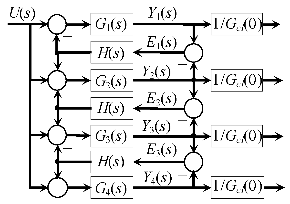
The synchronisers are defined as H(s) = 2 + 1/s. The closed-loop steady-state gain is G_cl(0) = 0.9394, and it is used to scale the outputs to the unity. The control system configuration for four plants is schematised in Figure 13.

Figure 13. Control system configuration for the synchronisation of four systems.

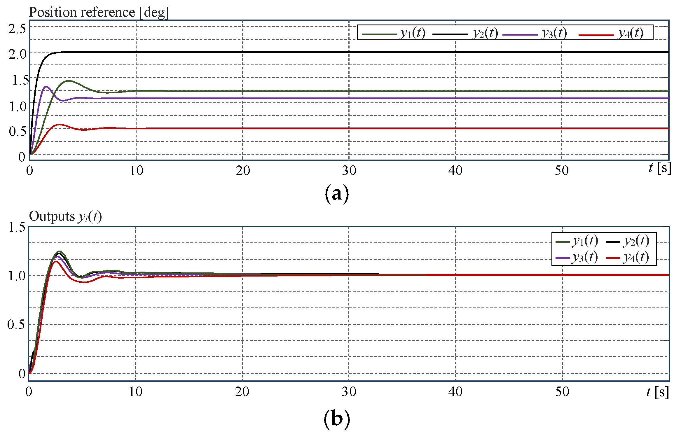
The common input is a unity step signal. The simulation results presenting the synchronised outputs are portrayed in Figure 14.

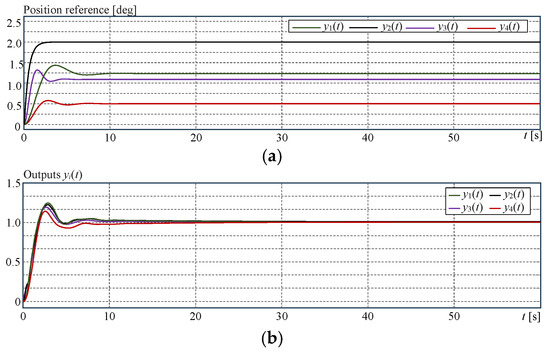
Figure 14. Simulation results of the multi-systems example. (a) Open-loop step responses. (b) Synchronised outputs.

4. Numerical Studies for Pitch Actuators in Wind Turbines

As mentioned in the Introduction, the actuator synchronisation problem can be found for wind turbines in the pitch actuator control as well as in the yaw actuator control. The present study is limited to the pitch actuator control, including the pitch actuator synchronisation in the same blade and the pitch actuator synchronisation in different blades.

4.1. Pitch Actuator Design and Model Building

The target wind turbine is a three-bladed 20-MW machine [17,55], whose maximum load moment is T_Lmax = 3762 kNm. In order to manage this large moment, three pitch actuators are necessary. The specifications for the actuator design are a pitching speed at the blade root of ω_b = 1.6667 rpm (10 deg/s) and the blade root radius r_b = 3.2 m, which is also taken as the radius of the gear rim. The radius of the pinion is chosen to be r_p = 0.2 m.

The maximum load moment is too high compared with commercial pitch actuators. Consequently, multiple pitch actuators are required to handle the load torque. The relationship between the load torque and the motor torque is given by

$$T_{Lmax}=n_a{n}_m{n}_x{T}_m,$$

(63)

where n_a is the number of actuators put into play, n_m is the gear rim ratio, and n_x is the gearbox ratio. The gear rim ratio is n_m = r_b/r_p = 3.2/0.2 = 16. On the other hand, n_x = ω_m/(n_mω_b) with ω_m as motor speed, and this leads to

$$T_{Lmax}={\displaystyle \frac{n_a{n}_m{\omega }_m{T}_m}{n_m{\omega }_b}}={\displaystyle \frac{n_a{\omega }_m{T}_m}{{\omega }_b}}.$$

(64)

Since n_a/ω_b = 3/1.6667 = 1.8 [1/rpm], (64) becomes

$$T_{Lmax}=1.8\hspace{0.17em}{\omega }_m\hspace{0.17em}{T}_m.$$

(65)

A motor of 218.9 kW is chosen with a torque of T_m = 650 Nm and a speed of ω_m = 3216.5 rpm. Hence, the maximum torque that can be applied to the blade considering three actuators is 3762018 Nm, which satisfies the maximum load torque. The rated values are also defined as steady-state values. The stationary torque difference is set to ΔT = T_e − T_L = 0.0008815. The rated line-to-line voltage is V_s = 481 V (rms) and the current is I_s = 329.51 A, with v_d = 49.6 V, v_q = 678.2 V, i_d = 233 A, and i_q = 233 A. The gearbox ratio is n_x = 120.6.

Rewriting the steady-state equations in matrix form and considering the rated values as data, the physical parameter of the motor can be calculated from

$$\left[\begin{array}{c}{L}_d\\ R_s\\ {\lambda }_f\\ B_m\end{array}\right]={\left[\begin{array}{cccc}-p{\omega }_m& i_d& 0& 0\\ p{\omega }_m{i}_d& i_q& p\omega & 0\\ 0& 0& 1.5p{i}_q& 0\\ 0& 0& 0& {\omega }_m\end{array}\right]}^{-1}\left[\begin{array}{c}{v}_d\\ v_q\\ T_m\\ \Delta T\end{array}\right].$$

(66)

By solving (66), the physical parameters are L_d = L_q = 3.474 × 10⁻⁶ H, R_s = 0.2176 Ω, λ_f = 0.4649 Wb, and B_m = 0.2969 Nm s/rad. The mass moment of inertia is calculated as J_m = 1.6134 kg m². The parameters of the other two actuators are selected within a variation range of ±10% regarding the parameters of the first actuator. All parameters are summarised in Table 1.

Table 1. Physical parameters of all three actuators and controller parameters.

Parameters	Actuator 1	Actuator 2	Actuator 3
Ld, Lq	3.4740 × 10−6 H	3.3003 × 10−6 H	5.2110 × 10−6 H
Rs	0.2176 Ω	0.2067 Ω	0.3263 Ω
λf	0.4459 Wb	0.4301 Wb	0.4816 Wb
Bm	0.2969 Nm s/rad	0.3821 Nm s/rad	0.1528 Nm s/rad
Jm	1.6134 kg m2	1.5327 kg m2	1.6457 kg m2
Steady-state speed	3216.48 rpm	3486.5 rpm	3286.98 rpm

4.2. Pitch Actuator Control System Design

As has been described in the previous section, the actuator control configuration consists of two PI current controllers with nonlinear feedforwards, one PI speed controller, and a nonlinear P position controller with derivative feedforward, i.e., there are eight parameters to be calculated and tuned. The method used for this purpose is the simulation-based multi-objective parametric optimisation (see [56] and its references for details). The optimisation objective is to minimise the square position control error without exceeding the maximum blade speed of 1.6667 rpm, which corresponds to a motor speed of 3216.48 rpm. The parameters for each individual actuator are summarised in Table 2.

Table 2. Controller parameters.

Parameters	Actuator 1	Actuator 2	Actuator 3
Current controllers	Kpd = 4.4173	Kpd = 3.9551	Kpd = 4.3940
	Kid = 8.6107	Kid = 9.1312	Kid = 7.9113
	Kpq = 0.0143	Kpq = 0.0099	Kpq = 0.0211
	Kiq = 0.7001	Kiq = 0.6906	Kiq = 0.6798
Speed controllers	Kpt = 0.9383	Kpt = 0.9364	Kpt = 0.8508
	Kit = 0.1245	Kit = 0.1241	Kit = 0.1214
Position controllers	Kp1 = 0.0604	Kp1 = 0.0043	Kp1 = 0.0421
	Kp2 = 4.5104	Kp2 = 5.0911	Kp2 = 3.9110
	Kp3 = 2.0000	Kp3 = 2.0000	Kp3 = 2.0000

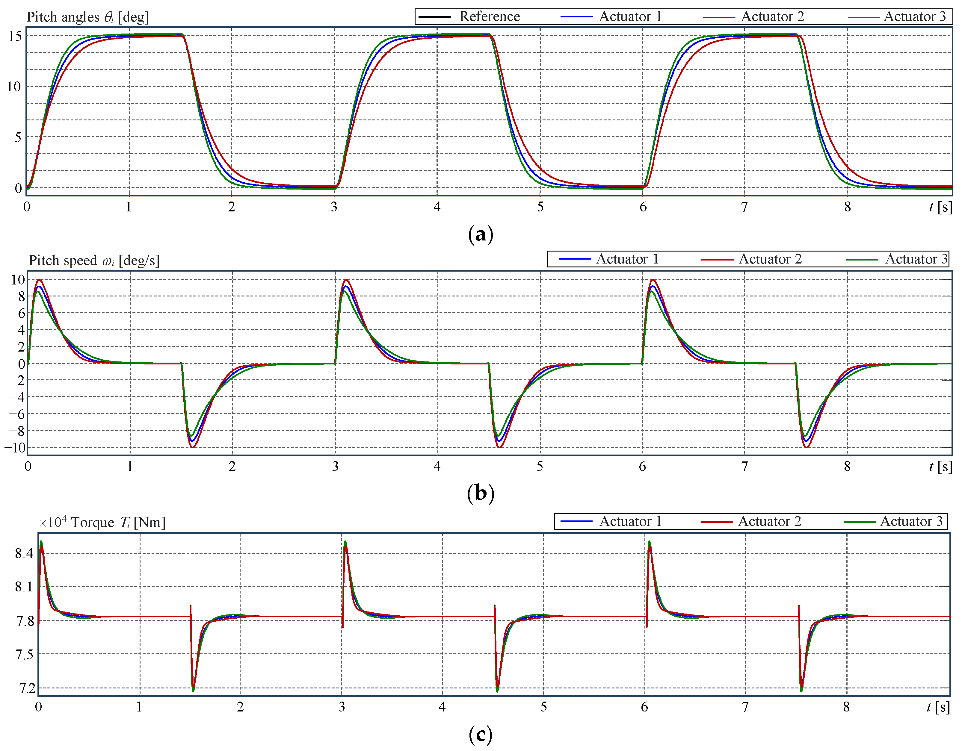
All three actuators are simulated individually following a periodic square reference signal between 0 and 15 degrees and a period of three seconds. The results are shown in Figure 15. Angles and speeds are scaled according to the gear rim ratio, and the torques correspond to the values delivered by the gearboxes.

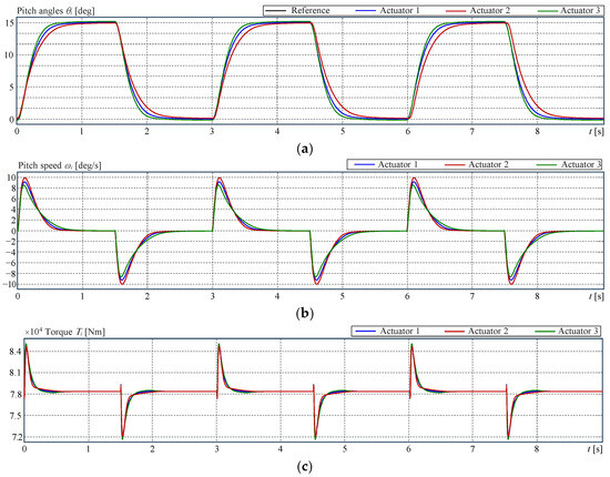
Figure 15. Simulation results for each individual pitch actuator. (a) Position (angle). (b) Speed. (c) Torque.

4.3. Example 1: Synchronised Pitch Actuator Control on the Same Blade

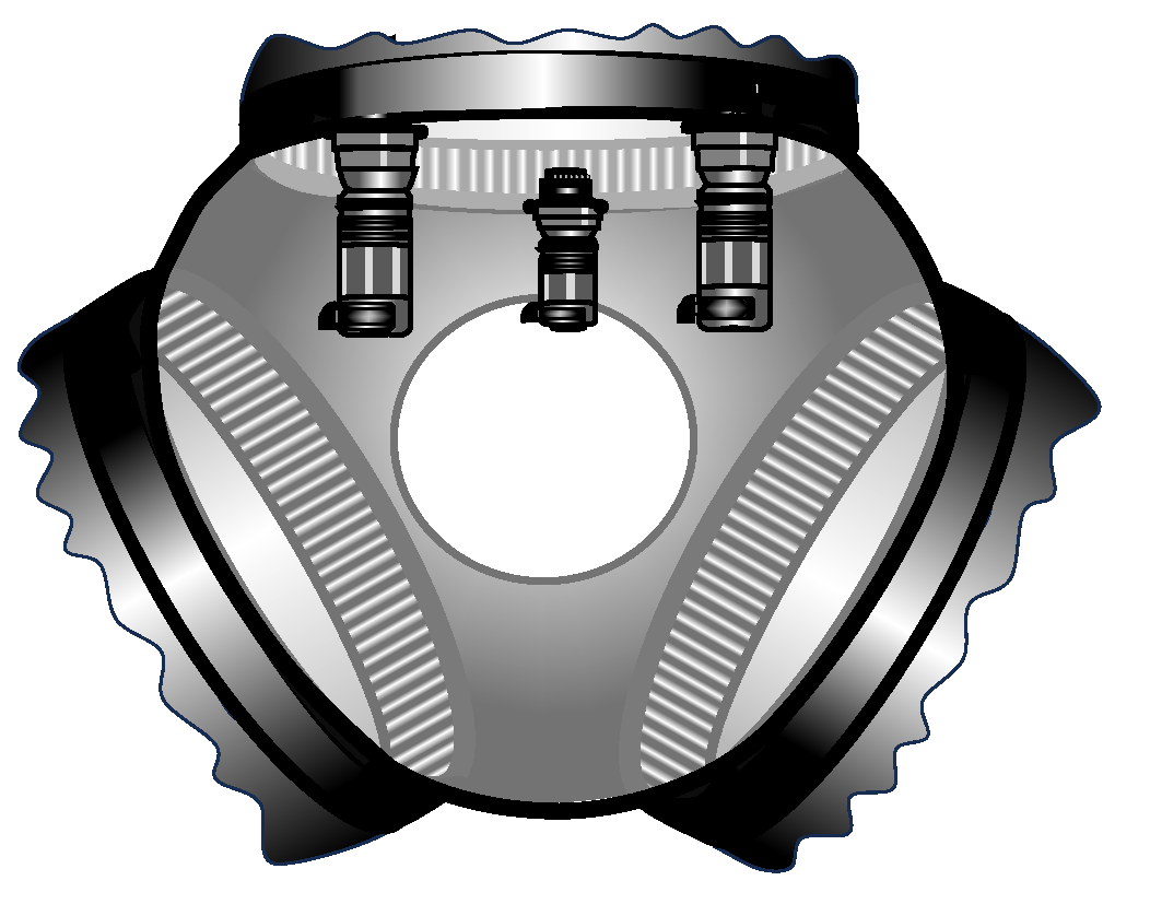
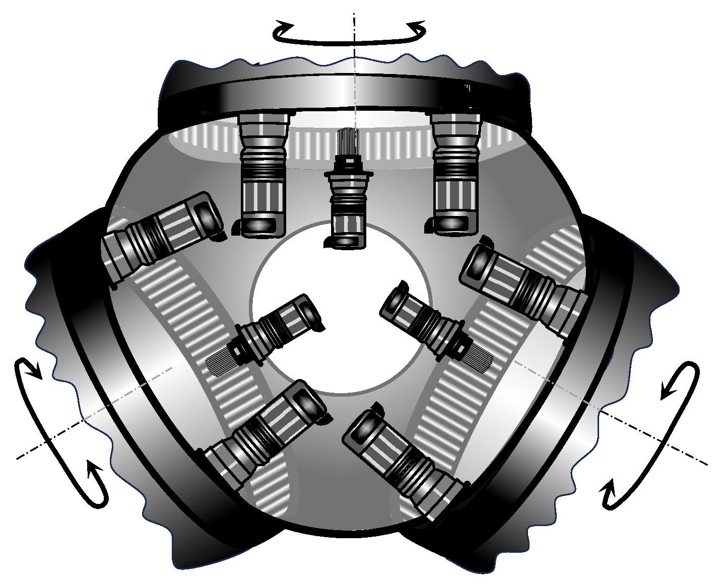
This example considers three pitch actuators attached to the same gear rim of one blade, as illustrated in Figure 16. Because the pinions are rigidly coupled to the gear rim, angles and speeds are not in the foreground. On the other hand, different torques entering the gear rim must be synchronised in order to avoid unbalanced forces acting around the bearing.

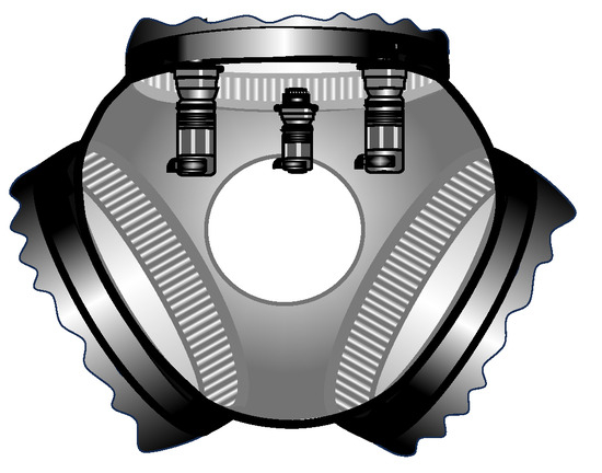
Figure 16. Three pitch actuators attached to the same gear rim.

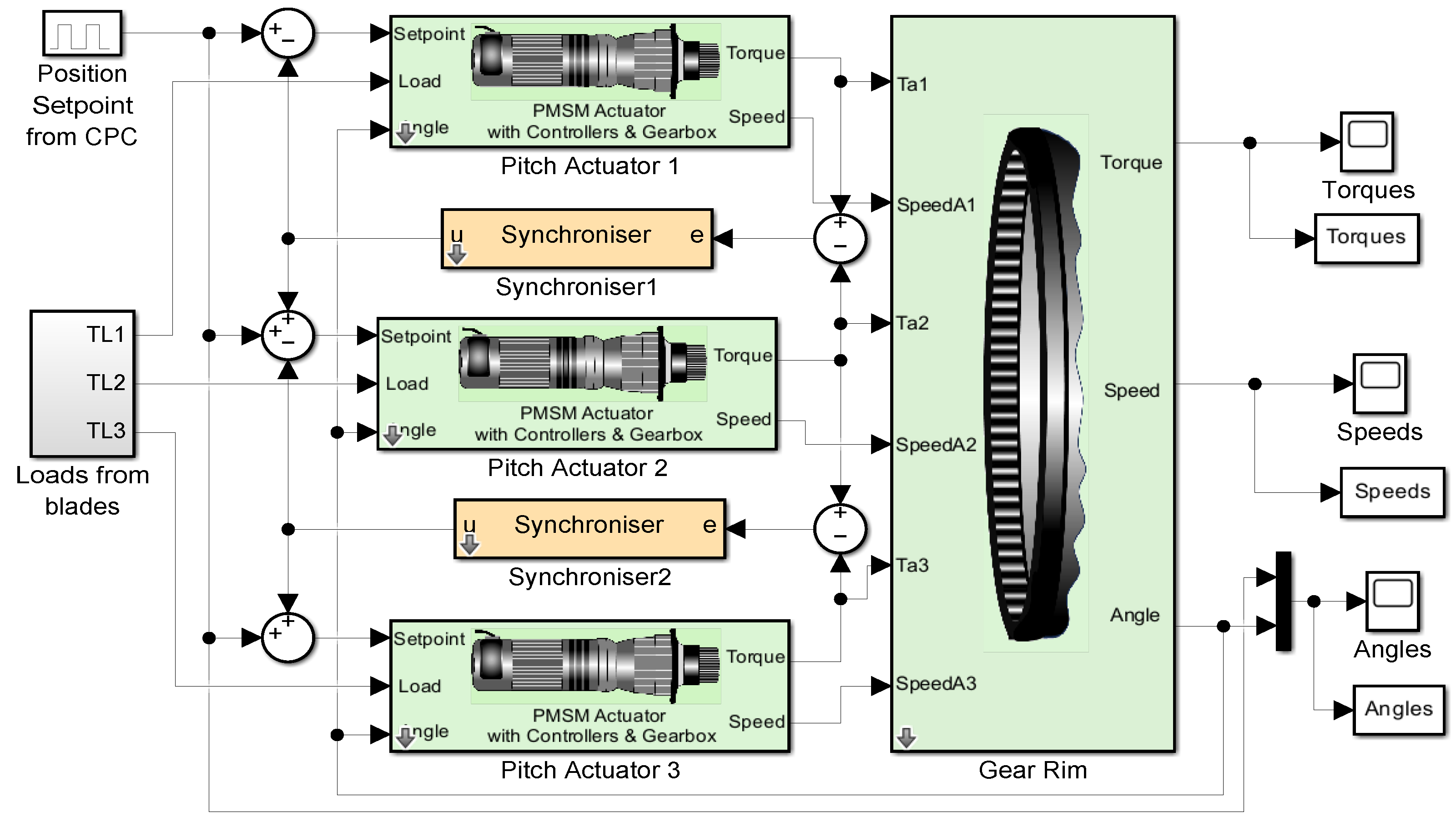
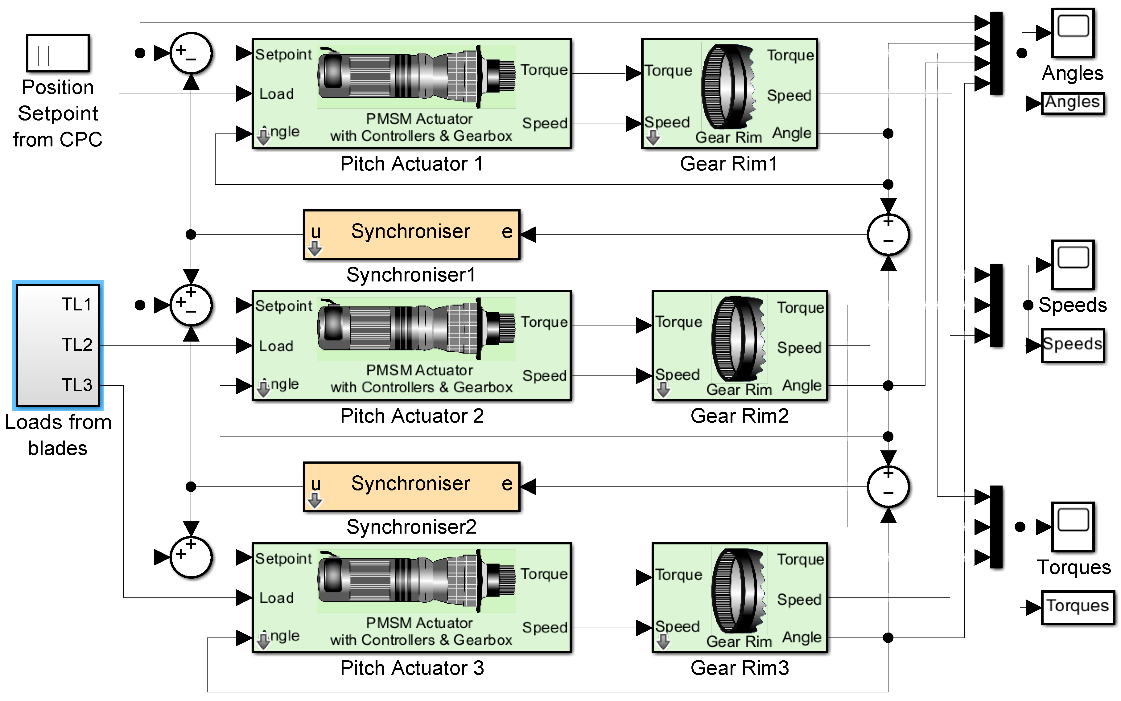
The simulation block diagram is presented in Figure 17.

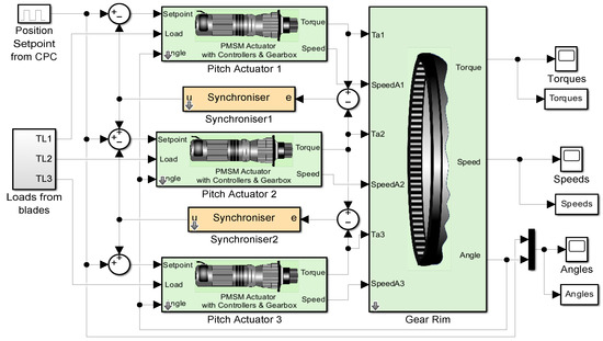
Figure 17. Simulation block diagram for the first example.

Since the pitch actuators have transfer functions of type zero (see (27)), the integral action has to be contributed by the synchronisers. Therefore, they are implemented as PI controllers according to the control law

$$H(s)=K_{ps}+{\displaystyle \frac{K_{is}}{s}}$$

(67)

with parameters K_ps = 0.5601 and K_is = 0.2206. The simulation results are shown in Figure 18.

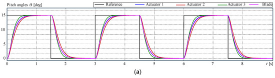
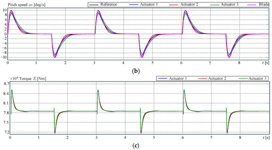
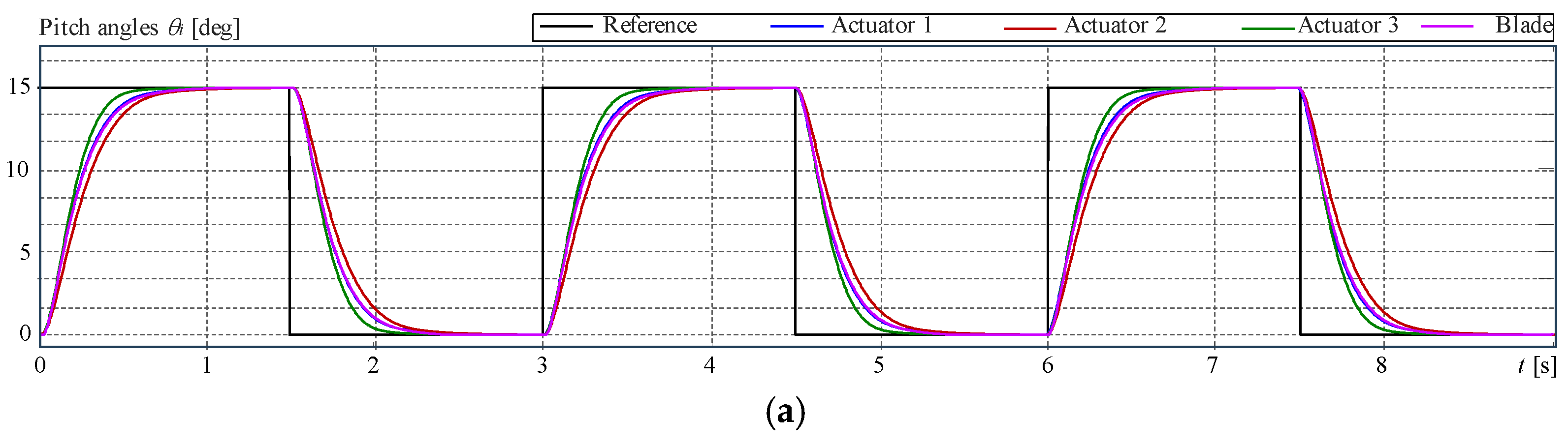
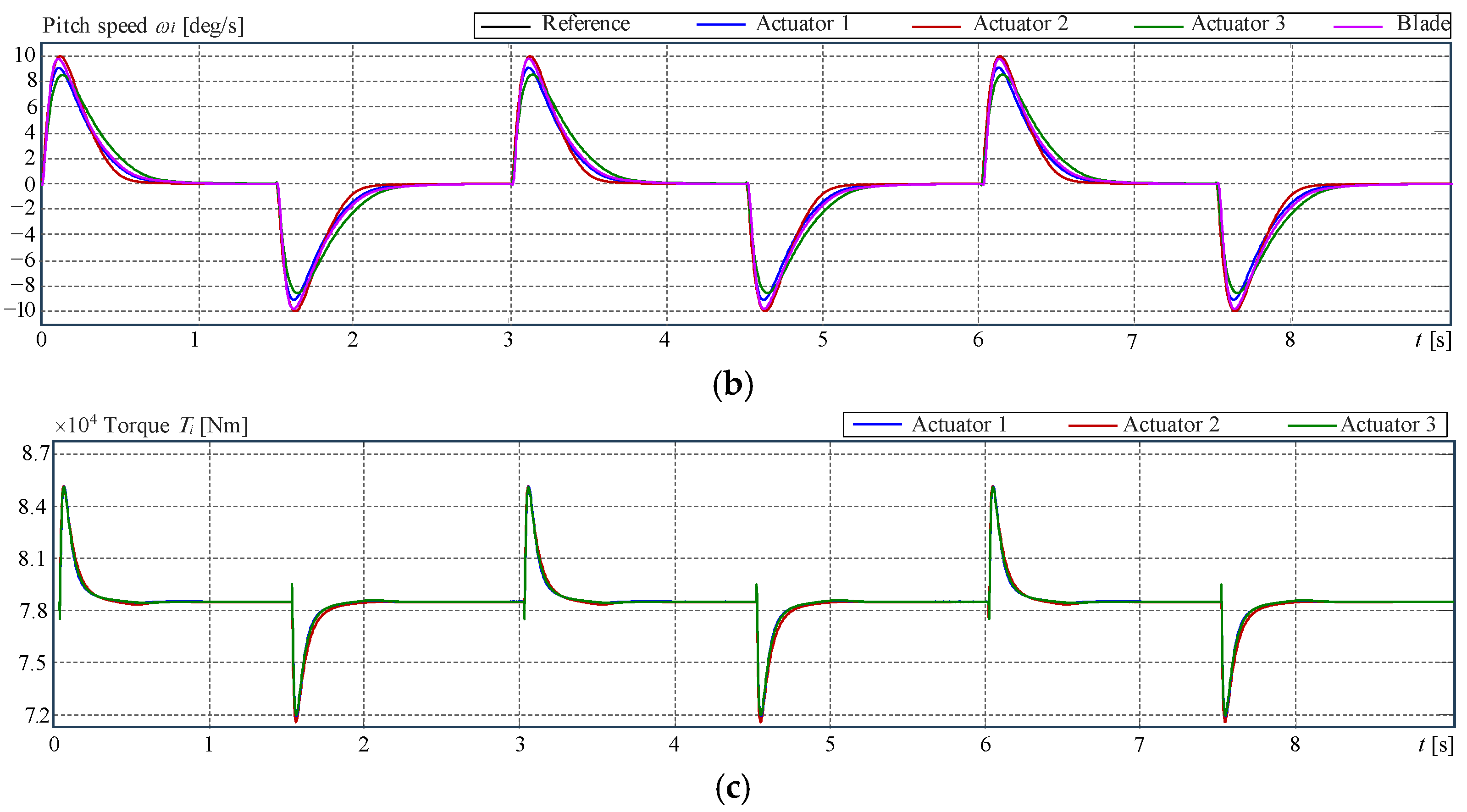
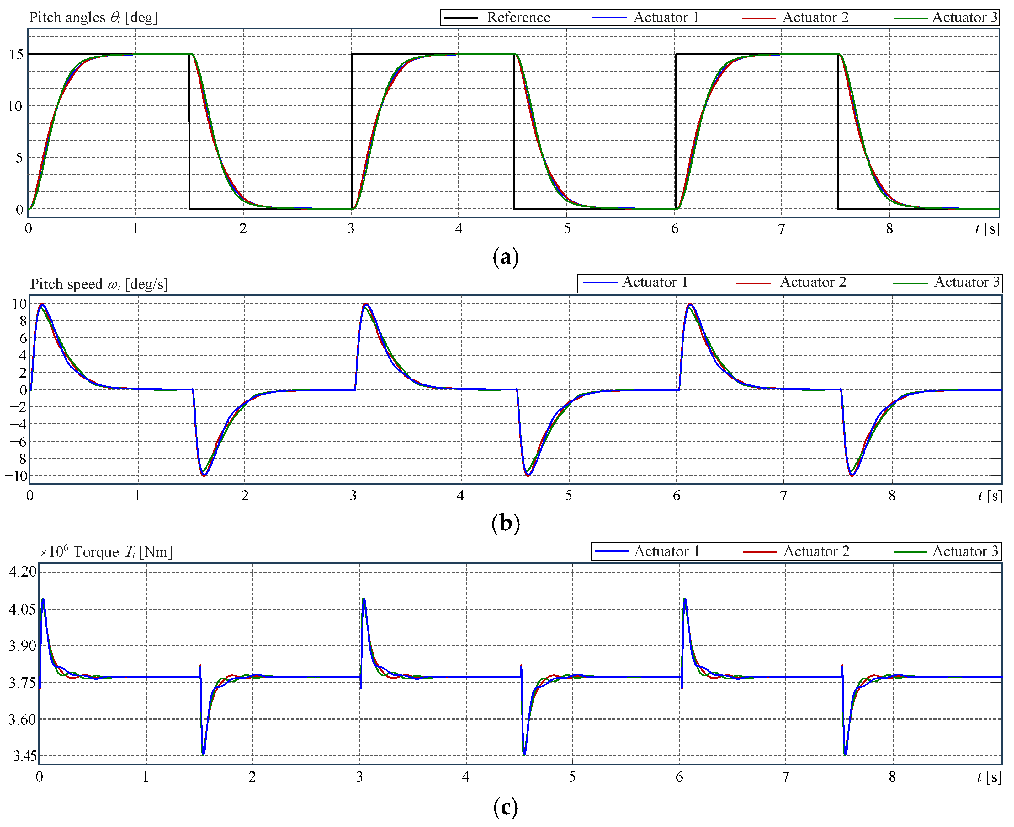
Figure 18. Simulation results for the first example. (a) Position angles. (b) Speeds. (c) Torques.

Figure 18a shows the resulting pitch angle of the blade (magenta curve) contrasted with the individual position angles of each actuator scaled by the gear rim ratio. Figure 18b shows the actuators and blade speeds, similar to how Figure 18a shows the angles. Figure 18c shows the synchronised torques entering the gear rim. As can be observed, the blade angle and speed closely match the individual actuator values, although they are not strictly considered in the synchronisation.

4.4. Example 2: Pitch Actuator Control on Three Different Blades

This example illustrates the other case presented in the introduction, namely, when the actuators have to satisfy a unique command from the CPC and all three blades are pitched simultaneously at the same angle. Because the three blades are independent, the relevance here is to synchronise the pitch angles of different blades. Contrary to the previous example, torques are not in the foreground. In order to obtain the required torque, three pitch actuators are attached to the same gear rim, as shown in the previous example. The configuration is presented in Figure 19.

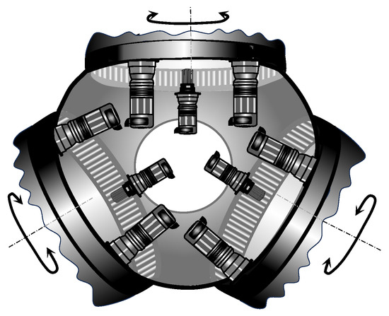
Figure 19. Three pitch actuators attached to each gear rim.

In order to simplify the simulation block diagram, all three actuators attached to one blade are represented now by a unique block. The simulation block diagram is presented in Figure 20.

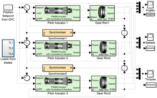
Figure 20. Simulation block diagram for the second example.

The control law of the synchronisers is also selected as for the previous examples. However, the optimal parameters of the PI controllers are, in this case, K_ps = 2.5022 and K_is = 0.3099. The simulation results are shown in Figure 21.

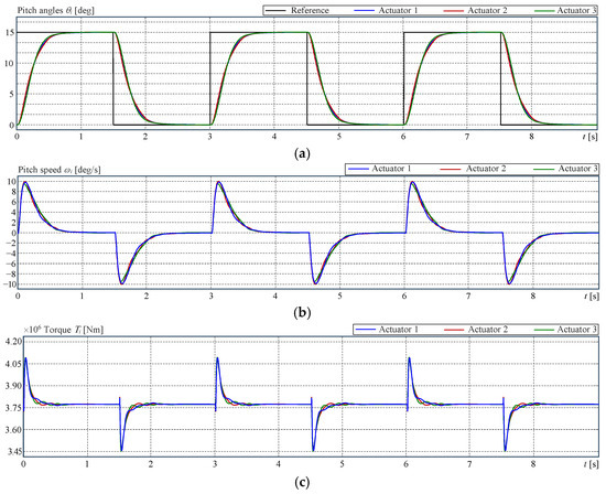
Figure 21. Simulation results of the second example. (a) Positions. (b) Speeds. (c) Torques.

The synchronised pitch angles are displayed in Figure 21a, where an improvement in collective pitch control is clearly appreciated. Moreover, Figure 18b,c show speeds and torques, respectively. Although the objective is to synchronise the pitch angles, speeds and torques are also synchronised, albeit to a diminished level.

5. Quantitative Evaluation of the Results

5.1. Context Description for the Assessment of Example 1

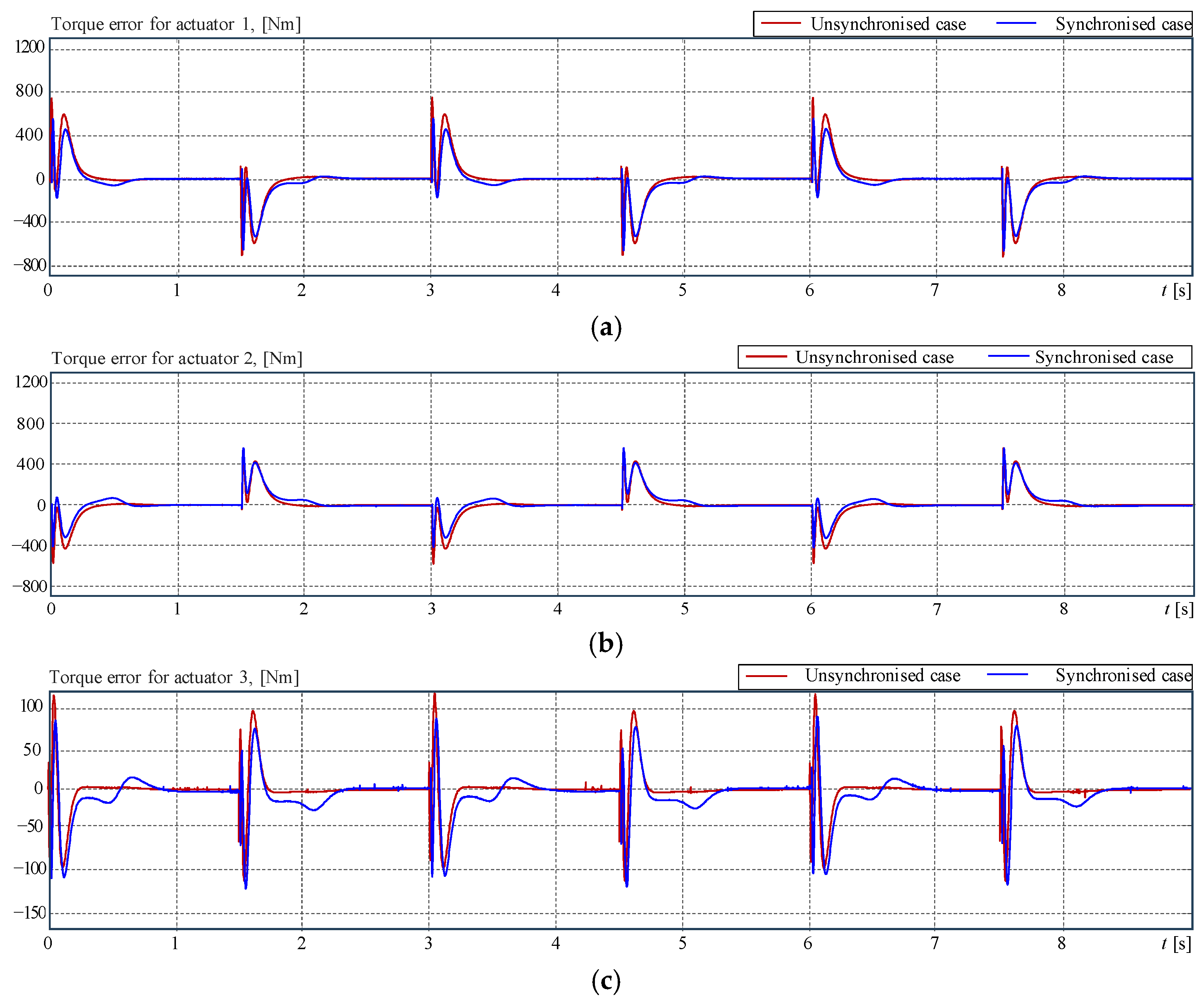
The objective of the first application example is to synchronise the torques coming from the pitch actuators in order to avoid disbalances on the gear rim. In the ideal case, all actuators provide the same torque, such that the torque acting on the blade is n_a times the torque of one actuator, where n_a is the number of actuators. Hence, the reference for the performance analysis is the average torque considering all contributors, i.e.,

$$T_{ref}(t)=(1/n_a){\displaystyle \sum _{i=1}^{n_a}{T}_{e,i}(t)}.$$

(68)

The performance is then evaluated by quantifying the deviation of each individual actuator torque from this reference. For this purpose, the performance index

$$J_{e,i}(s)={\displaystyle \frac{1}{t_f-t_0}}{\displaystyle {\int }_{t_0}^{t_f}{\left(\frac{e_i(t)}{e_{i,\max }}\right)}^2\hspace{0.17em}}dt$$

(69)

is defined, where, for the present case, e_i(t) = T_ref(t) − T_e,i(t), with i = 1…n_a. Hence, the index is computed for both unsynchronised and synchronised control, and the lowest value exhibits the best performance. This implies that the best result is when the torque of each actuator is closer to the average torque. The errors used for the performance evaluation are described in Figure 22.

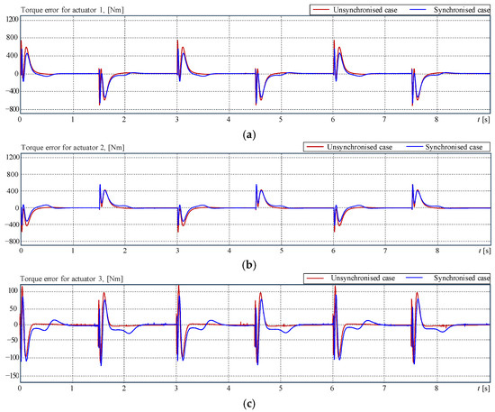
Figure 22. Errors between torques. (a) Actuator 1. (b) Actuator 2. (c) Actuator 3.

5.2. Context Description for the Assessment of Example 2

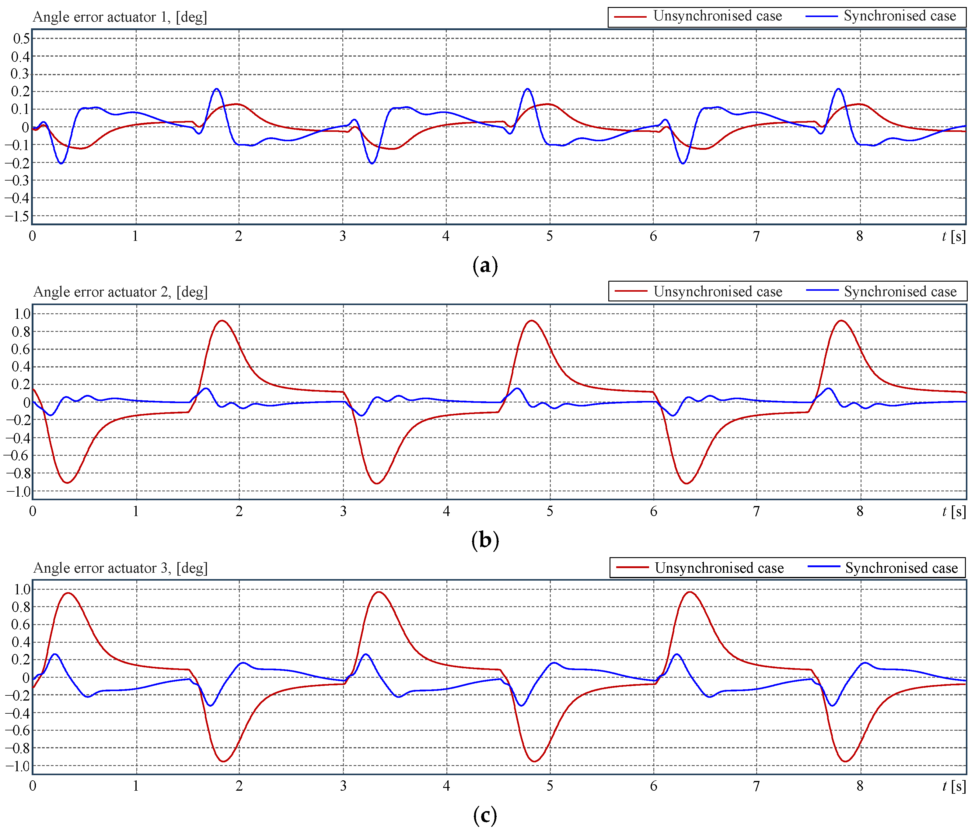
In the second example, the goal is to synchronise the pitch angles of the three independent blades. The evaluation process is similar to the previous one. The reference signal for the evaluation is the angle average of all actuators. The errors used in the performance index (69) are e_i(t) = θ_ref(t) − θ_i(t), for i = 1, 2, 3. The errors obtained by simulation are portrayed in Figure 23.

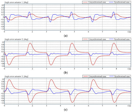
Figure 23. Errors between angles. (a) Actuator 1. (b) Actuator 2. (c) Actuator 3.

5.3. Concluding Remarks on the Quantitative Study

The error data presented in the previous sections are now used to obtain values of the performance index (69). The results are summarised in Table 3.

Table 3. Values of the performance index for all cases.

	Example 1 (Torque Synchronisation)			Example 2 (Angle Synchronisation)
	Actuator 1	Actuator 2	Actuator 3	Actuator 1	Actuator 2	Actuator 3
Unsynchronised control	1.485	1.362	1.365	1.003	6.328	7.151
Synchronised control	1.419	1.137	1.244	0.940	0.590	1.622

The first point that is immediately apparent is the close proximity of the values for the unsynchronised and synchronised cases of actuator 1. This is due to the fact that actuator 1 is the one designed according to the specifications, while the other two are obtained by parametric variation. For this reason, its errors are very close to the averages. On the other hand, it often happens that the synchronised error of this actuator is slightly poorer than the non-synchronised one, as a consequence of a strong adjustment to bring the other actuators closer to the average, which leads to a compromise.

In general, both examples show that synchronised control improves the overall closed-loop behaviour. However, it is also observable that angle synchronisation is better than torque synchronisation. This is so because torque synchronisation takes place indirectly through position control. In order to improve this result, a torque control loop is necessary. However, this is normally not possible to implement because the configuration of the internal actuator control system is fixed.

6. Conclusions

In this work, the problem of synchronising actuators of large wind turbines has been studied, and a synchronisation approach has been developed and successfully implemented in a simulation environment. The process started by modelling the actuator followed by the control system design, which has been verified using a well-known example from the literature. The focus was set on showing the effectiveness of a classic control methodology but with the improvement of considering a nonlinear gain for position control. Next, the typical synchronisation procedure of the control literature is extended to include the specific characteristics of the actuators. For the implementation of the examples, the pitch actuators have been parametrised for a 20 MW wind energy converter.

The presented examples represent real open aspects in the control of wind turbines, in particular in the case of actuator control. The results are very satisfactory and promising. The first example refers to indirect torque synchronisation in the pitch control of a single blade with multiple actuators. Improvements over and above those obtained so far will require modifying the internal topology of the actuator control system to include a torque control loop. However, this is a challenging problem because the idea is to include the torque control loop without increasing the already existing high complexity. A concept for this purpose is currently under study. The second example illustrates with excellent results the pitch angle synchronisation of three different rotor blades.

The obtained results are very satisfactory and promising. However, two additional aspects are now being considered. The first one is a sensitivity analysis against parameter uncertainty, as well as parameter drift. The second aspect involves assuming that the load torque may experience strong disturbances (extreme loads). Both cases will be considered in a new simulation study.

Another synchronisation problem in wind turbine control is caused by the control of the yaw motion. This instance is also a case of torque synchronisation, but the challenge is posed by the high number of actuators involved (between eight and sixteen, depending on the size of the wind turbine). Synchronised yaw control is the next investigative step.

References

- Bonfiglioli. Wind Solutions: Product Range. Product Description; Bonfiglioli Riduttori S.p.A.: Bologna, Italy, 2020. [Google Scholar]
- Gambier, A. Pitch control of three bladed large wind energy converters—A Review. Energies 2021, 14, 8083. [Google Scholar] [CrossRef]
- Hu, S.; Ren, X.; Zhao, W. Synchronous control of multi-motor driving servo systems. In Lecture Notes in Electrical Engineering 459; Jia, Y., Du, J., Zhang, W., Eds.; Springer: Singapore, 2017; pp. 611–620. [Google Scholar] [CrossRef]
- Li, M.; Meng, X. Analysis and design of system for multi-motor synchronous control. In Advances in Computer Science, Environment, Ecoinformatics, and Education 217; Lin, S., Huang, X., Eds.; Springer: Berlin/Heidelberg, Germany, 2011; pp. 268–273. [Google Scholar] [CrossRef]
- Niu, F.; Sun, K.; Huang, S.; Hu, Y.; Liang, D. A review on multimotor synchronous control methods. IEEE Trans. Transp. Electrif. 2023, 9, 22–33. [Google Scholar] [CrossRef]
- Unbehauen, H.; Vakilzadeh, I. Automatic error elimination between outputs of n identical simple integral plants with different initial conditions. Int. J. Control 1988, 47, 1101–1116. [Google Scholar] [CrossRef]
- Unbehauen, H.; Vakilzadeh, I. Feedforward technique in rendezvous problems for n identical simple-integral plants. Int. J. Syst. Sci. 1992, 23, 2091–2111. [Google Scholar] [CrossRef]
- Vakilzadeh, I.; Unbehauen, H. Tracking performance of ‘n’ integral-plus-time constant plants with ‘one’ controller. Kybernetika 1993, 29, 351–378. [Google Scholar]
- Unbehauen, H.; Vakilzadeh, I. Centralized control of n identical plants. J. Dyn. Syst. Meas. Control 1993, 115, 325–333. [Google Scholar] [CrossRef]
- Unbehauen, H.; Vakilzadeh, I. Synchronization of n non-identical simple-integral plants. Int. J. Control 1989, 50, 543–574. [Google Scholar] [CrossRef]
- Vakilzadeh, I.; Mansour, M. Synchronization of ‘n’ integral-plus-times constant plants with non-identical gain and time constants. Control Theory Adv. Technol. 1989, 5, 569–585. [Google Scholar] [CrossRef]
- Vakilzadeh, I.; Mansour, M. Synchronization of ‘n” integral-plus-double time constant plants with non-identical gain and time constants. J. FrankIm Inst. 1990, 327, 579–593. [Google Scholar] [CrossRef]
- Unbehauen, H.; Vakilzadeh, I. Synchronization of ‘n’ decentralized non-identical plants with integral behavior and two complex poles. Control Theory Adv. Technol. 1994, 10, 385–402. [Google Scholar]
- Vakilzadeh, I.; Unbehauen, H. Four rendezvous problems for n non-identical simple-integral plants. Int. J. Syst. Sci. 1993, 24, 1455–1472. [Google Scholar] [CrossRef]
- Koren, Y. Cross-coupled biaxial computer control for manufacturing systems. J. Dyn. Syst. Meas. Control 1980, 102, 265–271. [Google Scholar] [CrossRef]
- Zhao, D.; Li, C.; Ren, J. Speed synchronization of multiple induction motors with adjacent cross coupling control. In Proceedings of the 48h IEEE Conference on Decision and Control (CDC), Shanghai, China, 15–18 December 2009; pp. 6805–6810. [Google Scholar] [CrossRef]
- Gambier, A. Control of Large Wind Energy Systems; Springer Nature: Basel, Switzerland, 2022. [Google Scholar]
- Bianchi, F.D.; de Battista, H.; Mantz, R.J. Wind Turbine Control Systems; Springer: London, UK, 2007. [Google Scholar]
- Geng, H.; Yang, G. Output power control for variable-speed variable-pitch wind generation systems. IEEE Trans. Energy Convers. 2010, 25, 494–503. [Google Scholar] [CrossRef]
- Fortmann, J. Modeling of Wind Turbines with Doubly Fed Generator System; Springer Vieweg: Wiesbaden, Germany, 2014. [Google Scholar]
- Odgaard, P.F.; Stoustrup, J.; Kinnaert, M. Fault-tolerant control of wind turbines: A benchmark model. IEEE Trans. Control Syst. Technol. 2013, 21, 1168–1182. [Google Scholar] [CrossRef]
- Esbensen, T.; Sloth, C. Fault Diagnosis and Fault-Tolerant Control of Wind Turbines; Aalborg University: Aalborg, Denmark, 2009. [Google Scholar]
- Sloth, C.; Esbensen, T.; Stoustrup, J. Active and passive fault-tolerant LPV control of wind turbines. In Proceedings of the 2010 American Control Conference, Baltimore, MD, USA, 30 June–2 July 2010; pp. 4640–4646. [Google Scholar] [CrossRef]
- Krishnan, R. Electric Motor Drives: Modeling, Analysis & Control; Prentice Hall: Upper Saddle River, NJ, USA, 2006. [Google Scholar]
- Ong, C.-M. Dynamic Simulation of Electric Machinery; Prentice Hall: Upper Saddle River, NJ, USA, 1998. [Google Scholar]
- Park, R.H. Two reaction theory of synchronous machines. AIEE Trans. 1929, 48, 716–730. [Google Scholar] [CrossRef]
- Mohan, N. Advanced Electric Drives: Analysis, Control, and Modeling Using MATLAB/Simulink; John Wiley & Sons, Inc.: Hoboken, NJ, USA, 2014. [Google Scholar]
- Wang, L.; Chai, S.; Yoo, D.; Gan, L.; Ng, K. PID and Predictive Control of Electrical Drives and Power Converters Using MATLAB®/Simulink®; John Wiley & Sons: Singapore, 2015. [Google Scholar]
- Wach, P. Dynamics and Control of Electrical Drives; Springer: Berlin/Heidelberg, Germany, 2011. [Google Scholar]
- Vukosavić, S.N. Digital Control of Electrical Drives; Springer Science + Business Media, LLC.: New York, NY, USA, 2007. [Google Scholar]
- Melkebeek, J.A. Electrical Machines and Drives: Fundamentals and Advanced Modelling; Springer Nature: Cham, Switzerland, 2018. [Google Scholar]
- Krishnan, R. Permanent Magnet Synchronous and Brushless DC Motor Drives; CRC Press: Boca Raton, FL, USA, 2017. [Google Scholar]
- Carpiuc, S.; Villegas, C. Real–time position control in permanent magnet synchronous machine drives. In Proceedings of the 2018 20th European Conference on Power Electronics and Applications, Riga, Latvia, 17–21 September 2018; pp. P.1–P.8. [Google Scholar]
- Leonhard, W. Control of Electrical Drives, 3rd ed.; Springer: Heidelberg, Germany, 2001. [Google Scholar]
- Saafan, M.M.; Haikal, A.Y.; Saraya, S.F.; Areed, F.F.G. Artificial neural network control of permanent magnet synchronous motors. Int. J. Comput. Appl. 2012, 37, 9–18. [Google Scholar] [CrossRef]
- Wang, C.; Liu, B.; Fan, X.; Yang, P. Rotor position angle control of permanent magnet synchronous motor based on slidingmode extended state observer. Syst. Sci. Control Eng. Open Access J. 2022, 10, 757–766. [Google Scholar] [CrossRef]
- Carpiuc, S. Model–based control and real–time simulation of a four–phase PMSM traction drive. In Proceedings of the 2022 International Conference on Electrical Machines (ICEM), Valencia, Spain, 5–8 September 2022; pp. 2378–2383. [Google Scholar] [CrossRef]
- Kung, Y.-S.; Huang, P.-G. High performance position controller for PMSM drives based on TMS320F2812 DSP. In Proceedings of the IEEE International Conference on Control Applications, Taipei, Taiwan, 2–4 September 2004; pp. 290–295. [Google Scholar] [CrossRef]
- Ko, J.-S.; Han, B.-M. Precision position control of PMSM using neural network disturbance observer and parameter compensator. In Proceedings of the 2005 IEEE 36th Power Electronics Specialists Conference, Dresden, Germany, 16 June 2005; pp. 1313–1319. [Google Scholar] [CrossRef]
- Aguilar-Mejia, O.; Popocatl, H.M.; Garcia-Morales, J.M.; Castillo-Ibarra, C.O.; Valderrabano-Gonzalez, A. An efficient neurocontroller position method for PMSM drive system. In Proceedings of the 2022 IEEE International Autumn Meeting on Power, Electronics and Computing (ROPEC), Ixtapa, Mexico, 9–11 January 2022; pp. 1–6. [Google Scholar] [CrossRef]
- Liu, Q.; Chang, X.-H. Position IP control of a permanent magnet synchronous motor based on fuzzy neural network. In Proceedings of the 2018 Chinese Control And Decision Conference (CCDC), Shenyang, China, 9–11 June 2018; pp. 1081–1086. [Google Scholar] [CrossRef]
- Fertik, H.A.; Ross, C.W. Direct digital control algorithm with anti-windup feature. ISA Trans. 1967, 6, 317–328. [Google Scholar]
- Visioli, A. Practical PID Control; Springer: London, UK, 2006. [Google Scholar]
- Rundqwist, L. Anti-Reset Windup for PID Controllers. Ph.D. Thesis, Lund Institute of Technology, Lund, Sweden, 1991. [Google Scholar]
- Mohan, N. Power Electronics: A First Course; John Wiley & Sons, Inc.: Hoboken, NJ, USA, 2012. [Google Scholar]
- Bose, B.K. Power Electronics and Motor Drives: Advances and Trends; Elsevier Inc.: Burlington, VT, USA, 2006. [Google Scholar]
- Pyrhönen, J.; Hrabovcová, V.; Semken, R.S. Electrical Machine Drives Control: An Introduction; John Wiley & Sons, Ltd.: Chichester, UK, 2016. [Google Scholar]
- Johnson, M.A.; Moradi, M.H. PID Control—New Identification and Design Methods; Springer: London, UK, 2005. [Google Scholar]
- Gürocak, H. Industrial Motion Control: Motor Selection, Drivers, Controller Tuning, Applications; John Wiley & Sons Ltd.: Chichester, UK, 2016. [Google Scholar]
- Åström, K.J.; Murray, R.M. Feedback Systems: An Introduction for Scientists and Engineers; Princeton University Press: Princeton, NJ, USA, 2008. [Google Scholar]
- Gambier, A.; Nazaruddin, Y. Collective pitch control with active tower damping of a wind turbine by using a nonlinear PID approach. IFAC–Pap. 2018, 51, 238–243. [Google Scholar] [CrossRef]
- Shahruz, S.M.; Schwartz, A.L. Design of optimal nonlinear PI compensators. In Proceedings of the IEEE Conference on Decision and Control, San Antonio, TX, USA, 15–17 December 1993; pp. 3564–3565. [Google Scholar] [CrossRef]
- Xu, Y.; Hollerbach, J.M.; Ma, D. A nonlinear PD controller for force and contact transient control. IEEE Control Syst. Mag. 1995, 15, 15–21. [Google Scholar] [CrossRef]
- Gambier, A.; Jipp, M. Multi-objective optimal control: An introduction. In Proceedings of the Asian Control Conference, Kaohsiung, Taiwan, 15–18 May 2011; pp. 1084–1089. [Google Scholar]
- Ashuri, T.; Zaaijer, M.B.; Martins, J.R.R.A.; Zhang, J. Multidisciplinary design optimization of large wind turbines—Technical, economic, and design challenges. Energy Convers. Manag. 2016, 123, 56–70. [Google Scholar] [CrossRef]
- Gambier, A. Multiobjective optimal control of wind turbines: A survey on methods and recommendations for the implementation. Energies 2022, 15, 567. [Google Scholar] [CrossRef]
Disclaimer/Publisher’s Note: The statements, opinions and data contained in all publications are solely those of the individual author(s) and contributor(s) and not of MDPI and/or the editor(s). MDPI and/or the editor(s) disclaim responsibility for any injury to people or property resulting from any ideas, methods, instructions or products referred to in the content. |
© 2025 by the author. Licensee MDPI, Basel, Switzerland. This article is an open access article distributed under the terms and conditions of the Creative Commons Attribution (CC BY) license (https://creativecommons.org/licenses/by/4.0/).