Development of Real-Time Models of Electromechanical Actuators for a Hybrid Iron Bird of a Regional Aircraft

Abstract

This study presents the development of a real-time simulation model for electromechanical actuators tailored to a hybrid iron bird for next-generation regional turboprop aircraft. This iron bird is aimed at integrating real and virtual components, enabling advanced validation of flight control systems while balancing risk and cost. The mathematical models of actuators needed for the development and operation of the iron bird must comply with stringent requirements, especially in terms of computational cost. A novel two-step iterative methodology is proposed, combining bottom-up and top-down approaches. This process begins with simplified low-fidelity models. Then, the models are incrementally refined to capture complex dynamics while maintaining computational efficiency. Using the proposed approach, the computational time of the real-time model remained almost unvaried and consistent with the sampling frequency, while the number of state variables and the range of described phenomena grew significantly. The real-time model is validated against simulated data from a reference high-fidelity model and experimental data, achieving excellent agreement while reducing the computational time by 93%. The enhanced model incorporates selected failure modes equivalent models regarding the electric motor, power drive unit, and mechanical transmission, supporting possible future prognostics and health management (PHM) applications. These results showcase a scalable solution for integrating electromechanical actuation in modern aerospace systems, paving the way for full virtual iron birds and greener aviation technologies.

1. Introduction

This work proposes an incremental approach for the real-time model development of electromechanical actuators. The approach is driven by multiple verification/validation needs and by the software and hardware constraints relative to the real-time simulator realization.

This section introduces the global context of the real-time simulation of electromechanical actuators (EMA).

1.1. Need for Real-Time Models of Electromechanical Actuators

In addition to the need to develop more efficient operations and new services, decarbonization of air transport raises a huge challenge to put innovative and mature solutions to market [1]. High-power actuators for flight controls or landing gears are directly concerned because they are key enablers toward greener, safer, and cheaper aerospace. The most recent single-aisle and long-range models proposed by the key airframers have already benefited from the latest advances in fly-by-less-wire (FblW) and power-by-wire (PbW): e-rudder for the Airbus A320, electro-hydrostatic actuators (EHA) for the Airbus A380/350, and EMAs for a few spoilers on the Boeing 787 [2]. Apart from them, regional aircraft have not yet taken such benefits. There is, therefore, a huge interest in improving their performance through the introduction of more electrical actuation for advanced flight controls, providing better aerodynamics, reduced air loads, and efficient health monitoring features.

In this context of innovation, the extensive use of models and digital simulation of actuators provides potentially an efficient means to reduce risks and costs toward entry into service. Off-line simulation is now well established for each phase of life, from equipment to aircraft levels: architecting, design, integration, verification and validation, training, and maintenance. For actuation, it involves system-level multiphysics simulation [3,4], which is facilitated by the wide offer of dedicated model libraries that are available in several commercial simulation software packages. They enable the users to make, at a low coding effort, very detailed models of actuators, involving hundreds of parameters and state or algebraic variables.

Aircraft-level integration tests aim at simulating on ground the correct operation of all safety-critical systems during a flight when they are interconnected, in nominal or degraded conditions. This is performed on the general integration test rig, which is commonly known as the iron bird or aircraft-0 [5,6,7]. In the conventional approach, the aircraft flight mechanics is simulated in real time (RT): the evolution of the simulated time is synchronized to real time. The RT simulation computes the air load setpoints for the actuators [8], which are used to load the aircraft flight controls or landing gear real actuators. On their side, the fly-deck, flight control computers, power networks, and actuators remain real. Their interconnection and topology are kept as close as possible to those of the real aircraft. In recent years, heavy data transmission and fast processing have progressed incredibly, paving the way toward full virtual iron birds. RT simulation of conventional hydraulically supplied actuators has become well-established [9]. Oppositely, the RT simulation of EMAs is still more challenging when it is intended to get realistic simulations for virtual validation. This comes mainly from the specificity of EMAs, involving, for example, fast switching at electronics, backlash and friction at mechanical reducers, issues with thermal balance, and risk of jamming. This makes virtual testing harder, in particular for the validation of the advanced flight control laws, the sizing of electric power generation and distribution networks, and the health-monitoring strategies [10].

Additionally, any advance to make the virtual tests more realistic contributes to increasing the admittance of the regulatory authorities to the use of virtual tests for certification of safety-critical applications like flight controls [11].

The present work reports the activity performed toward this target for the new generation of regional turboprop aircraft. It relates to the advances made to develop such real-time simulation models of EMAs in order to get the Permit to Fly through onground, fully simulated flight. Section 1 gives an introduction to the project scope and the EMA’s architecture and modeling; Section 2 deals with the analysis of the real-time modeling constraints in modeling EMA’s dynamics; Section 3 is dedicated to the implementation of the real-time model and describes the adopted development process as well as the starting reference simple model; Section 4 explains the computational cost reduction techniques exploited in this work and their application in the reference model; Section 5 describes the additional phenomena that were added to the initial reference model to enhance its descriptive capabilities in terms of output response fidelity and accuracy; Section 6 shows the results of the work in terms of model’s computational time reduction effectiveness and response validation against reference experimental and simulated data; and finally, Section 7 presents the conclusions.

1.2. Hardware-in-the-Loop Testing

In the model-based approach, the activities ideally start by using virtual objects that are built from models and their numerical simulation and interfacing. As the project progresses, the verification and validation tasks are performed by progressive integration and replacement of virtual objects, e.g., an electromechanical actuator with the real ones that will be used in the final product. Combining simulated and real objects can be achieved in different ways given the current task to be performed. Although the acronyms are not standardized, the following are commonly used:

• In hardware-in-the-loop (HIL) testing, hardware (or a part of it) is virtual. A distinction can be made whether the virtual hardware is modeled with a power view (pHIL), a signal or computer view (sHIL of cHIL), or even a mechanical view (mHIL) [12,13,14].
• In rapid control prototyping (RCP) tests, the real controller is replaced by a simulated one, while the controlled object remains real.
• Combining HIL and RCP leads to software-in-the-loop (SIL) testing where the engineered software code is implemented on a substitute of the product processor, and the controlled object is also simulated.

All these “-In-the-Loop” tests usually require real-time simulation of the models to accurately evaluate how time-related factors affect the system and its integration, including dynamics, delays, computational load, interactions between components, and so forth.

1.3. Electromechanical Actuators and Their Real-Time Simulation

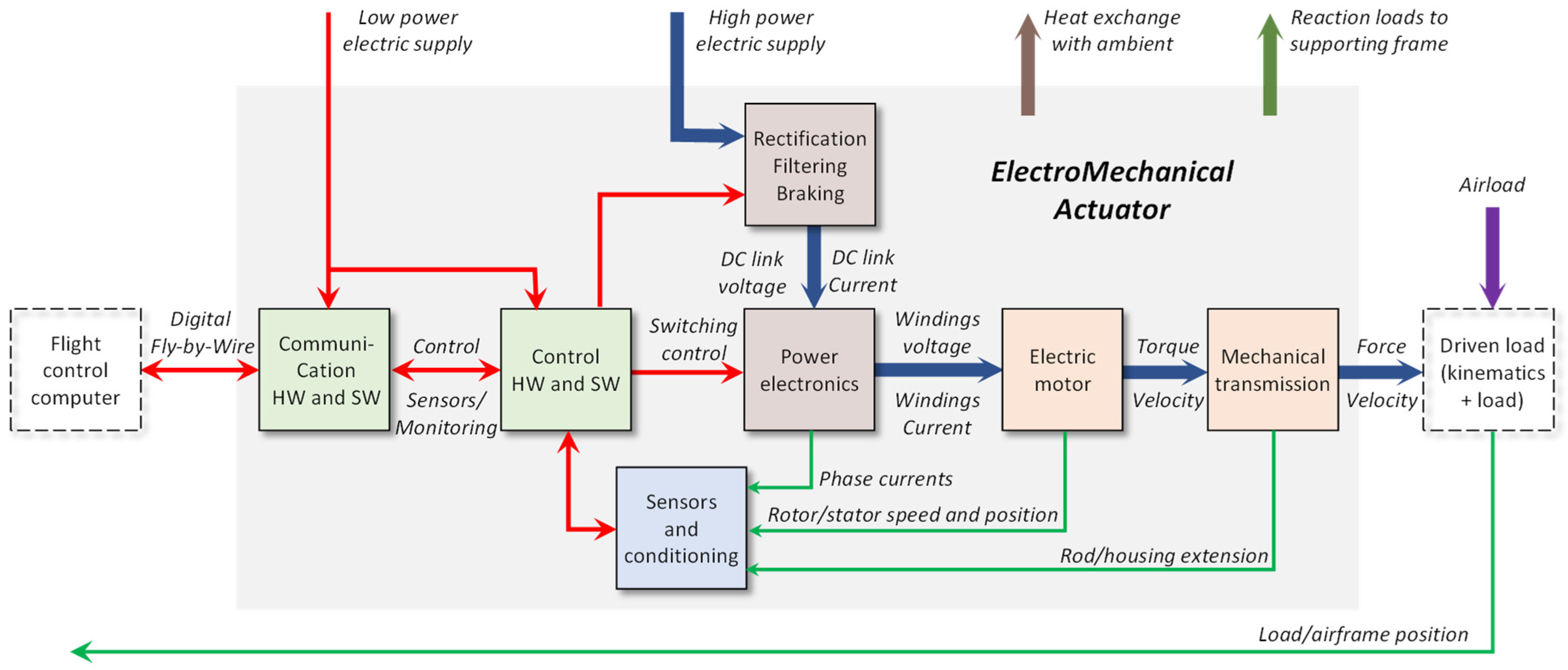
Figure 1 displays the generic elements of a digitally signaled linear electromechanical actuator. It also highlights the actuator interfaces. The main power-level elements are:

• If needed, a DC link, which makes a constant DC source from the 3-phase AC supply;
• An inverter, which acts functionally as a variable power transformer between the DC source and the motor windings, which are controlled by the modulation ratio demand;
• A motor, generally a permanent magnet synchronous machine (PMSM), which acts functionally as a power transformer between the electric and rotational mechanical domains;
• A mechanical transmission, including a nut/screw system, which acts functionally as a power transformer between the rotational and translational mechanical domains. For geared EMA designs, an intermediate gear reducer acts functionally as a power transformer between the high-speed/low-torque and low-speed/high-torque rotational mechanical domains.

The main signal-level elements are:

• The actuator sensors (measuring, for example, the windings currents, motor rotor speed/angle, and rod extension) with their supply and conditioning;
• A controller in charge of driving the inverter and performing the actuator position control, generally with inner rotor speed and current loops;
• Data bus interfaces to enable communication to/from the flight control computers.

Although they are not the responsibility of the actuator supplier, the anchorage of the actuator body to the supporting frame, the kinematics to the actuated load, and the load itself can also be considered part of the actuation function to simulate [15].

Table 1 presents a synthetic review of the bibliography addressing real-time simulation of actuation systems and electric drives. The different levels of RT simulation clearly appear, from the piloting of a real loading system [8,16] to the full system simulation. Four main uses and applications can be identified:

• Full system assessment, for example for electric car drives [17], aircraft pitch control [18], or flight simulation [19];
• Health monitoring and protections, for example, in case of motor winding short circuits [20,21], to implement protections [22] or suppression [23];
• Assessment of control design, for example, sensorless control [24] or sliding mode control [25];
• Pure improvement of real-time models of electric machines, for example [26,27,28].

It is important to note that many references use the real-time model in the final product itself, for example, to implement advanced control laws [24] or thermal protection [22].

Table 1 clearly shows that most of the references focus on two main topics:

• The modeling of the power electronics and electric motor, without any, or with very simplified, considerations of the mechanical part (which is functionally downstream of the electromagnetic power transformation);
• Architecture, software, and hardware used to implement real-time simulation in the presence of very high dynamics at inverter and motor, with very few details on the models used.

It is worth mentioning that no reference addresses, even partly, the measurement and acquisition chains, in particular concerning their influence on performance and the constraints that they impose on the real-time simulation.

Table 1. References related to real-time simulation for electromechanical actuation.

Ref	Purpose and Contribution					Power Elements Modeled				Implementation
	Type	Controller Assessment	Health Monitoring Protection	Improvement of RT Model	Full System Assessment	Inverter	Motor	Mechanical Transmission	Load
[22]	HIL		Thermal protection			No	7-bodies thermal model Analytical h coefficients from generic geometry	No	No	CPU
[26]	HIL			Numerical stability		No	dq0 model, spatial inductances	No	No	CPU
[23]	SIL		Supervision of e-car				Common models for copper and iron losses	Bond graph only	Bond graph only	?
[24]	HIL				Sensorless control		3-phase Current-dependent inductances	Yes *	Yes *	FPGA and CPU
[29]	HIL				CPU/FPGA		3-phase constant parameters	Constant load + pure inertia + viscous friction		FPGA and CPU
[25]	SIL	Sliding mode control				Yes *	Basic equivalent DC	Yes *	No load	CPU
[21]	HIL		Fault models			Yes *	4D tables for inductances from FEM (turn-to-turn short circuits)	Perfect	Constant motor load	FPGA
[16]	HIL	Sizing and control				No	No	Real loading motor to apply the RT-calculated load torque		CPU
[17]	?				Compared machines	Yes *	Motor inductance vs. current Motor resistance vs. rotor angle Flux linkage vs. current and rotor angle	Perfect	Rolling, air drag, gravity	FPGA
[27]	HIL			Motor model		No	(I, Q)-dependent parameters Magnetic saturation, iron core losses	No (steady state, imposed toque)	No	FPGA
[20]	SIL		Faults models			First-order equivalent * Short circuit modeled with shape function Hysteresis control		Second order * Rotor eccentricity modeled with shape function		?
[18]	SIL				Unified solver	With DC link *	4-bodies thermal model	Yes *	From aircraft *	FPGA
[19]	SIL				Flight simulation	No	Basic equivalent DC + constant cogging torque	Simplified Coulomb friction Backlash as an angular dead zone		?
[28]	SIL				Validation of RT implementation	?	5-phase 1st and 3rd harmonics of flux linkage	No	Pure inertial and viscous	FPGA and CPU

* Not detailed.

Table 1. References related to real-time simulation for electromechanical actuation.

Ref	Purpose and Contribution					Power Elements Modeled				Implementation
	Type	Controller Assessment	Health Monitoring Protection	Improvement of RT Model	Full System Assessment	Inverter	Motor	Mechanical Transmission	Load
[22]	HIL		Thermal protection			No	7-bodies thermal model Analytical h coefficients from generic geometry	No	No	CPU
[26]	HIL			Numerical stability		No	dq0 model, spatial inductances	No	No	CPU
[23]	SIL		Supervision of e-car				Common models for copper and iron losses	Bond graph only	Bond graph only	?
[24]	HIL				Sensorless control		3-phase Current-dependent inductances	Yes *	Yes *	FPGA and CPU
[29]	HIL				CPU/FPGA		3-phase constant parameters	Constant load + pure inertia + viscous friction		FPGA and CPU
[25]	SIL	Sliding mode control				Yes *	Basic equivalent DC	Yes *	No load	CPU
[21]	HIL		Fault models			Yes *	4D tables for inductances from FEM (turn-to-turn short circuits)	Perfect	Constant motor load	FPGA
[16]	HIL	Sizing and control				No	No	Real loading motor to apply the RT-calculated load torque		CPU
[17]	?				Compared machines	Yes *	Motor inductance vs. current Motor resistance vs. rotor angle Flux linkage vs. current and rotor angle	Perfect	Rolling, air drag, gravity	FPGA
[27]	HIL			Motor model		No	(I, Q)-dependent parameters Magnetic saturation, iron core losses	No (steady state, imposed toque)	No	FPGA
[20]	SIL		Faults models			First-order equivalent * Short circuit modeled with shape function Hysteresis control		Second order * Rotor eccentricity modeled with shape function		?
[18]	SIL				Unified solver	With DC link *	4-bodies thermal model	Yes *	From aircraft *	FPGA
[19]	SIL				Flight simulation	No	Basic equivalent DC + constant cogging torque	Simplified Coulomb friction Backlash as an angular dead zone		?
[28]	SIL				Validation of RT implementation	?	5-phase 1st and 3rd harmonics of flux linkage	No	Pure inertial and viscous	FPGA and CPU

* Not detailed.

2. Preliminary Considerations

This section provides preliminary considerations about engineering needs, the dynamics in presence, the RT simulation algorithms and the model reduction.

2.1. Engineering Needs for RT Models of Electromechanical Actuators

When used in aircraft-level integration and validation test rigs, various verification/validation tasks require the actuators to be RT simulated, such as:

• Sctuator/aircraft integration at signal levels, dealing mainly with the communication with the flight control computers, which is particularly important for digitally signaled flight controls;
• Actuator position control performance in the presence of realistic air loads computed from the simulation of the rigid or elastic aircraft flight mechanics, in particular regarding the risk of aero-servo-elasticity flutter;
• Robustness of control performance vs. operating conditions, at any point of operation, vs. accumulated service, ambient temperature, and supply voltage;
• Response to actuator faults, with a focus on detection, isolation, and reconfiguration;
• Overall energy consumption, mean and transient power draw from electric supplies, in normal and faulty conditions.

2.2. Dynamics in Presence

As a first step, it is important to summarize the orders of magnitude of the various dynamics that are present in EMAs, as illustrated in Figure 2. A second step consists of linking the project needs to the effects to be considered in the RT models. In such a way, combining these two steps enables the designer to specify or select the relevant hardware and simulation environment. At the aircraft level, it is not required to simulate in detail the switching of the inverter transistors and the motor parameters that depend on the actual winding currents and electric angle. In this case, there is no particular need to use FPGA, and a cheaper and more flexible CPU implementation is generally acceptable.

2.3. Real-Time Integration Algorithms

The techniques for real-time numerical integration are nowadays well established. More than half a century ago, low-order integration schemes (Euler, Adams–Bathforth, and Adams–Moulton methods) were already selected and combined for non-aerodynamic rigid-bodies space flight simulation [30]. More recently, the candidate techniques have been reviewed in [31], showing that low-order explicit methods are well suited to RT simulation as long as the model is not too discontinuous or numerically stiff. If this condition is not met, the author proposes alternatives involving linearly implicit methods, multi-rate, or mixed-mode integration. Unfortunately, the commercial off-the-shelf simulation environments offering automatic conversion of models into real-time software code only accept one solver type and order to be selected. This is confirmed in the references listed in Table 1, which use a single solver, for example, discrete [29], forward Euler [21,24], or even Runge–Kutta order 4 [18].

2.4. Model Reduction

There are two main ways to develop a RT model. The incremental approach consists of progressively increasing the realism and, therefore, the numerical complexity and computation burden from a simple, low-fidelity reference model. The decremental approach is the opposite: a very detailed and realistic model is progressively simplified to meet the engineering needs under the RT constraints. Several means can be used to assess the dynamics in the presence of a given high-fidelity model:

• Analysis of the calculation of the poles and zeros of a linear model. For power systems, the dynamics come from the combination of resistances, inertances, and capacitance effects that are modified by the presence of the different control loops;
• Simulation of the high-fidelity model, taking benefit of the numerical simulation environment features: spectrum analysis or numerical linearization from time responses, solver statistics/profilers, or activity indexes [32].

The simplification of lumped-parameter models can be achieved by resorting to well-established approaches. The most common ones are the model order reduction algorithm (MORA) and the singular perturbation method (SPM) [33]. However, they are difficult to apply when the intent is to keep an RT access and a physical meaning of some internal variables of interest, in particular for advanced control or health monitoring. These variables are, for example, the motor winding currents or voltages, the motor rotor speed, the actual gap in the backlash effect, or the heat-generated energy losses.

3. Development of the EMA RT Models for the Hybrid Iron Bird

This section provides details on the hybrid iron bird architecture, the RT simulator implementation, the RT model development, and the reference EMA model.

3.1. Desing of the Hybrid Iron Bird

The EMA RT models, the objective of the present paper, have been developed in the frame of the Astib CleanSky2 program, which aims to develop innovative aircraft demonstrator platforms (IADPs) for regional aircraft [34,35]. Being hybrid, the aircraft integration test rig, schematized in Figure 3, is itself innovative: it combines a real iron bird for the right wing and a virtual one for the left wing [7,36]. The real-time models of the actuators are implemented in the simulation module, while the flight mechanics is simulated in a dedicated simulation computer. Each simulated actuator model also outputs the power drawn by the actuator from the electrical DC source, which is used to command the piloted real electrical loads.

The hybrid iron bird design offers several advantages:

• It is an intermediate solution toward full virtual iron birds, which balances risks and effectiveness while facilitating experience feedback and reducing costs.
• It enables faults to be easily injected at (virtual) actuators level without any need to alter or risk damaging the real ones.
• Finally, it is an important enabler for the aircraft maker to take a huge step forward and obtain the Permit to Fly, introducing, at the same time, electromechanical actuation and digital fly-by-wire, air load alleviation for weight saving and increased passenger comfort, and morphing wing for more efficient aerodynamics.

3.2. Implementation of the EMAs RT Models

The EMAs RT models were developed in the Matlab-Simulink environment (R2024b). They were first tested on a SpeedGoat RT target computer (Intel Core 2 Duo 2.23 GHz CPU) with automatic translation from the MATLAB/Simulink models. For implementation in the simulation module of the IB, the models were translated to the National Instrument/Veristand environment and run on an Advantech AIMB-786G2 (4-core, 3.6 GHz, Intel Core i3-8100 CPU). Data interfacing with other real or simulated parts of the iron bird (about 1500 dynamic variables exchanged) was achieved at a 500 Hz frequency through an optical ring making a reflective memory. The RT integration fixed step was ≈0.083 ms (12 kHz) to properly describe the electrical dynamics while remaining within the real-time target capabilities. Advanced health monitoring features at actuator or aircraft levels were also assessed by running specific virtual tests that involved only two advanced RT models of the EMAs (81 parameters and 23 state variables).

The direct-drive, linear EMAs to be modeled have a constant DC voltage supply and use a 3-phase PMSM with sinusoidal back-EMF and inner rotor with surface-mounted permanent magnets and an electromechanical normally closed brake, Figure 4. This typology is coherent with the electric motors usually employed in aircraft control surface actuation.

The digital EMA controller is of common cascade type with rod position, motor rotor speed, and motor current loops. The inner motor current loop implements a vector control, forcing a 90° torque angle [37].

3.3. Process for the Development of the EMAs RT Models

The RT simulation has been addressed very early in the project to reduce risks and facilitate decision-making for the detailed specification of the hybrid iron bird. As high-fidelity models were not available in these early phases, the incremental approach was logically preferred. This choice was also motivated by the limited applicability of the common methods for model reduction, mentioned in Section 2.4. The RT model development started with a low-order reference model, which was progressively made more realistic while meeting the RT constraints. This was achieved by running a two-step loop several times:

• Step 1: a reduction of the RT computational burden to meet the real-time constraints through more efficient numerical implementation of the model;
• Step 2: increasing the model realism to extend the validation scope through the consideration of additional effects or more advanced modeling of already considered effects.

3.4. Reference Model

The structure of the reference model is representative of the architecture of the considered EMA and its driven load, as illustrated in Figure 5. The bond graph formalism is used for the power elements to make the graphical representation more compact. The causality marks indicate the model calculation structure, which does not involve any algebraic loops. This reference model is built by considering the following phenomena:

• Electronic actuator control unit (EACU): P-I continuous-time controllers with anti-windup function and output limitation;
• Power drive electronics: perfectly modulated transformer plus conduction losses (constant resistance R_c) and iron losses (constant percentage of motor current with nonlinear effect ➊);

• Electric motor: DC equivalent with constant parameters (resistance R_m and inductance L_m of windings and motor electromagnetic constant K_m);
• Nut/screw: power transformation with lead l, nonlinear friction model ➋ with Karnopp implementation for true sticking, and constant stiction and dynamic friction torques;
• Kinematics and surface: rigid 3-bar kinematics through trigonometric relations—nonlinear effect ➌, structural compliances lumped at EMA/kinematics interface level as a linear spring/damper (k_t, b_t), and surface moment of inertia J_s;
• Inertia of EMA moving bodies: single equivalent inertia J_e lumped at the translating nut level.

The dashed power bonds in Figure 5 indicate that the reference model calculates the heat generated by each energy loss. As no model parameter is yet temperature-sensitive, the ambient temperature is not used in the reference model, which is, therefore, isothermal. The models in dashed blocks are not included in the reference model for simplicity.

Finally, the model is of 8th order. Except for the three nonlinearities ➊➋➌, it is fully defined by Figure 5. In order to get a very preliminary view of the effective dynamics present,

Table 2. An early calculation of the time constants or periods of the dynamics present (time scale ratio referenced to the specified position loop dynamics).

Considered Effect	Time Scale Ratio
Motor housing thermal time constant	8797
Power drive unit thermal time constant	5278
Motor winding thermal time constant	88
Position closed loop (time constant or equivalent first order)	1
Time constant of P-I speed controller	0.601
Mechanical time constant at motor Je.Rm/Km2	0.327
Motor electric period at max speed	0.320
Sampling of position setpoint from FCC	0.220
Time constant of P-I current controller	0.123
Electric time constant of motor windings	0.096
Sampling period of the position control loop	0.088
Sampling period of the speed control loop	0.029
Period of cogging torque at max motor speed	0.027
Period of the excitation carrier for the rod LVDT position sensor	0.022
Sampling period of the current control loop	3.65 × 10−3
Sampling period of the duty cycle driving the inverter	7.35 × 10−6

was generated using formal calculations only, from the EMA design parameters. The dynamics are made dimensionless, with reference to the specified actuator dynamics (the equivalent time constant of the position loop). They are listed from the slower to the faster one. The table clearly shows the high numerical stiffness of the system, represented by the huge range of dynamics, with a +10⁹ ratio between the slowest and fastest ones.

4. Reduction of the Model Computational Time

Before increasing the fidelity of the above-mentioned reference modelby adding more and more physical phenomena, it is important to perform a preliminary check and verify the computational time required by the model to execute a single time step of the simulation, known as the task execution time (TET).

In fact, the TET is a key limiting parameter in real-time applications: it is paramount that the time required by the real-time target is sensibly slower than the maximum allowed time. Once the information exchange rate of the simulation module is decided, the TET must be lower or, at least, equal to this limit in order to not incur overruns. Actually, to remain conservative, the TET should not take more than approximately half the limit time because of the time allocation required by the operations of communication and reception of data by the other simulation architecture nodes. Furthermore, jitter in the TET is always present due to non-deterministic reasons connected and directly dependent on the RT hardware [38]: thus, it can be possible that random TET increases can cause an overrun error and the shutdown of the application.

Figure 6 depicts a typical situation of overrun during RT operations: it can be clearly seen that the error comes from having exceeded the maximum allowed fixed time. This situation must be avoided, and a certain safety margin should be considered. In particular, when the RT simulation is in parallel and in cooperation with real hardware components, the simulation abort due to overrun may cause serious damage to physical components. In fact, in such a case, the latter see the lack of data from the RT target as a consequence of some real behavior and may be commanded in such a way as to compensate or react to the anomalous situation, operating out of the design safety range.

Therefore, a trade-off analysis should be performed to find a balance between the need for increased model fidelity, with consequent increased computational effort, and the need to not excessively augment the calculation time in order to allow the correct operation of the RT target.

With this aim, several computational time reduction techniques have been tested and the most effective have been applied to the model described in the previous sections: they will be presented hereinafter together with the description of the updates of subsystems on which they have been used. It is worth mentioning that the following approach is not the only possible one; however, it aims to fully preserve the physics-based relationship within the model in order to allow a physical interpretation of the internal signals and results with the goal of applying PHM algorithms to meaningful data.

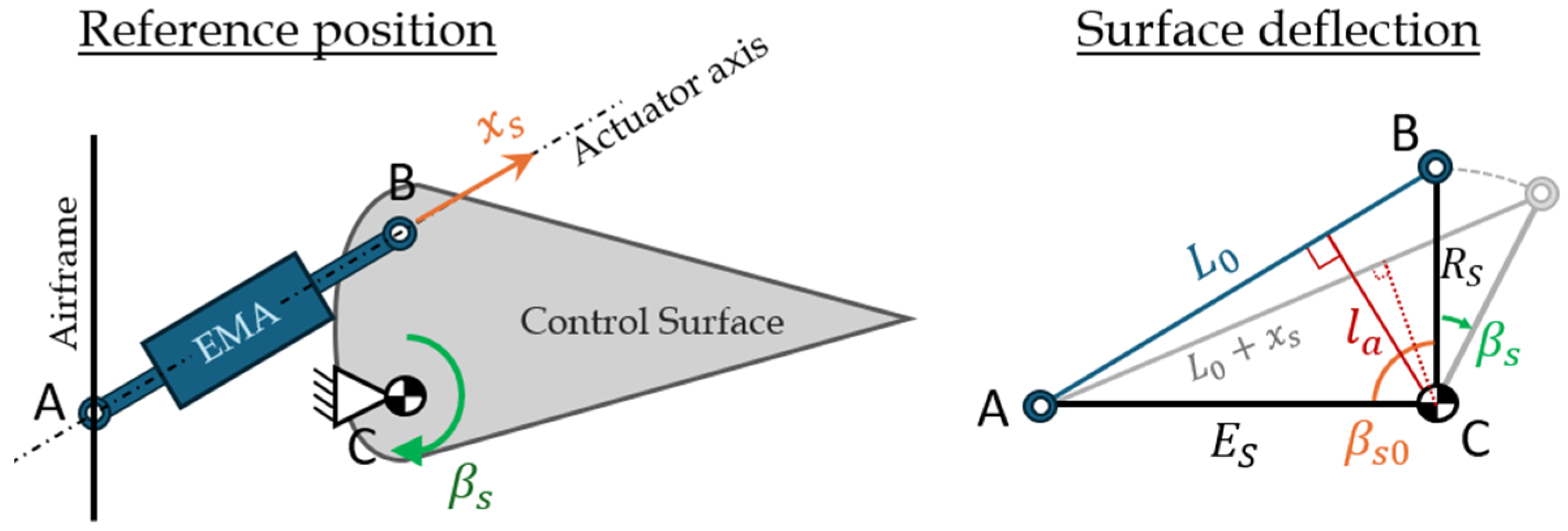
4.1. Simplification of Complex Mathematical Expressions—Rigid 3-Bar Kinematics

The first and most intuitive approach to reduce the computational time is to reduce the number and complexity of already present calculations, in particular for the nonlinear parts of the model. This technique has been applied to the surface subsystem, in particular, to simplify the modeling of the variable lever arm. As shown in Figure 7, the nonlinear variable power transformation made by the 3-bar kinematics links the EMA translational and surface rotational power variables with a position-dependent lever arm $l_a$.

Indicating with $x_s$ the EMA’s linear elongation with respect to the reference length $L_0$, as shown in Figure 7, the instantaneous relationship between the rotational and translational domains, in terms of kinematics, forces and torques, can be expressed as:

$$\left\{\begin{array}{c}{\dot{x}}_s=l_a\left({\beta }_s\right)·{\dot{\beta }}_s\\ T_s=l_a\left({\beta }_s\right)·F_r\end{array}\right.$$

(1)

In order to avoid any algebraic loop, the lever arm is calculated from the surface angular deflection ${\beta }_s$, leading to:

$$l_a\left({\beta }_s\right)=\sqrt{E_s^2-{\left({\displaystyle \frac{(E_s^2-R_s^2+{L_0}^2)}{2L_0}}\right)}^2}$$

(2)

with

$$L_0=\sqrt{E_s^2+R_s^2-2E_s{R}_s\cos ({\beta }_s+{\beta }_{s0})}$$

(3)

where $R_s$ is the distance of the EMA attachment B from the hinge point C, $E_s$ is the distance between the hinge C and the actuator attachment to the airframe A, and ${\beta }_{s0}$ is the surface deflection angle when $x_s=0$.

As previously stated, the rod end force $F_r$ is obtained from an elastic-damping connection model between the EMA and the control surface. The connection compliance is mainly linked to the rod end’s pin/bore contact stiffness, but to a certain extent, it can also be representative of the entire EMA structural elasticity. As such, the relationship between $x_s$ and ${\beta }_s$ is also needed to evaluate the elastic contribution. Considering that both $l_a$ and ${\beta }_s$ are time-dependent, the time derivative of the variable lever arm is also required, expressed as:

$$\begin{gathered} {\displaystyle \frac{d{l}_a\left(\beta \right)}{dt}}=-{\displaystyle \frac{E_s{R}_s\sin \left({\beta }_{s0}+{\beta }_s\right){\dot{\beta }}_s\left(\frac{{\sigma }_2}{{\sigma }_1}-\frac{{\sigma }_2^2}{2{\sigma }_1^2}\right)}{2\sqrt{E_s^2-\frac{{\sigma }_2^2}{4{\sigma }_1}}}} \\ {\sigma }_1=E_s^2+R_s^2-2E_s{R}_s\cos \left({\beta }_{s0}+{\beta }_s\right) \\ {\sigma }_2=2E_s^2-2E_s{R}_s\cos \left({\beta }_{s0}+{\beta }_s\right) \end{gathered}$$

(4)

From an RT perspective, this formal model of the 3-bar kinematics is not efficient:

• It does not explicitly provide the linear position and, depending on how the model is structured, can require an additional integration in the spring/damper model of rod/kinematics compliance.
• It involves a lot of mathematical calculations which puts a high penalty on the computational burden.

For these reasons, the lever arm $l_a\left({\beta }_{\mathrm{s}}\right)$ exact model of Equation (2) has been approximated with a polynomial representation model:

$$l_a^{^}\left({\beta }_s\right)=\sum _{i=1}^n{p}_i{\beta }_s^{n+1-i}$$

(5)

Consequently, the kinematic translational position at the surface level can be obtained integrating parts and considering the approximation of Equation (5):

$$x_s=\int \left[l_a\left({\beta }_s\right)·{\dot{\beta }}_s\right]dt=\sum _{i=1}^{n+1}{\displaystyle \frac{p_i{\beta }_s^i}{i}}$$

(6)

It is worth mentioning that the parameters of the polynomial representation models (Equations (5) and (6)) are not explicitly linked to the design parameters of the kinematics. However, this can be accepted for RT simulation when it is not intended to use the models for design exploration.

The model parameters $p_i$ have been identified off-line to minimize the root-mean-square modeling error ${\epsilon }_l=\sqrt{{\displaystyle \frac{1}{m}}{\sum }_m(l_a-l_a^{^})²}$ over m values covering the whole range of the surface angle $\beta$. Setting $n=3$ led to the best compromise between accuracy and computational burden:

• Although the lever arm varies in a 1:1.3 ratio, the third-order polynomial approximation guarantees a maximum relative error of 0.2%, as depicted in Figure 8.
• Compared with the reference model, the improvement of the variable lever arm and translational position RT calculation allowed us to reduce the simulation time by 35%.

4.2. More RT-Efficient Model Block Diagram and Coding

Another efficient approach to reduce the TET is to modify the model block diagram and/or its coding obtained from automatic translation into the RT environment. In practice, the following actions should be considered:

• Reduction in repeated calculations and expression checks;
• Reuse of local block outputs;
• Reduction in the number of state variables and integrators;
• Reutilization of already available intermediate results;
• Implementation of equations by means of built-in blocks;
• Reduction in the number of functions (Fcn) and interpreted language blocks;
• Alternation of mutually exclusive subsystems evaluation;
• Replacement of continuous time integrators with discrete time ones;
• Optimization of compiler options.

Usually, the simulation time increases with the number of integrators and state variables since the integration task takes a great part of the computational time per integration step. In order to reduce this time, it is possible, during the model compilation phase, to add inline static expressions and calculations into a pre-computed macro equation, avoiding unnecessary and repeated calculations at each time step. As performed for the lever arm, it is worth mentioning that, this way, the parameters involved in these wrapping operations are replaced by their respective numeric values. Hence, the compiled model becomes non-tunable with a rigid structure, favoring the simulation speed.

In general, the built-in blocks are highly optimized and, hence, faster than manually written expressions by means, for example, of commonly used “Fcn” blocks, which make the block diagram lighter and more readable. When the model is compiled, all the built-in Simulink blocks are converted into zero-based indexing; however, Fcn blocks remain in one-based indexing, slowing down the code execution. Furthermore, the generation of the equivalent compiled code is more complex, and each time an input is used inside an Fcn block, its value is evaluated, as many times as it is called. When Simulink built-in blocks are adopted, already computed intermediate values can be calculated only once and reused several times.

When portions of code are a priori known to be executed only in mutually exclusive conditions, e.g., the static and dynamic friction evaluation, the block diagram can be modified to reflect this a priori knowledge, making use of conditional blocks, such as If subsystems, Triggered blocks, or Switches. Every solution presents different advantages and limitations: in fact, the Triggered blocks and Switches are effective when only two options are present but become tricky for an increasing number of conditions. The friction model implementation has been subjected to extensive modification to reflect this approach, as explained in the following subsection.

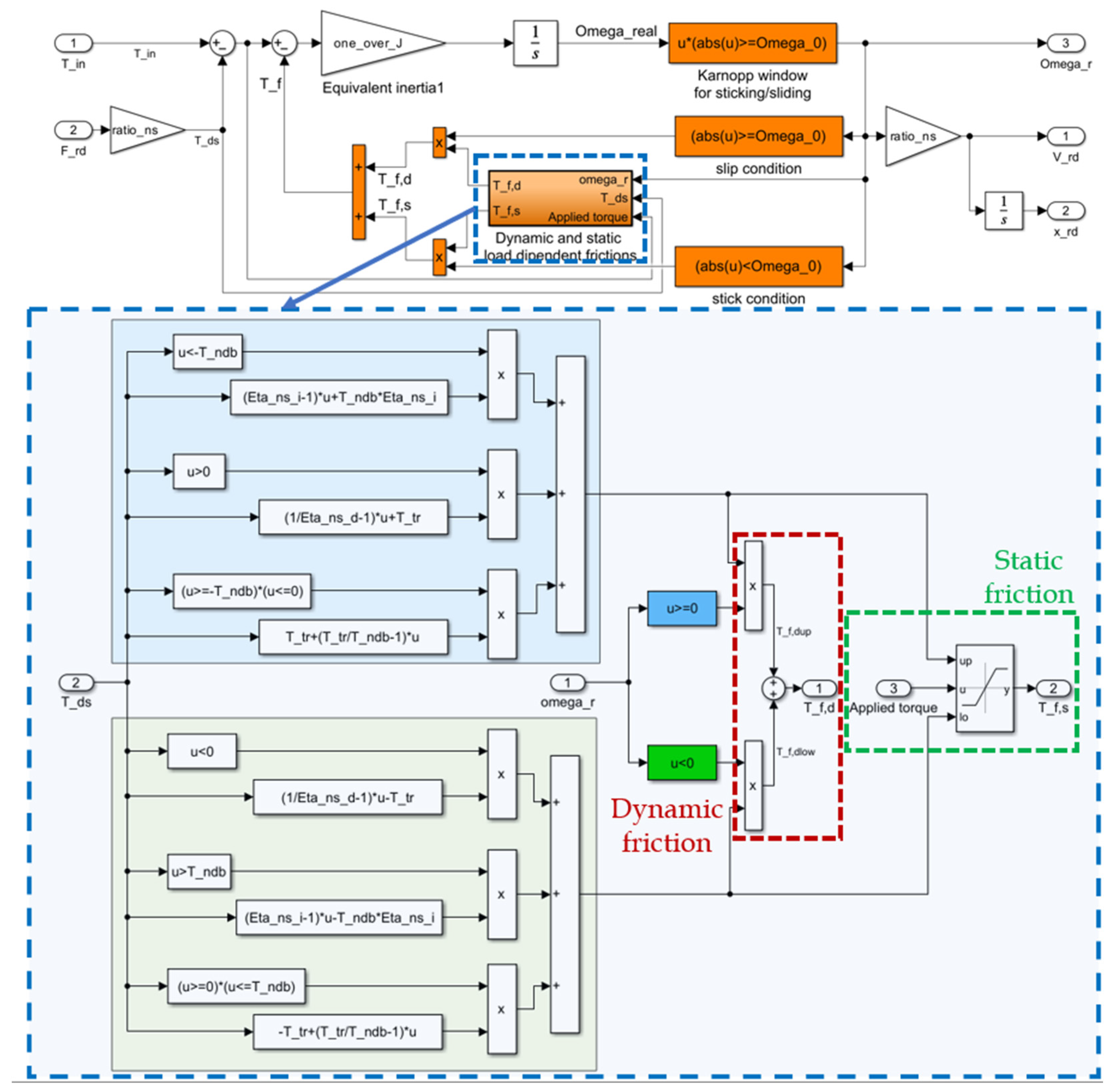
Friction Model Implementation

As previously mentioned, a modified Karnopp friction model [39] has been implemented to represent the true sticking behavior, being the friction curve described with the adoption of engineering parameters, which can be found in manufacturers’ data sheets. This need came from the fact that it is not realistic to only represent friction as a function of the velocity for mechanical transmission [40]. Therefore, the friction torque has been decomposed into two effects:

• A load-dependent effect, which is calculated as a function of either the direct or indirect efficiencies, i.e., in the case of opposing or aiding loads, with respect to the body movement;
• A load-independent effect, which depends on the system’s geometry and lubrication properties.

Thus, this model uses four commonly available parameters, available in most manufacturers’ catalogs, which are the direct efficiency ${\eta }_{NSd}$, the indirect efficiency ${\eta }_{NSi}$, the no-drive back-driving torque $T_{NDB}$, and the no-load driving torque $T_{NLD}$. The transition between sticking and sliding is performed with the aid of a Karnopp window on the sliding speed: when the latter enters inside the window $\left|\omega \right|<{\omega }_0$, the actuator is considered still, and the static friction torque $T_{f,s}$ applies. When the system is in static conditions, $T_{f,s}$ represents the limit static torque, but the actual friction torque applied on the system equals the active net torque in order to obtain a null acceleration and maintain steady conditions. When the net torque increases and reaches $T_{f,s}$, the static limit is exceeded and the system starts moving, exiting the Karnopp window into a dynamic friction situation. According to [40], the dynamic friction torque $T_{f,d}$ is calculated as a function of the downstream torque $T_{ds}$, i.e., the equivalent torque created in the rotational domain by the linear external force on the ball screw nut, coming from the interaction of the actuator rod with the control surface. The value of this torque determines three regions, representing the aiding mode, opposing mode, and a transition situation between the first two situations [40]. The various calculations for the different operating conditions are summarized in

Table 3. Synthesis of dynamic friction calculations with engineering parameters, according to [40].

Mode	Positive Speed	Friction Torque
Aiding	$T_{ds}\mathrm{s}\mathrm{i}\mathrm{g}\mathrm{n}\left(\omega \right)<-T_{NDB}$	$T_{f,d}=\left({\eta }_{NSi}-1\right)T_{ds}+T_{NDB}{\eta }_{NSi}\mathrm{s}\mathrm{i}\mathrm{g}\mathrm{n}\left(\omega \right)$
Opposing	$\mathrm{s}\mathrm{i}\mathrm{g}\mathrm{n}\left(\omega \right)T_{ds}>0$	$T_{f,d}=\left(1/{\eta }_{NSd}-1\right)T_{ds}+T_{NLD}\mathrm{s}\mathrm{i}\mathrm{g}\mathrm{n}\left(\omega \right)$
Transition	${-T_{NDB}<T}_{ds}\mathrm{s}\mathrm{i}\mathrm{g}\mathrm{n}\left(\omega \right)<0$	$T_{f,d}=T_{NLD}\mathrm{s}\mathrm{i}\mathrm{g}\mathrm{n}\left(\omega \right)+\left({\displaystyle \frac{T_{NLD}}{T_{NDB}}}-1\right)T_{ds}$

, while the initial easiest and most inefficient Simulink block implementation is shown in Figure 9.

The block diagram shown in Figure 9 represents the first version of the model implementation, aimed at readability and simplicity: the static and dynamic contributions are both calculated at each time step and summed up by multiplying them by the stick/slip logic condition. This multiplication reflects the inherent nature of the problem: in fact, static and dynamic conditions cannot coexist at the same time since they are mutually exclusive. Actually, only one of the six rows of blocks in Figure 9 should be evaluated at each time step; therefore, the block diagram has been modified adopting a nested IF-THEN structure, as shown in Figure 10. Looking at the activating conditions, a first screening is performed on the slip condition; if the system is slipping (i.e., the speed falls within the Karnopp window), then the speed of the system discriminates which block to activate; otherwise, it is decided by analyzing the sign of the applied torque, that is, the difference between the input torque from the electric motor and the resistant torque coming from the surface attachment (observable in Figure 9). Inside each conditionally activated subsystem, a second nested IF-THEN structure is present, analyzing and discriminating the operating condition between aiding, opposing, or transitioning according to Table 3. In addition, in the case the system is in sticking condition, the friction torque is saturated to the applied torque such that the system remains in adherence if the limit static torque is not reached, but it moves if this value is overcome. Furthermore, the saturation allows the friction torque to be only reactive and not propulsive, leading to unrealistic and not physical results in which the friction torque drives the system.

These measures led to a 12.5% reduction in computational time compared with the initial model implementation shown in Figure 9.

The concept of avoiding repeated operations has been applied throughout the entire model, such as for the evaluation of the sticking condition of the mechanical transmission when the speed enters the Karnopp window, as shown in Figure 9, where the slip condition is evaluated multiple times. The block diagram has been modified in such a way that the evaluation of the sticking/sliding conditions is performed only once, and the result is used to control every conditionally activated subsystem relevant to the static or dynamic friction, adding determinism and univocity to the various alternative conditions.

4.3. Usage of Discrete-Time Integrator

Since the compiled code will be executed with a fixed-step integrator on RT hardware, it is convenient to use discrete-time integrators instead of continuous ones within the model. This approach can sensibly reduce the computational time while introducing little approximation errors in the solution. Different integrator formulations can be selected, such as forward Euler, backward Euler, and trapezoidal. The results obtained with these three formulations have been compared with those given as output by the same model in which continuous integrators were still present, simulated with a 120 kHz frequency (ten times higher than the specific application value to obtain a comparison considering the continuous solution with an increased precision). The evaluation has been carried out on the most dynamic state variable present in the model, i.e., the motor current. From the analyses of the results, it was decided to adopt discrete-time integrators with the forward Euler formulation due to its low relative error, with respect to the solution obtained with continuous integrators. The two solutions are very similar, with a mean relative error of 0.3% and a coefficient of determination greater than 99.99%.

These measures led to a 65.2% reduction in the computational time compared with the model implementation obtained after the modifications described in Section 4.2.

4.4. Introduction of Only Functional Models of Components and Phenomena

Before creating a model optimized for real-time applications, usually, it is better to design it from an architectural point of view. This means that it is paramount to define which subcomponents and/or physical phenomena will be modeled in a physical way and which, instead, are not mandatory to represent the main quantities of interest for the particular application. The first category are those elements that are necessary to allow the model to represent the basic response of the physical system, such as the electric motor, the mechanical transmission, and surface dynamics for the EMA model presented in this paper. The second category includes all those elements that are optional from a model point of view: these components are compulsory in the physical system but are not strictly required in the mathematical model domain.

The choice of what falls in this latter group can be made based on two main aspects. The first involves the evaluation of the representable dynamics in the model, depending on the maximum integration frequency, as described in Table 2. Usually, the physical phenomena of this kind constitute a second-order level of representation of the system behavior: they help in the enhancement of model realism but generally involve high dynamics and, especially for RT applications, overcome the maximum representable frequency. Omitting these phenomena, of course, degrades the accuracy of the model results but to a generally negligible degree.

The second group includes all those elements that have the characteristics of being present in the real system but not usually involved in the majority of normal operations. Examples of such systems can be, for example, mechanical endstops or emergency brakes.

For these kinds of subcomponents and phenomena of the two previously mentioned groups, the physical modeling can be replaced by only functional representation in order to reproduce their effects on the system behavior without having to waste computational power when they are not used. This approach has been applied to the block diagram of the EMA model presented in this paper and will be described in Section 5.

5. Enhancement of the Reference Model

This section describes the enhancements of the EMA mathematical model which have been added with respect to the reference model in Figure 5. This section constitutes the second step of the iterative two-step procedure that has been applied and that led to the final version of the model. The introduction of the various sub-models, which will be described hereinafter, has been alternated with the application of the computational time reduction techniques presented in Section 4, with a recurring sequence of complexity increase and computational burden reduction.

5.1. Loading System Dynamics

As shown in Figure 3, the actuators of the real half-wing of the iron bird are subjected to artificial equivalent aerodynamic loads depending on the phase and maneuver of the simulated flight. These loads are applied by hydraulic actuators properly mounted in such a way as to create a disturbance on the position control loop of the flight control actuators. In order to allow a realistic representation of the load generation, the dynamic description of the loading actuator should be included in the RT model. In fact, this allows the load to be applied to the simulated half-wing actuators with the same dynamics of the physical load generation system on the real half-wing, with the goal of balance and symmetry between the half-wings without incurring instabilities on the flight dynamics simulator.

Since the accurate description of the hydraulic loading system is not paramount for the RT application as it has only a functional meaning, it has been included in the model exploiting the technique described in Section 4.3: it has been represented with a black-box model, i.e., a transfer function of the second order aimed at reproducing the main dynamics of the loading system while concurrently maintaining the minimum computational effort. In order to optimize, as much as possible, the latter parameter, techniques 4.2 and 4.3 have been adopted and implemented by means of a discrete transfer function realized with Simulink built-in blocks.

5.2. Mechanical Endstops

The mechanical endstops have been inserted at both the surface and actuator level, modeled in the same way. Only the actuator endstop implementation will be presented, as depicted in Figure 11. These elements are important if extreme operative conditions are reached, but they generally do not get involved in usual flight simulations. For this reason, they have been considered functional elements as specified in Section 4.3: this means that the endstops have not been modeled with continuous elastic-damping elements but with signal saturations, as shown in Figure 11. In fact, due to their extremely high contact stiffness, elastic endstops generally involve very high frequencies in the endstop force signals, which exceed the maximum reproducible frequency given the RT constraints on the integration frequency.

Figure 11 depicts the block diagram optimized following the points in Section 4.2: the calculations necessary for endstop intervention have been enclosed in a conditionally activated subsystem, whose content is shown in Figure 12. This way, it is evaluated only if the rod’s linear position reaches one of the two endstops; otherwise, the input acceleration signal is transparently transmitted to the integrator. When the actuator reaches the position limit, the actuator acceleration is set to zero according to the logic in

Table 4. Endstop acceleration limitation logic.

Endstop Reached	Input Acceleration	Transmitted Acceleration
Positive	Positive	0
Positive	Negative	Input acceleration
Negative	Positive	Input acceleration
Negative	Negative	0

; the integrator is hard reset to ensure a null output speed. This creates a discontinuity in acceleration, neglecting the impact dynamics. However, this does not create problems in the integration.

Furthermore, the neglected dynamics is really fast considering the endstop stiffness and the integration frequency might not be sufficiently high to describe it, with the consequent risk of creating instability in the solution. Finally, in normal operating conditions, the systems should never reach the endstops; as such, the probability of intervention of endstop models is so low that this assumption is justified.

5.3. Electromechanical Brakes

As for the mechanical endstops, the electromechanical brake action has been added in a functional manner, according to Section 4.3. Its implementation can be observed in Figure 11 and Figure 12: the brake command input is a Boolean variable, which bypasses the evaluation of the endstop contacts and directly resets the acceleration integrator.

5.4. Controller and Sensor Signal Sampling

The developed RT model does not consider the dynamics of the sensors used to close the control loops since their high natural frequencies are not compatible with the RT constraint. However, due to this characteristic, they introduce negligible amplitude modification and phase shift for the expected operating frequencies and do not alter the model response of interest. Therefore, they can be assumed to be zero-order systems. However, digital converter sampling and quantization have been taken into account depending on the characteristics of the electronics. It is worth mentioning that the sampling period of the motor winding current signals has been assumed equal to the integration time step, while that of speed and position signals have been taken as an integer divider of the integration time step in accordance with the effective sampling frequencies of the corresponding loops.

5.5. Two-Dimensional Electric Motor in dq Axes

To implement a representative description of the electric motor dynamics without adding excessive computational burden, it was decided to adopt a two-dimensional approach based on the reduced d-q axes motor model. This approach is coherent with the physics of the permanent magnet synchronous machine (PMSM) employed in the actuator under analysis, in which the common node current is expected to be negligible. Only resistive losses are accounted for as they are expected to be the most prominent parasitic effect in the motor operating range. Figure 13 shows the MATLAB/Simulink implementation of the d-q axes reduced model.

5.6. PHM-Oriented Model Refinements

As anticipated in Section 3.1, the models were prepared to be employed on board an iron bird designed to support the development of prognostics and health management techniques. As such, there was a need to give the model the capability to represent the effects of the most prominent failure modes, along with their possible propagation in time as a function of the actuator usage. Such failure modes were selected according to a PHM-dedicated FMECA (failure mode and effect criticality analysis), performed following the procedures prescribed in [41] and supported by inputs from the industrial partners of the research program, resulting in the choice of representing:

• The occurrence of a turn-to-turn short within one of the PMSM phases (EMTTS);
• The possible onset of static eccentricity within the electric motor (EMSE);
• The distributed degradation of the permanent magnets within the PMSM (EMDMD);
• The incurrence of backlash within the mechanical transmission due to wear (MTBCKL);
• the presence of backlash within the rod end at the interface between the actuator and the control surface due to wear (REBCKL);
• Loss of mechanical efficiency due to jamming onset within the actuator bearings (MTEL).

Most of these failure modes have been described and applied by authors in the past to high-fidelity models [10,42]. Such models are, however, too complex to be suitable for the contemporary execution of multiple simulation instances as is required on the iron bird. As such, it was needed to devise a way to include the description of these degradations without adding unnecessary complexity within the real-time models. To pursue this objective, the failure modes have been divided into three categories. The first is made of the failure modes that can be characterized through simple, zero-order physics-based equations. The second pertains to the failure modes for which some off-model processing and mapping were required. The third, finally, pertains to the failure modes for which it was possible to reduce the complexity through implementation expedients.

Within the first category, it is possible to find the degradation of the permanent magnets within the PMSM and the loss of mechanical efficiency due to jamming onset within the actuator bearings. Both have been described with factors ranging between 0 and 1, proportionally affecting the reduction in the magnetic flux for the former degradation and the variation of the mechanical efficiency of the transmission for the second degradation.

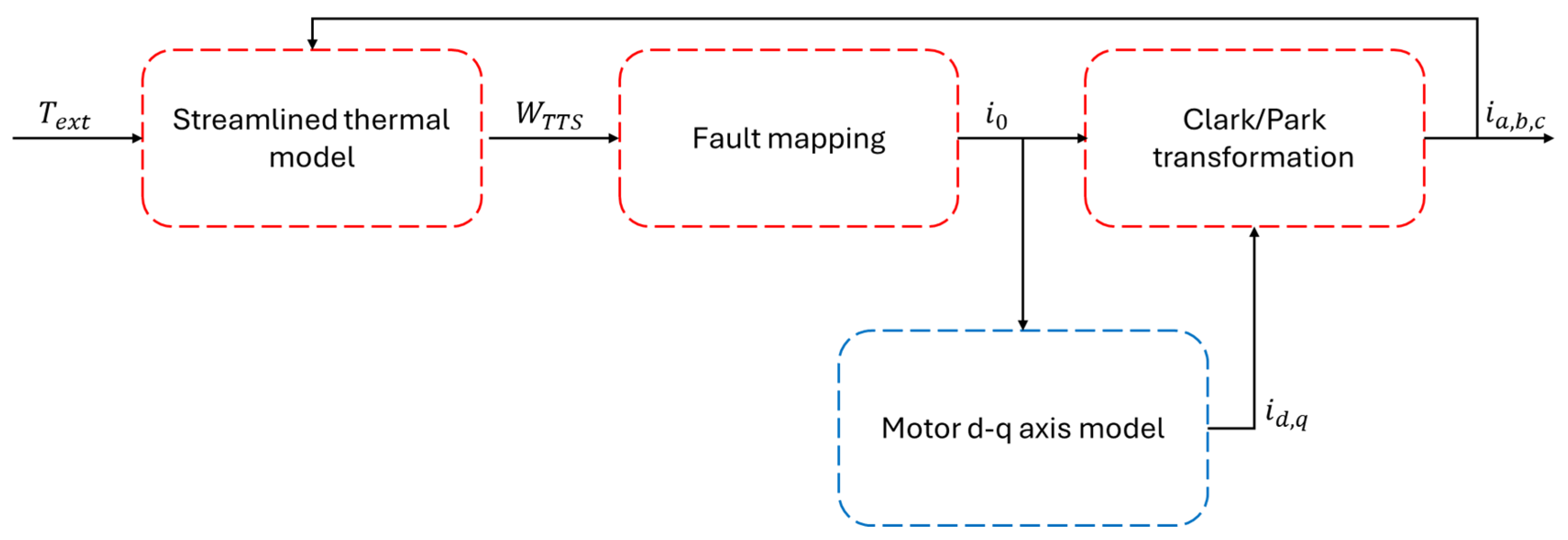
The occurrence of a turn-to-turn short within one of the PMSM phases and the possible onset of static eccentricity within the motor fall within the second category, thus requiring added complexity and off-model pre-processing. The turn-to-turn short is typically described as a reduction in the electrical resistance and inductance of the phase affected by its occurrence. This typically requires describing the dynamics of the three phases, thus introducing additional calculations and dynamics within the model. The key idea to avoid this was found in describing this failure mode by resorting to a map of the faults’ effect on the common node current. As the common node current was not described in the model, its effect has been added to the d-q axis model. As the signals needed to monitor the fault in practice are the phase current signals, the process described in Figure 14 has been applied where the phase currents $\left(i_a,i_b,i_c\right)$ are computed through the Clarke/Park transformation [43] considering the additional common node current $i_0$. A streamlined thermal model, based on the thermal power balance between the copper losses in the motor and the external temperature $T_{ext}$ has been used to estimate the fault size $W_{TTS}$ according to a dependency derived from the Arrhenius law [44]. This approach introduces only the dynamics pertaining to the thermal model, allowing for computing the phase currents through simple zero-order relationships.

A similar approach has been devised for static eccentricity where mappings pertaining to the effects of the fault occurrence on the $\left(i_d,i_q\right)$ pair have been introduced as a function of the fault size and of the rotor angular position.

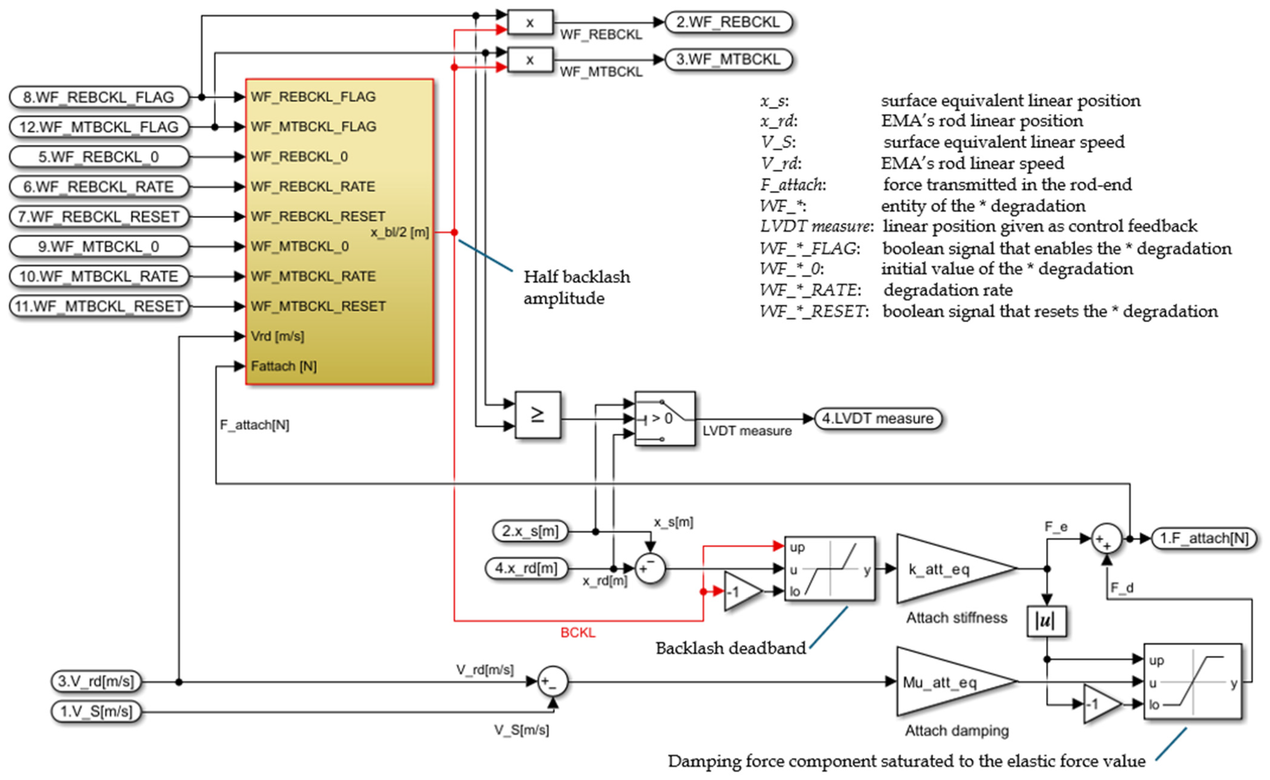
The last two remaining failure modes, the backlash within the mechanical transmission and within the rod end, have been introduced with reduced complexity by paying attention to their implementation, without additional mappings.

Both types of backlashes can be reasonably modeled in a similar way, thus considering a constant (or variable) wear rate multiplying the product between the actuator speed and the external load transferred from the control surface. In principle, the backlash should be applied as a dynamic deadband on the force transfer between the nut and the screw (backlash within the mechanical transmission) and between the actuator and the control surface (backlash in the rod end). This would require providing separate dynamic models of the ball screw components and would significantly increase the number of signals managed by the simulation. At the same time, it is important to notice that while the backlash within the ball screw components can be directly observed by the onboard sensors, the backlash in the rod end cannot since the attachment is positioned downstream of the LVDT sensor employed to close the position control loop.

To allow for both backlash types to be modeled without introducing unnecessary computational load within the simulation, it was decided to follow the implementation proposed in Figure 15. Both wear processes have been described and combined, providing the equivalent backlash signal “BCKL”. Then, as only one failure mode is active at any time, the system is forced to treat this signal as a ball screw-related fault or a rod end-related degradation. In case a rod end backlash is considered, the LVDT model will see the linear position of the actuator (upstream of the equivalent backlash) as its input. Otherwise, if the ball screw backlash is selected, the LVDT model will consider the linear position of the control surface (downstream of the equivalent backlash) as its input, mimicking the effects of either failure mode without the introduction of additional dynamics.

6. Results and Discussion

In this section, the TET and model validation results are analyzed and discussed.

6.1. TET Results

The techniques, simplifications and improvements described in the previous paragraphs have been applied to the initial reference model following the aforementioned two-step approach. The fidelity increase and the computational burden reduction have been alternately applied to the model. The result of such an approach is a series of different models, each one with different characteristics, described phenomena, and specific block implementations.

Table 5. Model improvements and TET progression.

Model	Characteristics	Average TET (µs)	N. of State Variables
1	Reference model as in Figure 5	1.625	8
2	Improved surface variable lever arm model	1.293	7
3	Improved Karnopp friction model	1.435	7
4	Load-dependent friction model Only built-in Simulink blocks used	1.485	7
5	Improved block implementation of the friction model Optimized model settings and compiling options Optimized compiled code	1.180	7
6	More detailed friction model sticking criteria	1.235	7
7	Friction model IF structure implemented (as shown in Figure 10) Continuous integrators replaced with discrete integrators Dynamics of IB loading actuators considered	0.818	9
8	Endstops at surface and actuator levels implemented Backlash between rod and surface attachment implemented Surface pivot simplified friction considered Brake’s conditional logic implemented	0.763	10
9	Position and speed controller loops’ sampling frequencies considered Different sampling rates in EACU for position and speed loops Antialiasing discrete filter added on speed feedback signal Discrete smoothing filter for the speed control loop command added	0.803	11
10	Ideal three-phase inverter description added State variable for rotor angular position for EACU added Improved electric motor dynamics as dq axes Three-phase currents and voltages described through Clarke/Park transforms dq axes motor control considered	1.205	15
11	Iron bird’s loading actuator dynamics transfer function replaced with discrete integrator implementation Interpreted MATLAB functions replaced with built-in blocks Number of Clarke/Park transform minimized Redundant integrators suppressed	0.853	12
12	Optimization of Clarke/Park transforms coding More realistic description of three-phase PDU with abc phases added Degradation models implemented	1.755	20
13	Optimization of degradation models Output abc motor phases filter added	1.745	23
14	Optimization of model implementation and coding Model input and output names and signals coherent with ASTIB requirements	1.675	23
15	Electric motor distributed magnet degradation (EMDMD) fault activated	1.675	23
16	Static eccentricity (EMSE) fault activated	1.675	23
17	Electric motor turn-to-turn short (EMTTS) fault activated	1.825	23
18	Mosfet base drive open circuit (MBDO) fault activated	1.695	23
19	Mechanical transmission backlash (MTBCKL) fault activated	1.705	23
20	Mechanical transmission efficiency loss (MTEL) fault activated	1.705	23
21	Rod end backlash (REBCKL) fault activated	1.695	23
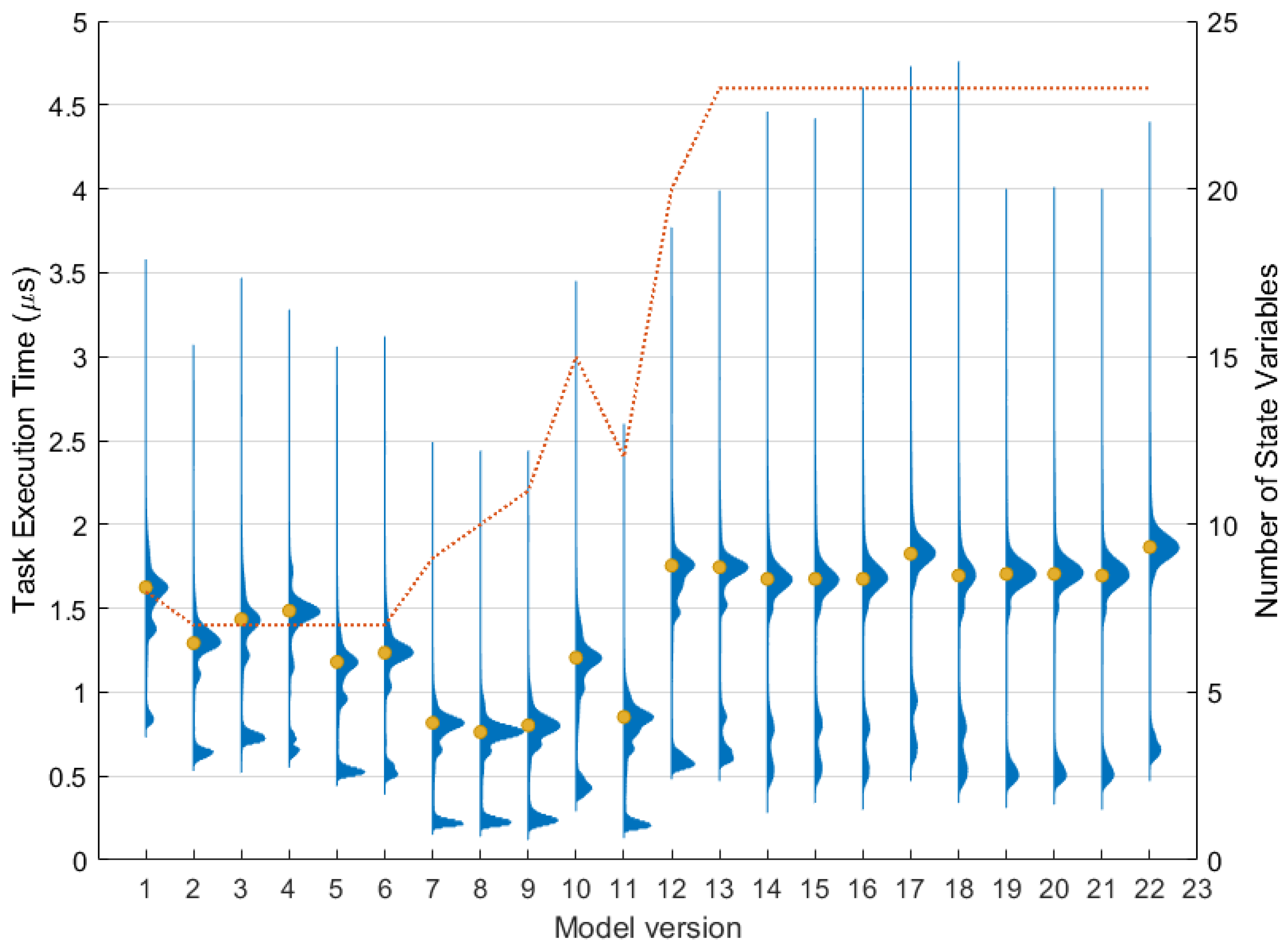
22	All faults simultaneously activated	1.865	23

lists the sequence of model versions showing the average TET and the total number of state variables. Each model version has been executed 100 times, simulating a dynamic command sequence of 3 s aimed to excite and stimulate the various possible configurations contained within the model, with an integration frequency of 12 kHz. The TET value was recorded for the evaluation of each time step. This means that the value of the average TET listed in Table 5 for each model version is the average time required to complete a single integration step. This single value is, however, not fully representative of the effective time taken to evaluate the model as it is necessary to also consider both the jitter phenomenon (as previously mentioned) and the variability in the TET given by the hardware. Figure 16 shows the distribution of the TET for each model version considering the whole set of 100 simulations where the yellow dots represent the average value listed in Table 5: it can be observed that while the majority of the TET distribution lies around the average value, there is also at least another minor peak at smaller TET values. This can be due to those integration time steps involving simple calculi or fewer operations. It is worth highlighting that, in the reference model (V1), the relevance of the lower peak is very low: in fact, in this model, the block diagram was not yet optimized, and numerous avoidable calculations were performed even when not necessary. The optimization of conditionally executed subsystems led to saving substantial computational time, for example, between V4 and V5, and between V6 and V7 when the IF structure was adopted in the friction model. In fact, depending on the instantaneous simulation conditions, some sections of the model could become inactive with the consequent computational effort saving.

The pattern of the two-step process can be observed in Figure 16 where the complexity reduction steps are those involving a reduction in the TET, as between V1–V2, V4–V5, V6–V7, V10–V11, V12–V14, alternated with some model evolution steps in which more phenomena or more detailed descriptions were introduced, as between V2–V4, V5–V6, V9–V10, V11–V12.

An important TET increase was caused by the introduction of a more realistic description of the electric motor (V9 to V10) and the Clarke/Park transformations (V11–V12). The electric motor subsystem contains minimal conditionally activated blocks and runs at the highest integration frequency in the model. Moving from a mono-phase to a 3-phase description introduced more state variables, calculations, and complexity to the model, reflected by the increased TET.

Version 12 of the model was the first to incorporate the degradation modeling previously described in Section 5.6. Models V15 to V21 are simply the last most updated version of the model (V14), with one of the considered degradations activated. Version 22 contains all degradations activated simultaneously. It is interesting to note that all degradations introduce a negligible increase in computational burden, except for the electric motor turn-to-turn fault (V17), which is the main contributor to the TET increase in V22. In fact, the electric motor turn-to-turn short (EMTTS) fault is the most computationally demanding degradation as, when activated, it involves two additional integrators and Clarke/Park transformations. On the other hand, other degradations’ implementations exclude some parts of the block diagram or, alternatively, introduce very simple operations, which do not introduce substantial computational overhead.

Looking at the number of state variables present in the various versions of the model, it can be seen that the proposed two-step approach was successfully applied as it allowed us to increase the model complexity and the number of described phenomena while keeping the TET constrained. In fact, model version 14 represents a quite detailed and complex description of the examined actuator, containing much more phenomena and details than the initial model V1. Nevertheless, this approach allowed us to maintain a TET of the most detailed version comparable with that of the reference model, both with a TET lower than 2 µs, with an average increase of only 3% when no degradations are active, and less than 15% if all degradations are considered concurrently. Moreover, if the model without degradations is needed, V11 can be used, with an average TET reduction of 53%. The model version V11 has been specifically optimized in the TET to ensure the minimal computational cost possible when simulating a full flight on the iron bird. In fact, when the entire half-wing of the aircraft is simulated, 14 actuators need to be RT-simulated in parallel plus the simplified models of the other primary and secondary flight control actuators, mandatory to enable a complete simulation, such as those actuating the ailerons, rudder, elevators, landing gears, and so forth. In this case, it is paramount to minimize as much as possible of the computational overhead to increase the integration failure probability due to overrun conditions.

Figure 17 depicts a portion of the TET measurements in one of the simulations performed with model V14 and graphically represents the meaning of the second histogram peak at lower TET values.

6.2. Model Validation

This section presents the outcome of the obtained real-time model validation against reference data coming from the research program’s partners. The tuning of the RT model parameters was carried out by exploiting the data obtained from the non-real-time high-fidelity Simcenter-AMEsim model, involving 75 state variables and more than 200 parameters, also considering the noise of the sensors. The latter was inserted using a pseudo-random binary sequence, having a magnitude that corresponds to ±2 least significant bits of the analog-to-digital conversion, applied on the voltage obtained from the position LVDT windings, resolver, and phase current sensors [45]. Such a detailed lumped parameter model [46] was used during the model-based design of the real equipment, and it was also exploited to tune the actual control parameters of the real electromechanical actuator. The effect of the noise on the actuator’s sensors on the most significant signals has been neglected in the results presented in this section to better highlight the differences in the response of the two models.

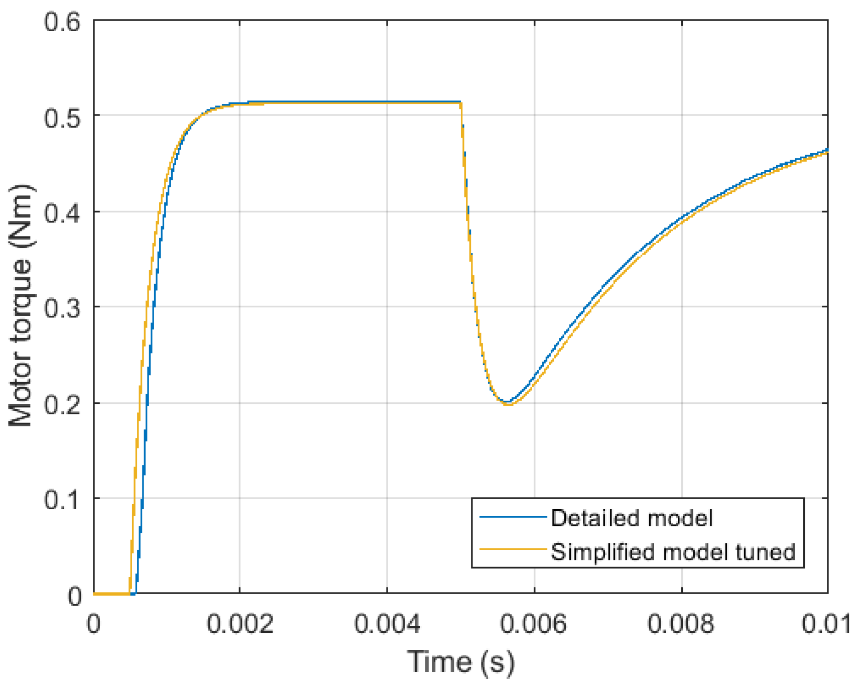
The first step of the tuning process was performed considering the current loop only. A current step demand of 1 A was sent to the controller at 0.5 ms, blocking the rotor shaft to avoid the back-EMF disturbance. The latter was subsequently introduced at 5 ms applying a rotor speed step of 1000 rpm. As observed in Figure 18, the RT model successfully replicates the torque generated by the electric motor, which is directly correlated to the current.

Subsequently, the model was subjected to the speed loop testing phase, which involved a rotor speed step demand of 2000 rpm from 20 ms to 170 ms. To test the disturbance rejection of the regulator, a disturbance torque step of 2.5 Nm was applied on the motor shaft from 100 ms to 150 ms. The results of this second phase of parameter tuning are represented in Figure 19, from which it is possible to observe the good correspondence between the high-fidelity reference model response and the speed obtained from the proposed model. The results consider both the already tuned current loop and the speed loop.

Finally, the complete three-level nested structure of the actuator controller was tested during the last phase, involving the tuning of the rod position loop parameters. To this aim, a position step command of 0.5 mm was sent as input starting at 0.1 s, while a disturbance torque of 160 Nm was applied at 0.3 s on the aerodynamic surface. Also, in this case, the RT model succeeded in replicating the rod position of the more advanced model, as depicted in Figure 20a. Figure 20b illustrates the controller’s internal signals, i.e., the speed command coming from the position loop output and the actual rotor speed. Eventually, Figure 20c shows the effect of the disturbance torque on the aerodynamic surface: the external torque translates to an equivalent linear force on the rod end connection by means of the variable lever arm. The external force introduces minimal displacement variation on the actuator rod, demonstrating its ability to reject disturbances. The oscillations introduced by the torque step can, however, be slightly observed in the speed signal of Figure 20b.

To test the RT model consistency in tracking the high-fidelity response, a simulation was carried out with a more realistic position demand in the presence of a varying aerodynamic torque, shown in Figure 21a. Also in this case the model demonstrates its ability to maintain accuracy under varying operational conditions, further validating its reliability in reproducing the reference behavior. The correspondence between the two signals can be observed not only in terms of surface angle (Figure 21a) and rod position (Figure 21b), but also considering internal fast dynamics such as that of the motor current (Figure 21c).

It is worth noting that such an accurate representation of the main dynamics in presence was obtained with a much lighter model. To get an approximated estimate of the computational time saving realized with the RT model, the scenario shown in Figure 21 was repeatedly simulated with both the RT and the high-fidelity models on the authors’ personal computer, as the reference model was too computationally heavy to be run on the RT hardware. Through this analysis, the RT model achieved comparable results with that of the high-fidelity model, while reducing by approximately 93% the computational effort.

The tuned model was finally compared with an experimental response of the actual actuator provided by the research program partners. Depicted in Figure 22, the provided data included only the surface deflection when a full stroke step command is demanded to the controller in both directions. The RT model shows a good correlation with the experimental data, validating its accuracy and reliability in replicating the actuator’s dynamic response and allowing for its implementation on the iron bird framework.

6.3. Limitations and Uncovered Aspects

Despite the strengths of the proposed real-time modeling approach, several aspects remain unaddressed and will require further refinement for future development of the current research.

One limitation concerns the validation of the mechanical impedance of the position-controlled actuator, i.e., its dynamic stiffness, which is characterized by the frequency response of displacement to the applied force. Additionally, the current implementation does not extend to the simulation of higher-frequency dynamics, such as detailed kinematics with separated motion of each link, pulse-width modulation (PWM), and sensor signal conditioning, although these aspects could be incorporated if permitted by hardware constraints [45].

Another simplification concerns the modeling of the DC link, which is currently assumed to behave as a perfect voltage source. Similarly, thermal effects are not fully accounted for as the present model estimates heat generation from energy losses but does not simulate temperature distribution across the different EMA subcomponents and its impact on system behavior. While implementing an n-body thermal model would be technically feasible, given the relatively small time constants and the well-defined coupling effects on motor winding resistance, power transistor switching losses, mechanical transmission friction, and magnet induction, obtaining accurate parameters remains a significant challenge and represents the main reason why this aspect has been not considered in detail in this paper.

Furthermore, the model does not explicitly account for power electronics behavior at a detailed level, such as switching and conduction losses under temperature variations, nor does it consider the time delays associated with transistor switching in the inverter circuitry.

All these points represent potential areas for future development to enhance system-level reliability analysis and simulation fidelity.

7. Conclusions

The decarbonization of air transport presents a significant challenge that requires the integration of innovative and mature solutions. The transition toward more electric aircraft is a key enabler for achieving greener, safer, and more cost-effective aviation. In this context, the ASTIB CleanSky2 program aims to develop innovative aircraft demonstrator platforms for regional aviation (hybrid iron bird), focusing on the integration of advanced electromechanical actuation systems, digital flight controls, and more efficient aerodynamics to enhance aircraft performance, reduce environmental impact, and facilitate certification through advanced real-time simulation and hybrid testing approaches.

This study focused on the development of wingtip and winglet electromechanical actuators real-time models to be run on the iron bird to enable a realistic and complete flight simulation. The hybrid iron bird approach, combining real and virtual components, has proven to be an effective intermediate step toward full virtual testing environments. By leveraging two-step real-time modeling techniques, including computational cost reduction strategies and incremental model refinement, the developed EMA models successfully balance accuracy and computational efficiency. The presented work demonstrated the feasibility of high-fidelity RT simulation, obtaining a good response accuracy with respect to both off-line high-fidelity models and experimental data, with a substantial saving of the computational cost.

The advancements presented in this work contribute to the broader adoption of virtual testing methodologies, facilitating regulatory acceptance and accelerating the transition to next-generation aircraft with enhanced performance and sustainability.