Article

Deep Neural Network for Valve Fault Diagnosis Integrating Multivariate Time-Series Sensor Data

The Department of Mechanical, Robotics and Energy Engineering, Dongguk University, Seoul 04620, Republic of Korea
*
Author to whom correspondence should be addressed.
Actuators 2025, 14(2), 70; https://doi.org/10.3390/act14020070
Submission received: 18 December 2024 / Revised: 31 January 2025 / Accepted: 3 February 2025 / Published: 5 February 2025
(This article belongs to the Section Actuators for Manufacturing Systems)

Abstract

:
Faults in valves that regulate fluid flow and pressure in industrial systems can significantly degrade system performance. In systems where multiple valves are used simultaneously, a single valve fault can reduce overall efficiency. Existing fault diagnosis methods struggle with the complexity of multivariate time-series data and unseen fault scenarios. To overcome these challenges, this study proposes a method based on a one-dimensional convolutional neural network (1D CNN) for diagnosing the location and severity of valve faults in a multi-valve system. An experimental setup was constructed with 17 sensors, including 8 pressure sensors at the inlets and outlets of 4 valves, 4 flow sensors, and 5 pressure sensors along the main pipe. Sensor data were collected to observe the sensor values corresponding to valve behavior, and foreign objects of varying sizes were inserted into the valves to simulate faults of different severities. These data were used to train and evaluate the proposed model. The proposed method achieved robust prediction accuracy (MAE: 0.0306, RMSE: 0.0629) compared to existing networks, performing on both trained and unseen fault severities. It identified the location of the faulty valve and quantified fault severity, demonstrating generalization capabilities.

1. Introduction

Valves regulate the flow and pressure of fluids in mechanical systems and are components utilized across various fields. Malfunctions in these components can significantly degrade system performance, reducing productivity and wasting resources. In large, complex systems where numerous valves are integrated into various devices and interact with each other, even a single valve malfunction can degrade the overall system’s performance [1,2,3]. In such scenarios, rapid and accurate fault diagnosis is crucial. However, the complex system structure and diverse operational environments make manual valve fault diagnosis highly challenging [4,5,6,7,8,9].
Automated fault diagnosis for components such as valves in mechanical systems is vital for maintaining system performance and predicting its remaining lifespan. This field has seen significant advancements, particularly through the application of artificial intelligence (AI) [10,11,12], with two main methodologies: model-based and data-driven approaches [13,14,15,16,17].
Model-based methods utilize mathematical models of input and output signals, enabling fault diagnosis with small datasets [13,18]. For example, T Wang et al. proposed an adaptive robust fault-tolerant controller based on a dual-valve fault model system to address faults and nonlinearities in dual-valve hydraulic systems. This controller enables effective and precise motion control through real-time fault detection and controller reconfiguration [19]. X Jiang et al. utilized a fault diagnosis and analysis model based on extended Kalman filter banks to diagnose solenoid valve faults in electronically controlled air suspension systems [20]. H. Tian proposed a physical model-based approach to quantify the severity of stiction severity, a common fault in solenoid valves, using temporal features of solenoid coil driving current [21].
However, model-based methods have inherent limitations, such as requiring prior knowledge of the system’s physical model [22]. These methods often fail to fully capture parameter changes like diameter reduction or friction coefficient variation caused by pipe aging under real-world conditions. This discrepancy becomes more pronounced when experimental conditions differ from actual operating environments, leading to reduced diagnostic accuracy [23,24].
In contrast, data-driven methods leverage diverse experimental datasets to learn unique patterns, enabling more accurate fault diagnosis. These methods are particularly effective in addressing issues arising from complex system structures and long-term environmental changes [25]. As a result, they have been widely adopted for diagnosing faults in complex mechanical systems involving valves. For instance, D. Ma et al. utilized a support vector machine (SVM) to diagnose solenoid valve faults [26], while H. Cui et al. analyzed patterns to diagnose reciprocating valve faults using SVM [27]. Additionally, Xiao et al. applied convolutional neural networks to detect abnormal fault signals in reciprocating compressor valves [28]. FY Guo et al. proposed a transfer learning-based convolutional neural network (TCNN) approach for fault diagnosis of reciprocating compressor valves [29].
However, data-driven approaches face inherent limitations. Their performance heavily depends on the availability of large and high-quantity datasets, which may be difficult or costly to obtain in real-world applications. Moreover, these methods often struggle to generalize to unseen fault scenarios, particularly when the pre-learned datasets do not cover the full range of potential fault conditions. Consequently, there is a pressing need to propose systems capable of flexible and accurate diagnostics for various fault scenarios in complex systems with multiple valves. Additionally, developing new fault diagnosis systems that perform well on unseen fault scenarios is essential [30].
This study aims to address the aforementioned challenges in complex structural systems, particularly for valve fault diagnosis, by proposing a data-driven deep learning fault diagnosis network that can simultaneously identify fault location and severity. By predicting system performance degradation, the proposed approach allows for more efficient and cost-effective system management, while considering the remaining lifespan [31,32,33,34]. Notably, it enables flexible diagnostics even for unseen fault severities by adopting a fault severity prediction framework instead of simple classification. By predicting the fault severity for each of the four valves operating simultaneously in an experimental setup, this method quantitatively evaluates fault location and severity. Additionally, it estimates the fault severity for previously unseen severities. This enhances diagnostic reliability and provides a flexible and efficient diagnostic network capable of addressing varying fault severities.
To this end, an experimental apparatus simulating a structural system with multiple valves was developed. Using experimental data, a method is proposed to diagnose faults in multi-valve systems. The specific goals of this study are as follows:
  • This study targets complex multi-valve systems by constructing experimental apparatuses, collecting data, and proposing diagnostic methods for faults in systems with multiple interconnected valves, in contrast to traditional studies on single valves or simpler systems.
  • The proposed method is designed to not only detect the presence of faults but also accurately identify the faulty valve and simultaneously assess fault severities.
  • This study aims to predict fault locations and fault severities, enabling flexible diagnostics for fault locations and unseen fault severities.

2. Experimental Setup and Dataset

To collect the multivariate time-series data to serve as input for the proposed network. We constructed the experimental apparatus shown in Figure 1. The experimental setup consists of a water pump, 13 water pressure sensors, 4 flow sensors, 4 nozzles, a main valve, and 4 valves, each equipped with its own motor for control. The dataset used in the proposed network is collected through this system. Figure 2 shows the piping and instrumentation diagram (P&ID) of the experimental setup, indicating the locations of the pump, sensors, nozzles, and valves.

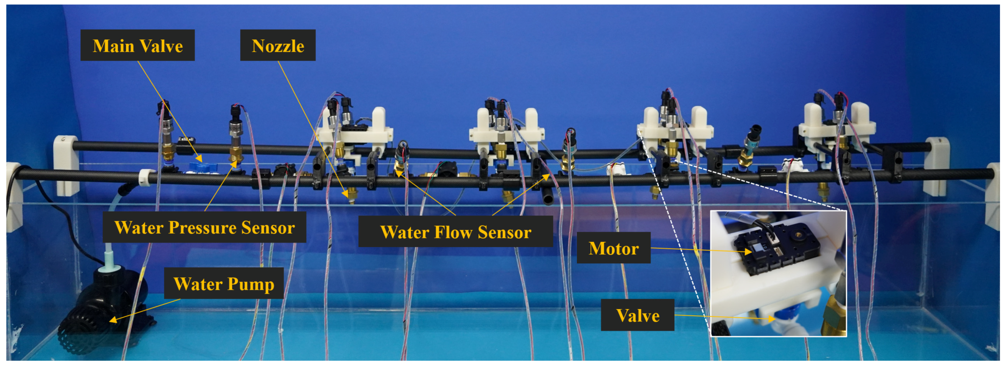
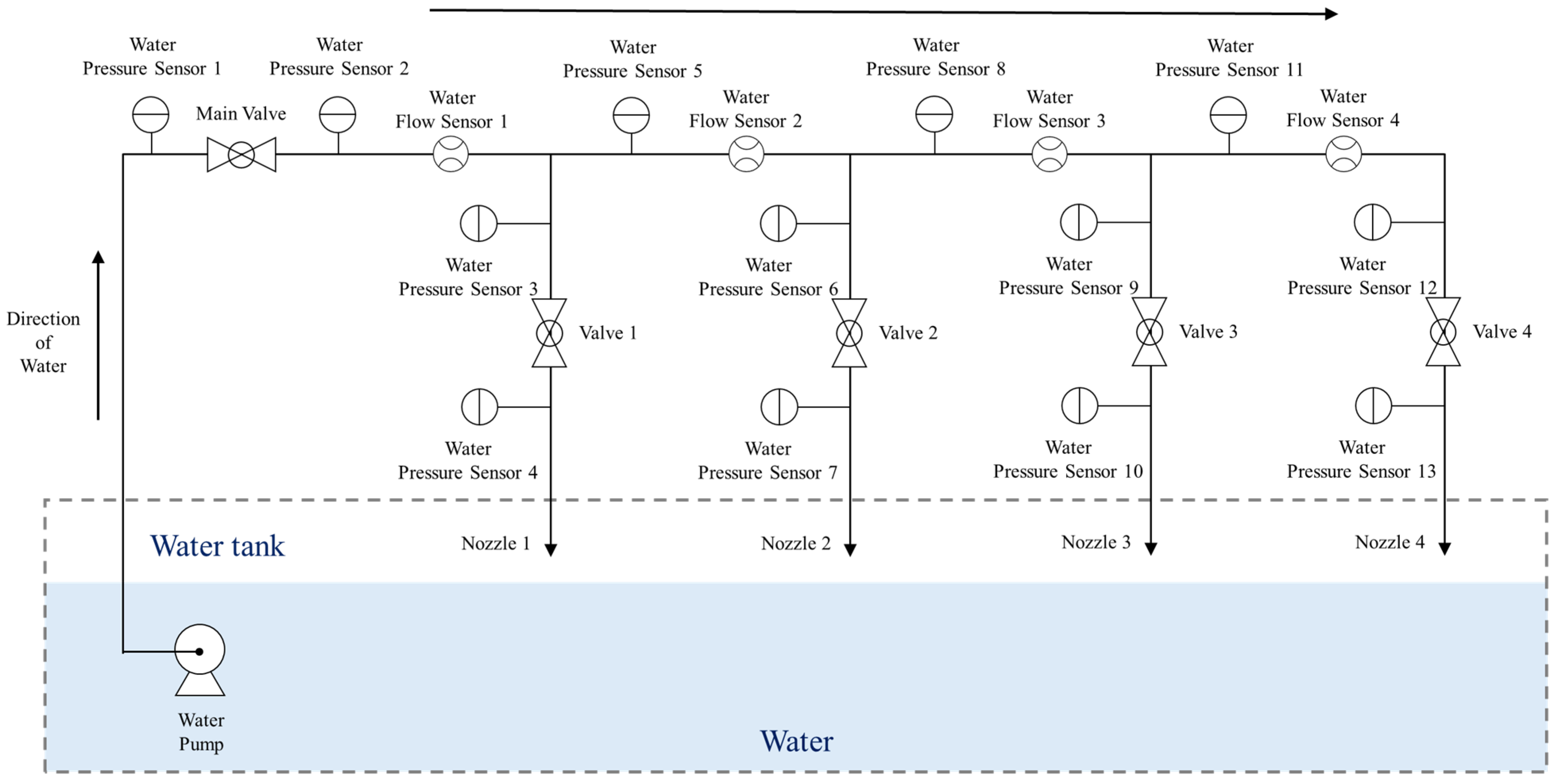
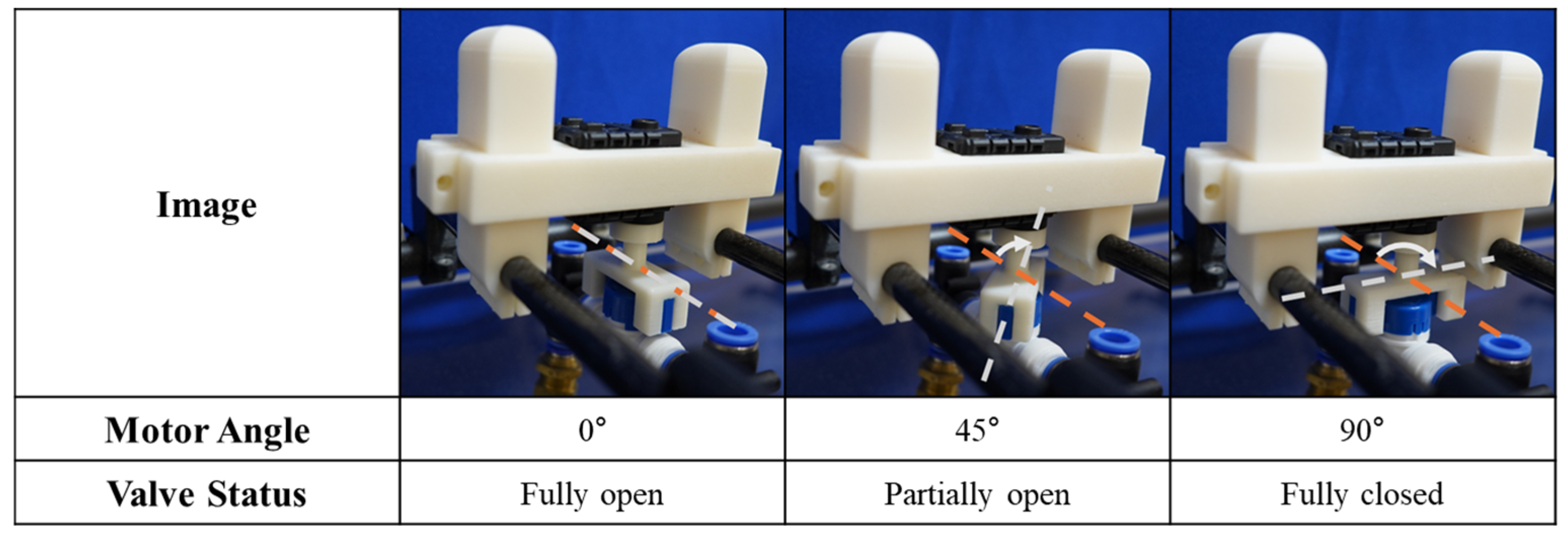
2.1. Experimental Setup

We fabricated an experimental apparatus to emulate a mechanical system regulating water flow. Figure 1 shows the fabricated device, and Figure 2 presents its P&ID. The designed experimental apparatus consists of a water pump (DCP-15000, Jebao, Zhongshan, China) to supply water from a tank to the main pipe, a main valve to regulate water flow in the main pipe, and 4 valves to adjust the water flow when supplied from the main pipe. Each valve is connected to a dedicated nozzle, resulting in a total of 4 nozzles.
Water pressure sensors (SS207 series 30 psi 2 bar gauge) are installed at the inlets and outlets of all 4 valves to measure pressure variations during valve operations. To monitor the water flow and pressure supplied to each nozzle, 4 flow sensors (SEN0217, YM-401A) and 5 pressure sensors are distributed along the main pipe. In total, the system incorporates 13 pressure sensors and 4 flow sensors into the sampling data at 100 Hz.
Water flows through the main pipe and is distributed to the inlets of the 4 valves arranged in parallel, with each valve independently supplying water to its respective nozzle. While this parallel configuration allows for independent valve control, a malfunction in one valve can affect the water pressure and flow in the entire system. For example, if foreign particles obstruct the first valve, less water is supplied to its outlet, resulting in lower outlet pressure and higher inlet pressure. This disruption propagates to the main pipe, leading to increased water pressure and reduced flow. The experimental setup is designed to observe these variations in water pressure and flow caused by valve operations and to collect datasets for training the proposed network.
The operational valves in the system are equipped with motors (Dynamixel AX-18A, Seoul, Republic of Korea) that allow precise control of the opening and closing levels of the ball valves. The ball valves used have an opening range of 0° to 90°, with an inlet and outlet diameter of 10 mm. The motor provides a resolution of approximately 0.3°, enabling precise adjustment of the valve’s opening degree within the 0° to 90° range. When the valve is open (0°), water Tflows through the outlet, and as the valve closes (approaching 90°), the water supply gradually decreases. Figure 3 illustrates the operation of a ball valve controlled by the motor, showing three states: fully open, partially open, and fully closed. By attaching a motor to the top of the ball valve, this setup enables precise monitoring of the valve’s opening degree during experiments and allows for automated operation of the valve.

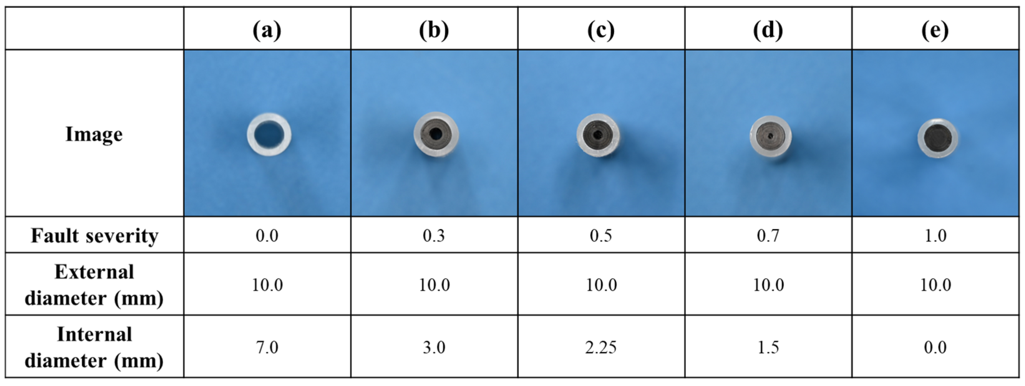
2.2. Determination of Fault Severity in Valves

In general, one of the primary causes of valve fault is scale formation. Scale refers to the deposits that accumulate on the surfaces of pipes or equipment due to factors such as pressure conditions, acidity, or mechanical friction. Scaling can significantly impact both the operation of valves and the flow of fluids [35,36,37]. Changes in water pressure within a pipe directly affect its condition. When scale deposits accumulate inside a pipe, they reduce the pipe’s internal diameter, leading to pressure variations within the pipe [38,39].
Valve faults were simulated by inserting foreign objects into the outlet tube to mimic scale formation. By varying the size of the foreign objects, different fault severities were implemented, enabling the reproduction of various fault levels. For a normal valve, water flows smoothly when the valve is open. However, in a faulty valve where the outlet is blocked by foreign objects, water flow is obstructed even when the valve remains open, resulting in a mismatch between the valve’s operation and the actual water flow. Through this approach, we simulated valve fault conditions.
In this experiment, a significant pressure drop was observed at the valve outlet where a foreign object was inserted, resulting in an internal diameter of 3.0 mm. This was defined as the onset of fault, as pressure reduction in laminar flow due to the decrease in internal diameter was quantitatively analyzed using Equation (1) [40]:
p = 32 μ l D 2 V
where μ is the dynamic viscosity coefficient and l is the length of the tube. D represents the diameter of the tube, and V represents the velocity of the fluid.
Additionally, a secondary fault point was defined at an internal diameter of 1.5 mm, which is the midpoint between the fully blocked tube (0.0 mm) and the initial fault point (3.0 mm). Thus, four fault scenarios were considered in this experiment, with internal diameters of 7.0 mm (normal state), 3.0 mm (initial fault), 1.5 mm (secondary fault), and 0.0 mm (complete fault). These were classified as 1, 2, 3, and 4, respectively. This classification was normalized and rounded to represent fault stages on a scale from 0 to 1.
Figure 4 visually shows the normal valves and the valves corresponding to each fault severity used in the experiment. Additionally, to test the fault diagnosis performance for fault severities not included during the training phase, a validation valve with an internal diameter of 2.25 mm (midway between 1.5 and 3.0 mm) was generated.
Furthermore, to further validate the generalization performance of the proposed network, linear interpolation was applied between (a) and (b), (b) and (c), (c) and (d), and (d) and (e). Fault severities of 0.1, 0.2, 0.4, 0.6, 0.8, and 0.9 were assigned, and the interpolated valves were included in the validation dataset (refer to Table 1).
In this manner, although linear interpolation was applied between each reference valve, the resulting relationship between fault severity and the valve’s internal diameter ultimately shows a nonlinear trend. This is because the pressure drop equation (Equation (1)) is not linear with respect to the valve’s internal diameter. Table 1 provides an explanation of the fault severity and the corresponding valve outlet diameter for each valve.
Figure 5 presents examples of datasets obtained from the experiment, illustrating changes in sensor values corresponding to the operation of valve 1. In the case of a normal valve, sensor values show a tendency to increase or decrease depending on the valve’s operation. However, when a foreign object is inserted into the outlet, causing the valve to become completely faulty, the outlet is entirely blocked regardless of the valve’s operation. Consequently, no significant changes in sensor values are observed. By analyzing the changes in sensor values when foreign substances are present in the valve outlet, it is possible to determine the fault severity and location of the valve.

2.3. Dataset

In the experimental setup developed herein, the changes in water pressure and flow rate were recorded based on the opening and closing of the 4 valves. Data were collected to compare sensor readings from the multi-valve operating system under normal valve conditions with those under fault conditions. When collecting data, the motors attached to the valves were manipulated to operate in increments of approximately 6°. To ensure clarity during training, data samples corresponding to fully open or fully closed valve states were excluded.
The valve operation sequence began from an open state (23°), proceeded to a closed state (64°), and then returned to the open state (23°). Such valve operations are divided into three categories: one valve operation, two valve operations, and three valve operations, out of the four valves. Table 2 presents the valve numbers corresponding to the number of operating valves, and data were collected for each scenario listed in Table 1.
For the non-operational valves, seven states were defined: 23°, 29°, 35°, 41°, 47°, 53°, and 59°. Unlike the operating valves, non-operating valves do not undergo the process of opening and closing. Instead, they remain static at a defined angle throughout the data collection process. Table 3 shows the dataset configuration used in the training and testing processes. Data collection was conducted following the aforementioned methods and Table 3. During this process, it was assumed that only one of the four valves was in a fault state.
To further ensure the distinctiveness of the training and testing datasets, the starting angle of the non-operating valve was intentionally set differently between the two datasets. In the training dataset, the non-operating valve angles were limited to 23°, 35°, 41°, 47°, and 59°, while in the testing dataset, the angles included 29° and 53°. This distinction was implemented to evaluate the network’s ability to generalize to conditions not explicitly seen during training.
Through this procedure, 1,345,000 training data samples and 1,697,400 testing data samples were obtained. These data samples were used as inputs for the network, with each sample consisting of motor rotation values representing the opening and closing states of the 4 valves and readings from 17 sensors. The data were collected at a frequency of 100 Hz, with each sample representing a 1 s sequence of collected data. Thus, each data sample has a shape of (100, 21).

3. Methods

3.1. Training Model Based on 1D CNN

The 1D CNN model exhibits excellent performance in handling one-dimensional data such as audio, text, and time-series data. When compared to other neural networks, the 1D CNN has demonstrated superior performance in classification and regression tasks [41,42,43,44,45,46]. Based on this 1D CNN model, a network was designed to predict valve fault locations and fault severities using sensor data and valve state data. Figure 6 and Table 4 provide a detailed illustration of the proposed network’s structure.

3.1.1. Composition of Input and Output Data

The input data consist of time-series data reflecting the state of the valve system and are defined as follows:
X = x i , t i 1 , 2 , , N + M , t { 1 , 2 , , T } }
where N represents the number of sensor values, which is 17, and M denotes the number of valve state values, which is 4. T   indicates the sample length for each variable, which is 100. x i , t indicates the value of the i -th input (sensor or valve state value) at the t -th time step. Therefore, the input data consist of a total of N + M = 21 variables, all processed as time-series data collected at 100 Hz. Since sensor data were collected at 100 Hz, each variable contains 100 data points for every second. Combining the data points from all variables over a 1 s interval results in a single data sample comprising a total of 2100 data points. These data samples are randomly shuffled and directly used as inputs to the network without any additional preprocessing or filtering, effectively minimizing the time and cost associated with data preprocessing [47,48].
The input data are processed through the proposed network to generate outputs that simultaneously predict the fault location and fault severities of the valves. The output values are defined as follows:
Y ^ = { y ^ 1 , y ^ 2 , y ^ 3 , y ^ 4 }
where y ^ i represents the fault severity of the i -th valve, defined as a value between 0 and 1, thereby simultaneously indicating the fault location and the fault severity of each valve.

3.1.2. Network Composition

The proposed network consists of four 1D convolution (1D Conv) blocks and three fully connected (FC) layers, designed to effectively learn the temporal features of the data for valve fault diagnosis. Each 1D Conv block has 512, 1024, 2048, and 4096 channels, respectively, and extracts key features through each layer, followed by max pooling to reduce the data size [49,50]. The max pooling layer efficiently compressed the data while retaining important features and is defined as follows:
s k l j = m a x   { y k l j 1 · s s + 1 , , y k l [ j · s s ] }
where s s represents the size of the pooling window, and s k l j is the output value of the j -th pooling window.
Before transitioning from the final 1D Conv block to the FC layers, average pooling is applied to summarize the average information of the entire dataset. The average pooling operation is defined as follows:
s k l j = 1 s s m = j 1 · s s + 1 j · s s y k l [ m ]
where s k l j represents the average value of the j -th pooling window. These pooling operations reduce the spatial size of the data while passing key features to subsequent layers without loss [51].
In each layer of the 1D CNN [52], weights w i k l 1 and bias b k l are learned based on the input data to extract features reflecting the state of the valve system. The k -th input value in the l -th layer is calculated as follows:
x k l = b k l + i = 1 C ( l 1 ) c o n v 1 D ( w i k l 1 , s i l 1 , P )
where C ( l 1 ) is the number of channels in the previous layer, P represents the zero-padding value, and c o n v 1 D denotes the 1D convolution operations. The intermediate output value is calculated by applying the activation function f ( · ) as follows:
y k l = f ( x k l )
This network learns the nonlinear relationships in valve system data through this feature extraction process, enabling accurate fault diagnosis and fault severity assessment.

3.1.3. Training Process

The proposed network uses mean squared error (MSE) as the loss function to enhance the accuracy of fault severity predictions. The loss function is defined as follows:
L M S E = 1 n i = 1 n ( y i y ^ i ) 2
where n is the total number of training data samples, y i represents the actual fault severity of the valve, and y ^ i denotes the predicted fault severity of the valve. Through this loss function, the proposed network is trained to improve the accuracy of fault severity predictions for the valves.
The deep learning approaches were trained using an Adam optimizer with a 0.0001 initial learning rate and with the MSE loss used as a loss function. Models were trained with batch sizes of 256 and up to 50 epochs on an RTX 3090 Ti GPU. The training time for this network was approximately 44 min per epoch, resulting in a total training time of approximately 37 h for 50 epochs. Additionally, the network’s average inference time is found to be 0.75 ms.

3.2. Testing with Trained and Unseen Severities of Valve Faults

This section validates the performance of the trained 1D CNN model. The test data include not only the fault severities used during training but also the ‘unseen’ fault severities of 0.1, 0.2, 0.4, 0.5, 0.6, 0.8, and 0.9, as shown in Figure 4 and Table 1 and Table 3. This evaluation determines whether the trained network can successfully predict unseen fault severities in a multi-valve system. The results provide a critical indicator of whether the trained network demonstrates generalized performance in a multi-valve operating system.

4. Experimental Results and Discussion

To quantify the results of the analysis, the evaluation metrics of mean absolute error (MAE) and root mean squared error (RMSE) were utilized as follows:
M A E = 1 n i = 1 n | y i y ^ i |
R M S E = 1 n i = 1 n ( y i y ^ i ) 2
The performance of the proposed method was evaluated by quantifying the difference between the predicted and ground truth fault severities. Additionally, since this involves comparing the difference between the actual and predicted values, the smaller these values, the more accurate the predictions of the valve fault severities.
Table 5 represents the average MAE and RMSE that were calculated by summing up the individual MAE and RMSE values of the four valves and then taking the average. This refers to the difference between the actual fault severity of the valve and the predicted fault severity, where a smaller difference indicates a higher similarity between the predicted value and the ground truth value.
Using the proposed network, the fault severity for each valve is predicted, after which the MAE and RMSE are calculated by comparing the predicted values with the ground truth values for each valve. The four individual results are summed and averaged to present the overall result.
The ‘Whole case’ row includes not only observed fault severities during training but also cases that were not observed or ‘unseen’ during training. The results show an MAE of 0.0306 and an RMSE of 0.0629. The ‘Only severities used during training’ row displays results for testing only the valve fault severities in Figure 4a,b,d,e that were trained as faults. These fault severities, included in the training data, exhibit the highest accuracy with an MAE of 0.0024 and an RMSE of 0.0059.
The ‘Only severities used during testing’ row represents results when testing only ‘unseen’ fault severities that were not used during training. Although achieving lower accuracy than the trained fault severities, it still demonstrates significant results with an MAE of 0.0467 and an RMSE of 0.0954. These outcomes indicate that the proposed method effectively diagnoses valve faults, including those not encountered during the training process. This achievement is attributed to the construction of a valve fault diagnosis model that outputs a continuous fault severity ranging from 0 to 1, instead of identifying specific severities of valve faults. By utilizing fault severities rather than simple fault classification, this approach enables the characterization of the severity of each valve’s malfunction.
Figure 7 illustrates a bar graph showing the mean and standard deviation of the differences between predicted and actual valve fault severities. The bar length represents the average value, with the average difference consistently below 0.040, indicating a high level of accuracy as the values were close to 0. The black error bars in this graph represent the standard deviation around the mean value. Since the results did not follow a Gaussian distribution, the standard deviation was computed based on the mean. The bars above the mean point indicate the standard deviation values beyond the mean, while the bars below the mean point represent the standard deviation values below the mean.
As shown in Figure 7, among the four valves, valve 1 has the least error. This is due to the experimental setup where water is supplied through a single main pipe using one pump. The operation of the valves at the front directly influences the pressure and flow of water supplied to the valves at the back. For instance, when valve 1 is closed, water does not flow through the nozzle, thus causing an overall increase in pressure within the pipe behind valve 1. Consequently, in situations where multiple valves are operating in a complex manner, the opening and closing of the valves leads to intricate changes in pressure and flow. This complexity introduces confusion, introducing challenges in accurately predicting fault severity for valves farther downstream. Furthermore, during the assembly of the experimental apparatus, the main pipe experienced diameter changes due to the connector used to attach the flow sensor. As the flow decreases toward the end of the main pipe, two fault severities of flow sensors were used considering their measurement range. Due to the flow sensor between valve 1 and valve 2, the flow sensor before valve 1 changes. At this time, the sudden change in the pipe’s diameter would have altered the water flow, causing confusion in accurately predicting the fault.
To demonstrate the superior performance of the proposed network (1D Conv blocks + FC layers) over other networks, we set FC layers, recurrent neural network (RNN), renowned for its excellent performance in time-series data analysis, and its more advanced model, long short-term memory (LSTM) [53], as comparison networks. Additionally, we also included the simple regression models, support vector machine (SVM), and random forest (RF), in the comparison group. The results can be seen in Table 6. The comparison results include not only the fault severities of valves used during the training but also those used only in the test process. The proposed network showed the best results with an MAE of 0.0306 and RMSE of 0.0629. The LSTM model showed the next best performance after the proposed network with an MAE of 0.0434 and an RMSE of 0.0909, while the RNN showed a performance of an MAE of 0.0807 and an RMSE of 0.1176. The FC layer showed the lowest result among the deep learning comparison groups with an MAE of 0.1171 and an RMSE of 0.2560. The SVM showed an MAE of 0.2447 and RMSE of 0.3550, and the RF showed results of MAE of 0.2145 and RMSE of 0.3877, indicating lower accuracy than the deep learning networks.
Notably, the proposed model demonstrated superior fault diagnosis performance on data not used during training compared to most of the comparison networks. Despite being tested exclusively on untrained fault severities, the proposed model outperformed most of the comparison networks, which were tested on datasets including trained fault severities. These results indicate that the proposed model is capable of effectively diagnosing fault severities even under ‘unseen’ conditions.
Table 7 presents the results of various configurations of the input sensors for the proposed network. The configurations of the network input used for result comparison are as follows:
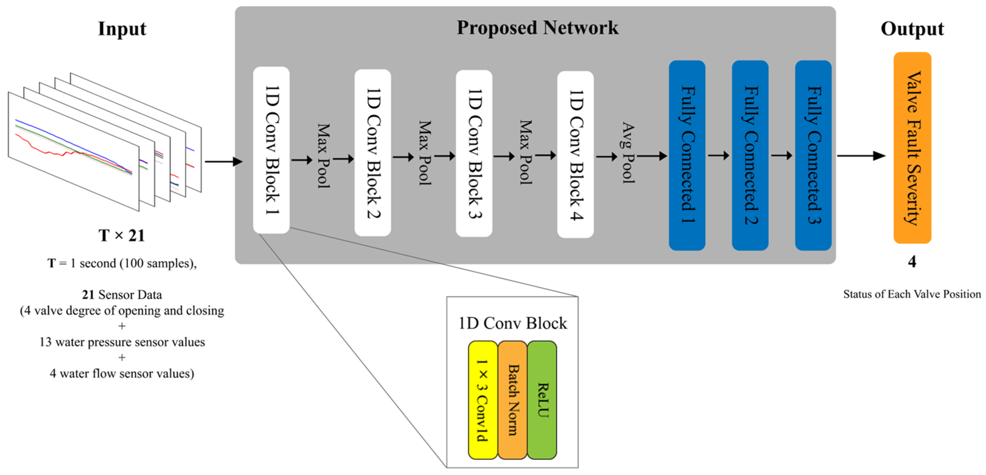
  • Proposed network input composition: This follows the input configuration introduced in the methods section. It consists of the motor rotation values representing the opening and closing amounts of 4 valves, 4 water pressure sensors located at the inlet of each valve, 4 water pressure sensors at the outlet of each valve, a total of 5 water pressure sensors in the main pipe, and a total of 4 flow sensors (a total of 21 input dimensions).
  • Input composition 1: It consists of 4 motor values representing the opening and closing amounts of each valve, 4 water pressure sensors at the inlet of each valve, and 4 water pressure sensors at the outlet of each valve (a total of 12 input dimensions).
  • Input composition 2: It consists of 4 motor values representing the opening and closing amounts of each valve, and only 4 water pressure sensor values at the inlet of each valve (a total of 8 input dimensions).
  • Input composition 3: It consists of 4 motor values representing the opening and closing amounts of each valve, 5 water pressure sensor values located in the main pipe, 4 water pressure sensor values at the inlets of the valves, and 4 water pressure sensor values at the outlets of the valves (a total of 17 input dimensions).
  • Input composition 4: It consists of 4 motor values representing the opening and closing amounts of each valve, 5 water pressure sensor values located in the main pipe, and only 4 water pressure sensor values at the outlet of each valve (a total of 13 input dimensions).
  • Input composition 5: It consists of 4 motor values indicating the opening and closing amounts of each valve, 5 water pressure sensor values, and 4 flow sensor values (a total of 13 input dimensions).
  • Input composition 6: It consists of 4 motor values representing the opening and closing amounts of each valve, and only 4 water pressure sensor values at the outlet of each valve (a total of 8 input dimensions).
  • Input composition 7: It consists of 4 motor values representing the opening and closing amounts of each valve, and only 4 flow sensor values (a total of 8 input dimensions).
  • Input composition 8: It consists of 4 motor values representing the opening and closing amounts of each valve, 5 water pressure sensor values located in the main pipe, and only 4 water pressure sensor values at the inlet of each valve (a total of 13 input dimensions).
  • Input composition 9: It consists of 4 motor values representing the opening and closing amounts of each valve, and only 5 water pressure sensor values located in the main pipe (a total of 9 input dimensions).
As a result, the proposed network input configuration showed the highest accuracy. This is because, even though the four valves are arranged in parallel, a malfunction of one valve affects the other valves as they sequentially receive water from a single main pipe.

5. Conclusions

In this paper, we propose a method for diagnosing valve faults in a multi-valve system consisting of four valves. The system utilizes multivariate time-series data collected from various sensors, including pressure and flow sensors. The data were obtained from an experimental apparatus designed to emulate a multi-valve system where water is sprayed through the valves. The dataset includes state information of the 4 valves collected through 13 pressure sensors and 4 flow sensors. By using the collected data as input to the proposed network, we successfully determined the fault severity of each valve, enabling the identification of both the location and severities of valve faults.
This study specifically introduces a deep learning network capable of simultaneously diagnosing the location and severity of valve faults, thereby enabling the prediction of valve performance degradation. The proposed network accounts for various fault severities likely to occur in real-world environments, making it a robust and effective diagnostic tool for valve faults. Consequently, this enables more efficient operation and management of complex mechanical systems.
The proposed valve fault diagnosis algorithm performed better than traditional methods, including LSTM, FC Layer, RNN, SVM, and RF, in diagnosing valve faults. Furthermore, the proposed method successfully diagnosed fault severities unseen during the training phase, demonstrating its exceptional generalization ability in valve fault diagnosis.
In future studies, we plan to develop a lightweight model for real-time valve state diagnosis. Additionally, we aim to design a network structure capable of diagnosing faults in multiple valves simultaneously within a multi-valve system. Currently, our study focuses on scenarios where a fault occurs in only one of the four valves. However, future research will address cases where multiple faults occur simultaneously across different valves, tackling the increased complexity and interdependence of such scenarios.
Moreover, we are exploring strategies for collecting additional datasets to facilitate the application of the proposed method to larger industrial systems. This includes designing experimental setups that more accurately emulate real-world conditions and integrating sensor configurations tailored to diverse industrial environments. These efforts will ensure the scalability and robustness of the proposed approach in addressing the diagnostic needs of large-scale complex systems.

Author Contributions

E.J.: Conceptualization, Methodology, Software, Data Curation, Writing—Original Draft, and Writing—Review and Editing. J.-H.Y.: Methodology and Software. S.-C.L.: Conceptualization, Supervision, Writing—Review and Editing, Project Administration, and Funding Acquisition. All authors have read and agreed to the published version of the manuscript.

Funding

This research was funded by the development of new products subject to purchase conditions (S3151141) funded by the Ministry of SMEs and Startups (MSS, Korea).

Data Availability Statement

The data will be made available by the authors upon request.

Acknowledgments

The authors sincerely thank Kang-Won Lee and Dong Han Lee for their continuous advice and support throughout this project.

Conflicts of Interest

The authors declare no conflicts of interest.

References

  1. Hu, J.; Yu, Y.; Yang, J.; Jia, H. Research on the generalisation method of diesel engine exhaust valve leakage fault diagnosis based on acoustic emission. Measurement 2023, 210, 112560. [Google Scholar] [CrossRef]
  2. Sim, H.; Ramli, R.; Saifizul, A.; Abdullah, M. Empirical investigation of acoustic emission signals for valve failure identification by using statistical method. Measurement 2014, 58, 165–174. [Google Scholar] [CrossRef]
  3. Navada, B.R.; Sravani, V.; Venkata, S.K. Enhancing Industrial Valve Diagnostics: Comparison of Two Preprocessing Methods on the Performance of a Stiction Detection Method Using an Artificial Neural Network. Appl. Syst. Innov. 2024, 7, 104. [Google Scholar] [CrossRef]
  4. Vashishtha, G.; Chauhan, S.; Sehri, M.; Zimroz, R.; Dumond, P.; Kumar, R.; Gupta, M.K. A roadmap to fault diagnosis of industrial machines via machine learning: A brief review. Measurement 2024, 242, 116216. [Google Scholar] [CrossRef]
  5. Buffa, S.; Fouladfar, M.H.; Franchini, G.; Lozano Gabarre, I.; Andrés Chicote, M. Advanced control and fault detection strategies for district heating and cooling systems—A review. Appl. Sci. 2021, 11, 455. [Google Scholar] [CrossRef]
  6. Vashishtha, G.; Chauhan, S.; Sehri, M.; Hebda-Sobkowicz, J.; Zimroz, R.; Dumond, P.; Kumar, R. Advancing machine fault diagnosis: A detailed examination of convolutional neural networks. Meas. Sci. Technol. 2024, 36, 022001. [Google Scholar] [CrossRef]
  7. Liu, S.; Zhao, T.; Zhang, D. Fault Detection of Flow Control Valves Using Online LightGBM and STL Decomposition. Actuators 2024, 13, 222. [Google Scholar] [CrossRef]
  8. Liang, Q.; Wang, W.; Zhai, Y.; Sun, Y.; Zhang, W. Modeling and Fault Simulation of a New Double-Redundancy Electro-Hydraulic Servo Valve Based on AMESim. Actuators 2023, 12, 417. [Google Scholar] [CrossRef]
  9. Liu, Z.; Yang, X.; Xie, Y.; Wu, M.; Li, Z.; Mu, W.; Liu, G. Multi-sensor cross-domain fault diagnosis method for leakage of ship pipeline valves. Ocean Eng. 2024, 299, 117211. [Google Scholar] [CrossRef]
  10. Yin, H.; Xu, H.; Fan, W.; Sun, F. Fault diagnosis of pressure relief valve based on improved deep Residual Shrinking Network. Measurement 2024, 224, 113752. [Google Scholar] [CrossRef]
  11. Yang, T.; Huang, X.; Zhang, Y.; Li, J.; Zhou, X.; Han, Q. RTCA-Net: A New Framework for Monitoring the Wear Condition of Aero Bearing with a Residual Temporal Network under Special Working Conditions and Its Interpretability. Mathematics 2024, 12, 2687. [Google Scholar] [CrossRef]
  12. Kumar, P.; Khalid, S.; Kim, H.S. Prognostics and health management of rotating machinery of industrial robot with deep learning applications—A review. Mathematics 2023, 11, 3008. [Google Scholar] [CrossRef]
  13. Shi, J.; Yi, J.; Ren, Y.; Li, Y.; Zhong, Q.; Tang, H.; Chen, L. Fault diagnosis in a hydraulic directional valve using a two-stage multi-sensor information fusion. Measurement 2021, 179, 109460. [Google Scholar] [CrossRef]
  14. Hou, Y.; Wang, J.; Chen, Z.; Ma, J.; Li, T. Diagnosisformer: An efficient rolling bearing fault diagnosis method based on improved Transformer. Eng. Appl. Artif. Intell. 2023, 124, 106507. [Google Scholar] [CrossRef]
  15. Tidriri, K.; Chatti, N.; Verron, S.; Tiplica, T. Bridging data-driven and model-based approaches for process fault diagnosis and health monitoring: A review of researches and future challenges. Annu. Rev. Control 2016, 42, 63–81. [Google Scholar] [CrossRef]
  16. Sekunda, A.; Niemann, H.; Poulsen, N.K.; Santos, I. Parametric fault diagnosis of an active gas bearing. Int. J. Control Autom. Syst. 2019, 17, 69–84. [Google Scholar] [CrossRef]
  17. Zhang, S.; Luo, M.; Qian, H.; Liu, L.; Yang, H.; Zhang, Y.; Liu, X.; Xie, Z.; Yang, L.; Zhang, W. A review of valve health diagnosis and assessment: Insights for intelligence maintenance of natural gas pipeline valves in China. Eng. Fail. Anal. 2023, 153, 107581. [Google Scholar] [CrossRef]
  18. Shlezinger, N.; Whang, J.; Eldar, Y.C.; Dimakis, A.G. Model-based deep learning. Proc. IEEE 2023, 111, 465–499. [Google Scholar] [CrossRef]
  19. Wang, T.; Zhang, Q.; Fang, J.; Lai, Z.; Feng, R.; Wei, J. Active fault-tolerant control for the dual-valve hydraulic system with unknown dead-zone. ISA Trans. 2024, 145, 399–411. [Google Scholar] [CrossRef] [PubMed]
  20. Jiang, X.; Xu, X.; Shan, H. Model-Based Fault Diagnosis of Actuators in Electronically Controlled Air Suspension System. World Electr. Veh. J. 2022, 13, 219. [Google Scholar] [CrossRef]
  21. Tian, H.; Li, S.; Gong, Y. Physical Model-based Rapid Quantitative Diagnosis of Solenoid On–Off Valve Spool Stiction Faults. Arab. J. Sci. Eng. 2024, 1–17. [Google Scholar] [CrossRef]
  22. Hu, Z.; Chen, B.; Chen, W.; Tan, D.; Shen, D. Review of model-based and data-driven approaches for leak detection and location in water distribution systems. Water Supply 2021, 21, 3282–3306. [Google Scholar] [CrossRef]
  23. Adedeji, K.B.; Hamam, Y.; Abe, B.T.; Abu-Mahfouz, A.M. Towards achieving a reliable leakage detection and localization algorithm for application in water piping networks: An overview. IEEE Access 2017, 5, 20272–20285. [Google Scholar] [CrossRef]
  24. Chan, T.K.; Chin, C.S.; Zhong, X. Review of current technologies and proposed intelligent methodologies for water distributed network leakage detection. IEEE Access 2018, 6, 78846–78867. [Google Scholar] [CrossRef]
  25. Yin, S.; Li, X.; Gao, H.; Kaynak, O. Data-based techniques focused on modern industry: An overview. IEEE Trans. Ind. Electron. 2014, 62, 657–667. [Google Scholar] [CrossRef]
  26. Ma, D.; Liu, Z.; Gao, Q.; Huang, T. Fault diagnosis of a solenoid valve based on multi-feature fusion. Appl. Sci. 2022, 12, 5904. [Google Scholar] [CrossRef]
  27. Cui, H.; Zhang, L.; Kang, R.; Lan, X. Research on fault diagnosis for reciprocating compressor valve using information entropy and SVM method. J. Loss Prev. Process Ind. 2009, 22, 864–867. [Google Scholar] [CrossRef]
  28. Xiao, S.; Nie, A.; Zhang, Z.; Liu, S.; Song, M.; Zhang, H. Fault diagnosis of a reciprocating compressor air valve based on deep learning. Appl. Sci. 2020, 10, 6596. [Google Scholar] [CrossRef]
  29. Guo, F.-Y.; Zhang, Y.-C.; Wang, Y.; Ren, P.-J.; Wang, P. Fault diagnosis of reciprocating compressor valve based on transfer learning convolutional neural network. Math. Probl. Eng. 2021, 2021, 8891424. [Google Scholar] [CrossRef]
  30. Zhang, X.; Zhang, X.; Liu, J.; Wu, B.; Hu, Y. Graph features dynamic fusion learning driven by multi-head attention for large rotating machinery fault diagnosis with multi-sensor data. Eng. Appl. Artif. Intell. 2023, 125, 106601. [Google Scholar] [CrossRef]
  31. Gálvez, A.; Diez-Olivan, A.; Seneviratne, D.; Galar, D. Fault detection and RUL estimation for railway HVAC systems using a hybrid model-based approach. Sustainability 2021, 13, 6828. [Google Scholar] [CrossRef]
  32. Louen, C.; Ding, S.; Kandler, C. A new framework for remaining useful life estimation using support vector machine classifier. In Proceedings of the 2013 Conference on Control and Fault-Tolerant Systems (SysTol), Nice, France, 9–11 October 2013; pp. 228–233. [Google Scholar]
  33. Lim, R.; Mba, D. Fault detection and remaining useful life estimation using switching Kalman filters. In Engineering Asset Management-Systems, Professional Practices and Certification: Proceedings of the 8th World Congress on Engineering Asset Management (WCEAM 2013) & the 3rd International Conference on Utility Management & Safety (ICUMAS); Springer: Cham, Switzerland, 2015; pp. 53–64. [Google Scholar]
  34. Zhang, K.; Wang, J.; Shi, H.; Zhang, X. A variable working condition rolling bearing fault diagnosis method based on improved triplet loss algorithm. Int. J. Control Autom. Syst. 2023, 21, 1361–1372. [Google Scholar] [CrossRef]
  35. Alabi, A.; Chiesa, M.; Garlisi, C.; Palmisano, G. Advances in anti-scale magnetic water treatment. Environ. Sci. Water Res. Technol. 2015, 1, 408–425. [Google Scholar] [CrossRef]
  36. Dayalan, E.; De Moraes, F.; Shadley, J.R.; Rybicki, E.F.; Shirazi, S.A. CO2 corrosion prediction in pipe flow under FeCO3 scale-forming conditions. In Proceedings of the CORROSION 98, San Diego, CA, USA, 22–27 March 1998; p. NACE-98051. [Google Scholar]
  37. Joshy, N.; Meera, V. Scale control on pipe materials: A review. Green Build. Sustain. Eng. Proc. GBSE 2020, 2019, 421–429. [Google Scholar]
  38. Shaik, N.B.; Pedapati, S.R.; Dzubir, F.A.B. Remaining useful life prediction of a piping system using artificial neural networks: A case study. Ain Shams Eng. J. 2022, 13, 101535. [Google Scholar] [CrossRef]
  39. Rezaei, H.; Ryan, B.; Stoianov, I. Pipe failure analysis and impact of dynamic hydraulic conditions in water supply networks. Procedia Eng. 2015, 119, 253–262. [Google Scholar] [CrossRef]
  40. Cengel, Y.; Cimbala, J. Ebook: Fluid Mechanics Fundamentals and Applications (Si Units); McGraw Hill: New York, NY, USA, 2013. [Google Scholar]
  41. Allamy, S.; Koerich, A.L. 1D CNN architectures for music genre classification. In Proceedings of the 2021 IEEE Symposium Series on Computational Intelligence (SSCI), Orlando, FL, USA, 5–7 December 2021; pp. 1–7. [Google Scholar]
  42. Abrol, V.; Sharma, P. Learning hierarchy aware embedding from raw audio for acoustic scene classification. IEEE/ACM Trans. Audio Speech Lang. Process. 2020, 28, 1964–1973. [Google Scholar] [CrossRef]
  43. Rakhlin, A. Convolutional neural networks for sentence classification. GitHub 2016, 6, 25. [Google Scholar]
  44. Zhang, X.; Zhao, J.; LeCun, Y. Character-level convolutional networks for text classification. In Proceedings of the Advances in Neural Information Processing Systems 28 (NIPS 2015), Montreal, QC, Canada, 7–12 December 2015. [Google Scholar]
  45. Rizvi, S.M.H. Time series deep learning for robust steady-state load parameter estimation using 1D-CNN. Arab. J. Sci. Eng. 2022, 47, 2731–2744. [Google Scholar] [CrossRef]
  46. Tang, W.; Long, G.; Liu, L.; Zhou, T.; Blumenstein, M.; Jiang, J. Omni-scale cnns: A simple and effective kernel size configuration for time series classification. arXiv 2020, arXiv:2002.10061. [Google Scholar]
  47. Riedel, H.; Lorenzen, S.R.; Hübler, C. Object-size-driven design of convolutional neural networks: Virtual axle detection based on raw data. Eng. Appl. Artif. Intell. 2025, 141, 109803. [Google Scholar] [CrossRef]
  48. Krishna, D.; Amrutha, D.; Reddy, S.S.; Acharya, A.; Garapati, P.A.; Triveni, B. Language independent gender identification from raw waveform using multi-scale convolutional neural networks. In Proceedings of the ICASSP 2020—2020 IEEE International Conference on Acoustics, Speech and Signal Processing (ICASSP), Barcelona, Spain, 4–8 May 2020; pp. 6559–6563. [Google Scholar]
  49. Khan, A.; Ko, D.-K.; Lim, S.C.; Kim, H.S. Structural vibration-based classification and prediction of delamination in smart composite laminates using deep learning neural network. Compos. Part B Eng. 2019, 161, 586–594. [Google Scholar] [CrossRef]
  50. Huang, S.; Tang, J.; Dai, J.; Wang, Y. Signal status recognition based on 1DCNN and its feature extraction mechanism analysis. Sensors 2019, 19, 2018. [Google Scholar] [CrossRef] [PubMed]
  51. Lee, K.-W.; Kim, S.-C.; Lim, S.-C. DeepTouch: Enabling touch interaction in underwater environments by learning touch-induced inertial motions. IEEE Sens. J. 2022, 22, 8924–8932. [Google Scholar] [CrossRef]
  52. Kiranyaz, S.; Avci, O.; Abdeljaber, O.; Ince, T.; Gabbouj, M.; Inman, D.J. 1D convolutional neural networks and applications: A survey. Mech. Syst. Signal Process. 2021, 151, 107398. [Google Scholar] [CrossRef]
  53. Cai, X.; Li, D.; Li, F. Enhanced Carbon Price Forecasting Using Extended Sliding Window Decomposition with LSTM and SVR. Mathematics 2024, 12, 3713. [Google Scholar] [CrossRef]
Figure 1. The overall flow of the multi-valve experimental setup includes a pump, 13 pressure sensors, 4 flow sensors, 4 nozzles, 4 motors, 1 main valve, and 4 valves.
Actuators 14 00070 g001
Figure 2. The P&ID of the experimental setup used for dataset collection depicts the locations of the pumps, valves, nozzles, and sensors in the system. In total, 4 valves were arranged in parallel to enable independent operation. A total of 13 water pressure sensors and 4 flow sensors were utilized.
Actuators 14 00070 g002
Figure 3. The images of the experimental setup used for automated valve operation depict the motor-controlled ball valve in three different states: fully open (0°), partially open (45°), and fully closed (90°).
Actuators 14 00070 g003
Figure 4. Illustration of fault severity corresponding to the size of foreign substances inserted into the valve outlet tubes. In the experiment, fault severity was represented based on the size of foreign substances inserted into the tubes connected to the valve outlets: (a) represents the normal valve state, while (be) represent various faulty states.
Actuators 14 00070 g004
Figure 5. Examples of datasets collected through experiments. The sensor data corresponding to the operation of the normal valve and the faulty valve were compared.
Actuators 14 00070 g005
Figure 6. The proposed architecture for diagnosing faults in a multi-valve system using multiple sensors consists of 4 one-dimensional convolutional blocks and 3 fully connected layers. The input has a shape of T × 21, where T represents 100 samples (1 s). The 21 dimensions consist of 13 water pressure sensor values, 4 water flow sensor values, and 4 valve state information.
Actuators 14 00070 g006
Figure 7. Bar graph of the mean difference between the predicted and actual fault severity and the standard deviation of these differences. The length of the bars represents the mean error, while the black error bars represent the standard deviation relative to the mean value.
Actuators 14 00070 g007
Table 1. Fault severity corresponding to the internal diameter of the valve.
Fault SeverityInternal Diameter (mm)
0.07.0
0.15.67
0.24.33
0.33.0
0.42.63
0.52.25
0.61.88
0.71.5
0.81.0
0.90.5
1.00.0
Table 2. Number of valve operation cases.
Number of Operating ValvesCase (Valve Number)
14 cases: (1), (2), (3), and (4)
26 cases: (1, 2), (1, 3), (1, 4), (2, 3), (2, 4), and (3, 4)
34 cases: (1,2,3), (1,2,4), (1,3,4), and (2,3,4)
Table 3. Configuration of the dataset.
Fault SeverityNumber of Operating ValvesNon-Operating
Valve Angle
Training dataset0.0, 0.3, 0.7, 1.01, 2, 323°, 35°, 41°, 47°, 59°
Testing dataset0.0, 0.1, 0.2, 0.3, 0.4, 0.5, 0.6, 0.7, 0.8, 0.9, 1.01, 2, 329°, 53°
Table 4. Proposed network configuration.
Layer NameLayer Description
Input21 × 100
Sensor and motor (valve) angle values over 100 time steps
Convolution 1, Pooling 1Convolution filters 3, Stride 1, Padding 1,
Number of filters 512, Batch normalization,
ReLU, Max pooling 2, Strides 2
Convolution 2, Pooling 2Convolution filters 3, Stride 1, Padding 1,
Number of filters 1024, Batch normalization,
ReLU, Max pooling 2, Strides 2
Convolution 3, Pooling 3Convolution filters 3, Stride 1, Padding 1,
Number of filters 2048, Batch normalization,
ReLU, Max pooling 2, Strides 2
Convolution 4, Pooling 4Convolution filters 3, Stride 1, Padding 1,
Number of filters 4096, Batch normalization,
ReLU, Average pooling 2, Strides 2
Fully ConnectedInput = 24,576, Output = 2048.
Batch normalization, Tanh,
Input = 2048, Output = 1024,
Batch normalization, Tanh,
Input = 1024, Output = 4,
Batch normalization, ReLU
Table 5. Comparison of results for fault severities included in the training dataset, ‘unseen’ fault severities, and the whole dataset.
MAERMSE
Whole case0.03060.0629
Only severities used during training0.00240.0059
Only severities used during testing0.04670.0954
Table 6. Comparison of the MAE and RMSE of the proposed network and other networks in all test fault severities.
MAERMSE
Proposed Network (1D Conv + FC)0.03060.0629
LSTM0.04340.0909
RNN0.08070.1176
FC0.11710.2560
SVM0.24470.3550
RF0.21450.3877
Table 7. Comparison of the MAE and RMSE based on the number of input sensors for the proposed network.
MAERMSE
Proposed network input composition0.03060.0629
Input composition 10.03290.0815
Input composition 20.03590.0899
Input composition 30.03800.1065
Input composition 40.03850.3077
Input composition 50.04420.1115
Input composition 60.04780.1224
Input composition 70.05790.1462
Input composition 80.06400.1333
Input composition 90.12880.3270
Disclaimer/Publisher’s Note: The statements, opinions and data contained in all publications are solely those of the individual author(s) and contributor(s) and not of MDPI and/or the editor(s). MDPI and/or the editor(s) disclaim responsibility for any injury to people or property resulting from any ideas, methods, instructions or products referred to in the content.

