Article

A State Estimation of Dynamic Parameters of Electric Drive Articulated Vehicles Based on the Forgetting Factor of Unscented Kalman Filter with Singular Value Decomposition

1
School of Automotive Engineering, Hubei University of Automotive Technology, Shiyan 442002, China
2
Hubei Key Laboratory of Automotive Power Train and Electronic Control, Hubei University of Automotive Technology, Shiyan 442002, China
3
School of Mathematics, Physics and Optoelectronic Engineering, Hubei University of Automotive Technology, Shiyan 442002, China
*
Author to whom correspondence should be addressed.
Actuators 2025, 14(1), 31; https://doi.org/10.3390/act14010031
Submission received: 27 November 2024 / Revised: 9 January 2025 / Accepted: 13 January 2025 / Published: 15 January 2025
(This article belongs to the Section Actuators for Surface Vehicles)

Abstract

:
In this paper, a state estimation method of distributed electric drive articulated vehicle dynamics parameters based on the forgetting factor unscented Kalman filter with singular value decomposition (SVD-UKF) is proposed. The 7DOF nonlinear dynamics model of a distributed electric drive articulated vehicle is established. The unscented Kalman filter algorithm is the foundation, with singular value decomposition replacing the Cholesky decomposition. A forgetting factor is introduced to dynamically adapt the observation noise covariance matrix in real time, resulting in a centralized parameter state estimator for the articulated vehicle. The proposed parameter state estimation method based on the forgetting factor SVD-UKF is simulated and compared with the unscented Kalman filter (UKF) estimation method. Key dynamic parameters are estimated, such as the lateral and longitudinal velocities and accelerations, angular velocity, articulated angle, wheel speeds, and longitudinal and lateral tire forces of both the front and rear vehicle bodies. The results show that the proposed forgetting factor SVD-UKF method outperforms the traditional UKF method. Furthermore, a prototype vehicle test is conducted to compare the estimated values of various dynamic parameters with the actual values, demonstrating minimal errors. This verifies the effectiveness of the proposed dynamic parameter estimation method for articulated vehicles.

1. Introduction

Articulated vehicles with high mobility, high passability, and high adaptability are widely used in mine development, emergency rescue, agriculture, forestry, and construction [1,2]. During the traveling process of articulated vehicles, obtaining the key dynamic parameters of the vehicle is the basis for the safe operation and stability control of the vehicle. However, some dynamic parameters are difficult to measure, and sensors are expensive, increasing the actual production cost of articulated vehicles. On the other hand, low-cost sensors tend to have high measurement noise and poor accuracy, necessitating parameter state estimation methods [3,4,5]. Due to the special configuration of articulated vehicles, dynamic models of articulated vehicles have more nonlinearities and more governing parameters, which increase the difficulty of estimating the dynamic parameters of articulated vehicles. Therefore, the study of state estimation methods for kinetic parameters of articulated vehicles has important theoretical and engineering values.
For vehicle state parameter estimation, the main methods are model-based estimation methods and data-based estimation methods. Model-based methods involve establishing vehicle kinematic or dynamic models and using techniques such as least squares, Kalman filtering, sliding mode, robust estimation, and fuzzy estimation [6,7,8]. Fusing and filtering multi-sensor measurements require accurate vehicle modeling and consideration of uncertainties and disturbance terms. Data-based methods utilize neural networks, machine learning, and other methods [9,10] to build data-driven models using a large amount of experimental data. These methods do not depend on a kinetic model but require a large amount of high-quality training data. The convergence calculation speed is slow, and the generalization is poor. Regarding the whole structure of vehicle state parameter estimation, the methods are mainly divided into centralized estimation methods [11] and modular estimation methods [12]. Centralized estimation methods are relatively straightforward but demand highly accurate dynamic models, which increase the complexity of both the vehicle model and the estimation model when the number of estimated parameters is large. The main method is relatively more flexible, and different methods can be used for estimation according to different states. The estimation structure is complex, with early results significantly influencing later stages, potentially overlooking the nonlinear coupling effects between different estimation phases.
Among the common estimation methods, the least squares method has the problem of data saturation. The sliding mode algorithm easily produces jitter, the robust estimation of the optimum is poor, and it is more difficult to establish complete fuzzy rules with fuzzy estimation. In contrast, the Kalman filter and its variants demonstrate better adaptability to nonlinear systems, offering relatively stable estimation performance and superior accuracy [13]. H. Ahmadi applied an extended Kalman filter to estimate the dynamic state parameters of a heavy articulated trailer, such as the lateral and longitudinal velocities, yaw rate, and articulated angle, and conducted simulations on both dry and wet road surfaces to validate the approach [14]. Zygimantas designed an extended Kalman filter to estimate the articulated angle and truck steering angle as inputs to the system and validated it using real vehicles [15]. H. Sah proposed two methods for estimating EKF noise parameters—particle swarm optimization (PSO) and gradient-based optimization—and applied EKF to estimate the steering angle, articulated angle, and the lateral and longitudinal tire forces of a tractor-semitrailer [16]. Wang Wenwei developed a 3-DOF linear dynamic model and employed particle filter theory to estimate the state variables of an articulated bus, including the yaw rate, articulation rate, articulated angular velocity, and articulated angle of the front vehicle body [17]. Gao Lulu estimated the road adhesion coefficient of an electric drive articulated vehicle by using the least squares method with a forgetting factor and estimated the vehicle-related state parameters using Kalman filtering [18]. Cheng used H∞ filtering and Kalman filtering to jointly estimate the state parameters and vehicle center of mass position of a multi-axle wheel side electric drive articulated bus and compared and analyzed the estimation effects of EKF and UKF [19]. Yang applied an improved square root UKF to estimate the tire force and center of mass position of articulated vehicles [20]. Gao employed a strong tracking algorithm in UKF to rapidly estimate vehicle tire forces [21].
In this paper, a 7DOF nonlinear dynamics model of distributed electric drive articulated vehicles is established. In contrast to previous research on the state estimation of articulated vehicles, this paper establishes a centralized state estimator that contains the dynamic parameters of the front and rear vehicle bodies in the lateral, longitudinal, and yaw directions, as well as the articulated angle, wheel speed, and the tire force. This prevents early results from influencing later stages, and the estimator structure is more simplified. In order to improve the estimation convergence, we employ the UKF algorithm, utilizing SVD to address the challenge of non-positive definiteness in the covariance matrix. The convergence and accuracy of estimation are further improved by introducing a forgetting factor, which increases the weight of more recent data. With this centralized estimator and the proposed SVD-UKF with the forgetting factor estimation method, the convergence and accuracy of the estimator can be improved in different environments and noises.
In Section 2, we develop a seven-degree-of-freedom (7DOF) nonlinear dynamics model for the articulated vehicle. Section 3 provides a detailed description of the proposed SVD-UKF parameter estimation method, including the relevant system state equations and observation equations. The validation of the estimation algorithm through simulation is thoroughly discussed in Section 4, where we also conduct a comparative analysis with the UKF. In Section 5, the proposed estimation method is experimentally validated using a prototype vehicle. Finally, we conclude the paper with a comprehensive discussion of our findings and their implications for future research.

2. Nonlinear Dynamics Modeling of Articulated Vehicles

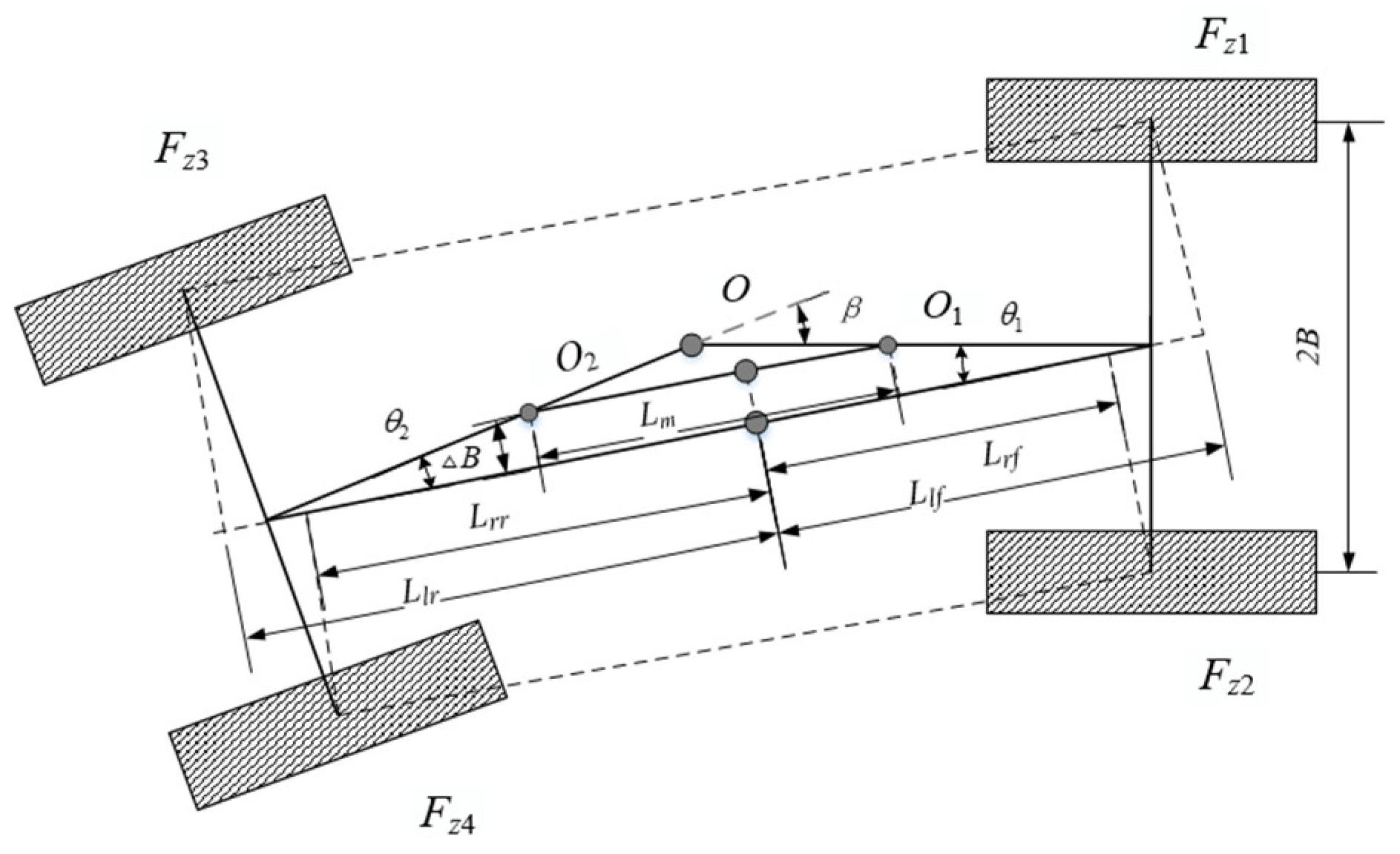
The articulated vehicle dynamics model is the research basis for the state estimation of dynamics parameters, and a 7DOF nonlinear dynamics model of distributed electric drive articulated vehicles is established. The dynamics model is shown in Figure 1, and the related quantities applied in this paper are in the nomenclature. The model is planar, representing a relatively slow articulated vehicle. The focus is on the lateral, longitudinal, and yaw degrees of freedom of the front and rear bodies, while the vertical, roll, and pitch degrees of freedom are neglected. A force analysis of the articulated vehicle is carried out to obtain the equilibrium equations for the lateral, longitudinal, and yaw of the front and rear vehicle bodies. Specific dynamics analysis and modeling details can be found in a previous study [22]. The articulated vehicle dynamics model is simplified as follows: (1) The front and rear body centers are located on the longitudinal central axis, and the vehicle is symmetrical with respect to the longitudinal central axis. (2) The influence of the tire camber angle and return torque on wheel dynamics is neglected. (3) Air resistance is ignored, and the road surface is flat and two-dimensional.
The articulated vehicle dynamics equations are shown in Equation (1). The initial Newtonian mechanics equations and the simplification process are shown in Appendix A.
m 1 + m 2 v ˙ x 1 = m 2 + m 1 w 1 v y 1 + m 2 L 4 w ˙ 2 sin β m 2 L 2 w 1 2 m 2 L 4 w 2 2 cos β + F x 1 + F x 2 + F x 3 + F x 4 cos β + F y 3 + F y 4 sin β m 1 + m 2 v ˙ y 1 = m 2 L 2 w ˙ 1 m 1 + m 2 w 1 v x 1 + m 2 L 4 w ˙ 2 cos β + m 2 L 4 w 2 2 sin β + F y 1 + F y 2 + F y 3 + F y 4 cos β F x 3 + F x 4 sin β I 1 w ˙ 1 = M O 1 + ( F x 1 F x 2 ) B + ( F y 1 + F y 2 ) L 1 + L 2 m 1 v ˙ y 1 + v x 1 ω 1 L 2 I 2 ω ˙ 2 = M O 2 + ( F x 3 F x 4 ) B ( F y 3 + F y 4 ) L 3 + F y 1 + F y 2 L 4 cos β + F x 1 + F x 2 L 4 sin β m 1 v ˙ y 1 + v x 1 ω 1 L 4 cos β m 1 v ˙ x 1 v y 1 ω 1 L 4 sin β
During the vehicle’s traveling, each wheel’s vertical load will change with the articulated angle and acceleration changes. The analysis of each wheel’s vertical load is shown in Figure 2. Due to the unique steering characteristics of articulated vehicles, the center of mass position can be calculated based on relevant vehicle parameters, allowing for the subsequent calculation of the vertical loads on each wheel, as shown in Equation (2). The detailed calculation process is provided in Appendix A.
F z 1 = L l r L l f + L l r B cos θ 2 + Δ B 2 B cos θ 2 m 1 + m 2 g B cos θ 2 + Δ B m 1 + m 2 a x h 2 B L cos θ 2 + L l r L l f + L l r m 1 + m 2 a y h 2 B cos θ 2 F z 2 = L r r L r f + L r r B cos θ 2 Δ B 2 B cos θ 2 m 1 + m 2 g B cos θ 2 Δ B m 1 + m 2 a x h 2 B L cos θ 2 L r r L r f + L r r m 1 + m 2 a y h 2 B cos θ 2 F z 3 = L l f L l f + L l r B cos θ 2 + Δ B 2 B cos θ 2 m 1 + m 2 g + B cos θ 2 + Δ B m 1 + m 2 a x h 2 B L cos θ 2 + L l f L l f + L l r m 1 + m 2 a y h 2 B cos θ 2 F z 4 = L r f L r f + L r r B cos θ 2 Δ B 2 B cos θ 2 m 1 + m 2 g + B cos θ 2 Δ B m 1 + m 2 a x h 2 B L cos θ 2 L r f L r f + L r r m 1 + m 2 a y h 2 B cos θ 2
In this paper, the Dugoff tire model is used, which provides a method for calculating the forces under the combined action of lateral and longitudinal forces [23]. It is characterized by a fast calculation speed, and the lateral and longitudinal forces of the tire can be obtained from the vertical force of the tire, the side slip angle of the tire, and the longitudinal slip rate during the calculation. The model equations are as follows:
F x = C σ S t i 1 + S t i f ( λ ) F y = C α tan ( α ) 1 + S t i f ( λ )
where λ = μ F z 1 + S t i 2 C σ S t i 2 + C σ tan ( α ) 2 1 / 2 f ( λ ) = ( 2 λ ) λ   λ < 1 1   λ 1 . The other parameters and the calculation process are described in Appendix B.

3. Adaptive Forgetting Factor SVD-UKF Articulated Vehicle Dynamics Parameter Estimation

3.1. Adaptive Forgetting Factor SVD-UKF(ASVD-UKF)

The equations of state and observation for a nonlinear discrete system are as follows:
X k + 1 = f ( x ( k ) ) + w ( k ) Z k = h ( x ( k ) ) + v ( k )
where X k + 1   is the state of the system at a moment, f ( x ( k ) ) is the nonlinear equation of state, Z k is the measured value of the system at time k , h ( x ( k ) ) is the nonlinear observation equation, and w ( k ) and v ( k ) are the zero mean and uncorrelated white noise.
The specific procedure for calculating the UKF for this system at different moments, k, are as follows.
The first step is to obtain the sampling points (Sigma points) and weights. Through the unscented transformation, 2n + 1 Sigma points and the corresponding weights can be obtained, i.e., sample point χ and weight ω   , and n is the dimension of the state. The calculation process is as follows:
χ ( 0 ) = x ̄ , i = 0 χ ( i ) = x ̄ + ( n + λ ) P , i = 1 : n χ ( i ) = x ̄ ( n + λ ) P , i = n + 1 : 2 n
where x is the n-dimensional state variable; x ̄ and P are the mean and covariance of x , respectively. The weights of these sampling points are calculated as follows:
ω ( 0 ) m = λ n + λ ω ( 0 ) c = λ n + λ + 1 α 2 + ζ ω ( i ) m = ω ( i ) c = 1 2 ( n + λ ) , i = 1 : 2 n
where the superscript m is the mean, c is the covariance, λ = α 2 ( n + κ ) n , and λ is the scaling factor, which reduces the prediction error. The value of α can control the distribution state of the sampling points; the parameter κ is chosen by oneself, and it should be noted that it is usually ensured that the matrix n + λ P is a semi-positive definite matrix.
χ ( i ) ( k k ) = [ x ^ ( k k ) , x ^ ( k k ) + ( n + λ ) P ( k k ) , x ^ ( k k ) ( n + λ ) P ( k k ) ]
In the second step, the prediction is estimated for 2n + 1 Sigma points.
χ ( i ) ( k + 1 k ) = f k , χ ( k k )
In the third step, the prediction estimates and covariances of the new Sigma points are weighted.
x ^ k + 1 k = i = 0 2 n ω ( i ) m χ ( i ) k + 1 k
P k + 1 k = i = 0 2 n ω ( i ) c x ^ k + 1 k χ ( i ) k + 1 k x ^ k + 1 k χ ( i ) k + 1 k T + Q
where Q is the process noise covariance matrix.
In the fourth step, the unscented transformation is applied once again to calculate the new set of sampling points.
χ ( i ) ( k + 1 k ) = [ x ^ ( k + 1 k ) , x ^ ( k + 1 k ) + ( n + λ ) P ( k + 1 k ) , x ^ ( k + 1 k ) ( n + λ ) P ( k + 1 k )
In the fifth step, the set of points obtained from the calculation in the fourth step is carried over to the observation equation to obtain the prediction observations.
Z ( i ) ( k + 1 k ) = h χ ( i ) ( k + 1 k )
In the sixth step, the set of points of the prediction measurements calculated in the fifth step is weighted and summed to obtain the mean and covariance of the system prediction.
Z ̄ ( k + 1 k ) = i = 0 2 n ω ( i ) Z ( i ) ( k + 1 k )
P z k z k = i = 0 2 n ω ( i ) Z ( i ) ( k + 1 k ) Z ̄ ( k + 1 k ) Z ( i ) ( k + 1 k ) Z ̄ ( k + 1 k ) T + R
where R is the observation noise.
P x k z k = i = 0 2 n ω ( i ) X ( i ) ( k + 1 k ) Z ̄ ( k + 1 k ) Z ( i ) ( k + 1 k ) Z ̄ ( k + 1 k ) T
In the seventh step, the Kalman gain matrix is calculated to calculate the system state update and covariance update.
K ( k + 1 ) = P x k z k P z k z k 1
X ^ ( k + 1 k + 1 ) = X ^ ( k + 1 k ) + K ( k + 1 ) [ Z ( k + 1 ) Z ^ ( k + 1 k ) ]
P ( k + 1 k + 1 ) = P ( k + 1 k ) K ( k + 1 ) P z k z k K T ( k + 1 )
In UKF estimation, Cholesky decomposition is typically used to handle the covariance matrix, and it is required to be a positive definite matrix. However, in practical applications, due to observation errors and nonlinearity, it is challenging to ensure the positive definiteness of the covariance matrix, leading to decreased filter accuracy or even divergence. SVD does not require the matrix to be positive and definite and offers high accuracy and speed. Therefore, SVD decomposition is used instead of Cholesky decomposition. During the unscented transformation process, the computation of sampling points based on SVD decomposition is carried out as follows:
P = U Λ V T = U S 0 0 0 V T
χ ( 0 ) = x ̄ , i = 0 χ ( i ) = x ̄ + ( n + λ ) U Λ , i = 1 : n χ ( i ) = x ̄ ( n + λ ) U Λ , i = n + 1 : 2 n
In actual vehicle parameter state estimation, due to simplification in the process of establishing the vehicle dynamics model, the model error caused by the vehicle’s inherent high nonlinearity, and the measurement error caused by external interference in the process of sensor measurement, the estimation accuracy and convergence will be affected. The UKF is an infinite memory filter, which utilizes data from the previous estimation process in each update iteration. As the number of iterations increases, there is a larger proportion of historical data and a smaller proportion of recent data. Consequently, the corrective effect of new observation data on state estimation weakens, leading to poor suppression of estimation errors, causing error accumulation and potentially resulting in divergence. In addition, in the actual work of articulated vehicles, the environment is harsh, the working conditions are complicated, and measurement noise is easily interfered with by external uncertainties, which will lead to the reduction in estimation accuracy if it is taken as a constant value.
To solve the above problems, it is necessary to increase the proportion of recent data and reduce the proportion of historical data. In this paper, a forgetting factor is introduced to adjust the observation noise covariance matrix R dynamically in real time so as to improve the convergence of the estimation and the estimation accuracy. The noise covariance matrix R is calculated as
R k + 1 = 1 d k R k + d k × e k e k T i = 0 2 n ω ( i ) c Z k + 1 Z ̄ k + 1 Z k + 1 Z ̄ k + 1 T
where e k is the residual, b is the forgetting factor, and b takes a value in the range of 0–1, though it usually takes a value in the range of 0.9–0.99. The forgetting factor increases the weight of recent data while gradually “forgetting” older data. Reducing the value of the forgetting factor enhances the memory of historical data, thereby improving the stability of the model. Conversely, increasing the value of the forgetting factor allows for quicker adaptation to new data, thus enhancing the sensitivity. To prevent the estimator from being overly sensitive to the selection of the forgetting factor, this paper employs a weighted exponential decay method d k to ensure robustness. The parameters d k , e k , and d k are calculated as follows:
e k = Z k + 1 Z ̄ k + 1
d k = 1 b 1 b k
The flowchart of the SVD-UKF estimation method is shown in Figure 3.

3.2. System State Equations and Observation Equations

According to the research content of the paper, combined with the state estimation dynamics model, the key state estimation parameters of the articulated vehicle include lateral and longitudinal velocities, lateral and longitudinal accelerations, angular velocities, the articulated angle of the front and rear vehicle bodies, wheel speeds, and longitudinal and lateral forces of the tires, so the system state variables are
x ( k ) = v x 1   v y 1   a x 1   a y 1   ω 1   v x 2   v y 2   a x 2   a y 2   ω 2   β   ω t 1   ω t 2   ω t 3   ω t 4   F x 1   F x 2   F x 3   F x 4   F y 1   F y 2   F y 3   F y 4 T
Since the system is discrete, iterative computation is required for the before and after moments. The system state equation can be obtained as Equation (25). Detailed formulas are shown in Appendix C.
x i ( k + 1 ) = x i ( k ) + f i Δ t + w i ( k )
Using the IMU and other sensors, the acceleration, the angular velocity of the articulated angle, and the wheel speed can be measured, so the observed quantities are
z ( k ) = a x 1   a y 1   ω 1   a x 2   a y 2   ω 2   β   ω t 1   ω t 2   ω t 3   ω t 4 T
The observation equations are
z i ( k + 1 ) = H x i ( k + 1 ) + v i ( k + 1 )
The observation matrix H is
H = h 1 h 2 h 22 h 23
For which parameter h = 0 when i = 1 , 2 , 6 , 7 , 16 , 17 , 18 , 19 , 20 , 21 , 22 , 23 , and b = 1.
Due to the electric drive and the corresponding sensors, the steering torque of the articulated vehicle and the wheel drive torque can be used as input parameters of the system, and the input state parameters of the system are
u = M O   T t 1   T t 2   T t 3   T t 4

4. Simulation Analysis

Based on the nonlinear dynamics model of the articulated vehicle constructed in the paper, the parameter estimation method constructed in Section 3 is simulated and analyzed. The UKF estimation method and the ASVD-UKF estimation method are, respectively, utilized for parameter simulation estimation, and the estimation effects of the two estimation algorithms are compared and analyzed.

4.1. Simulation Settings

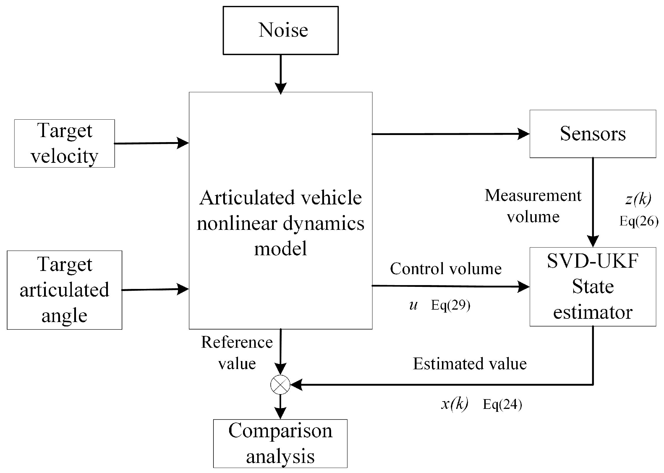
The target longitudinal velocity and articulated angle of the front vehicle body are used as target inputs, as shown in Figure 4. Each dynamic parameter of the vehicle obtained from the nonlinear dynamics model of the articulated vehicle is used as the reference value of each estimator in the simulation verification, the measured value of the state estimator is used for the mesoscopic measurement, and the whole simulation verification process is shown in Figure 5.

4.2. Analysis of Simulation Results

In evaluating the effectiveness of vehicle parameter estimation, metrics such as the mean absolute error (MAE) and root mean square error (RMSE) are commonly used for quantitative assessment. However, the MAE and root mean square error (RMSE) are absolute measures, which are not obvious for different physical quantities as well as values of different magnitudes, especially the relative error. The mean absolute percentage error (MAPE), as a relative error metric, avoids the cancelation of positive and negative errors, providing a better representation of the relative error between the estimated and true values and expressing the error in percentage terms. The MAPE is calculated as follows:
MAPE = 100 % n i = 1 n x i _ r x i _ e x i _ r
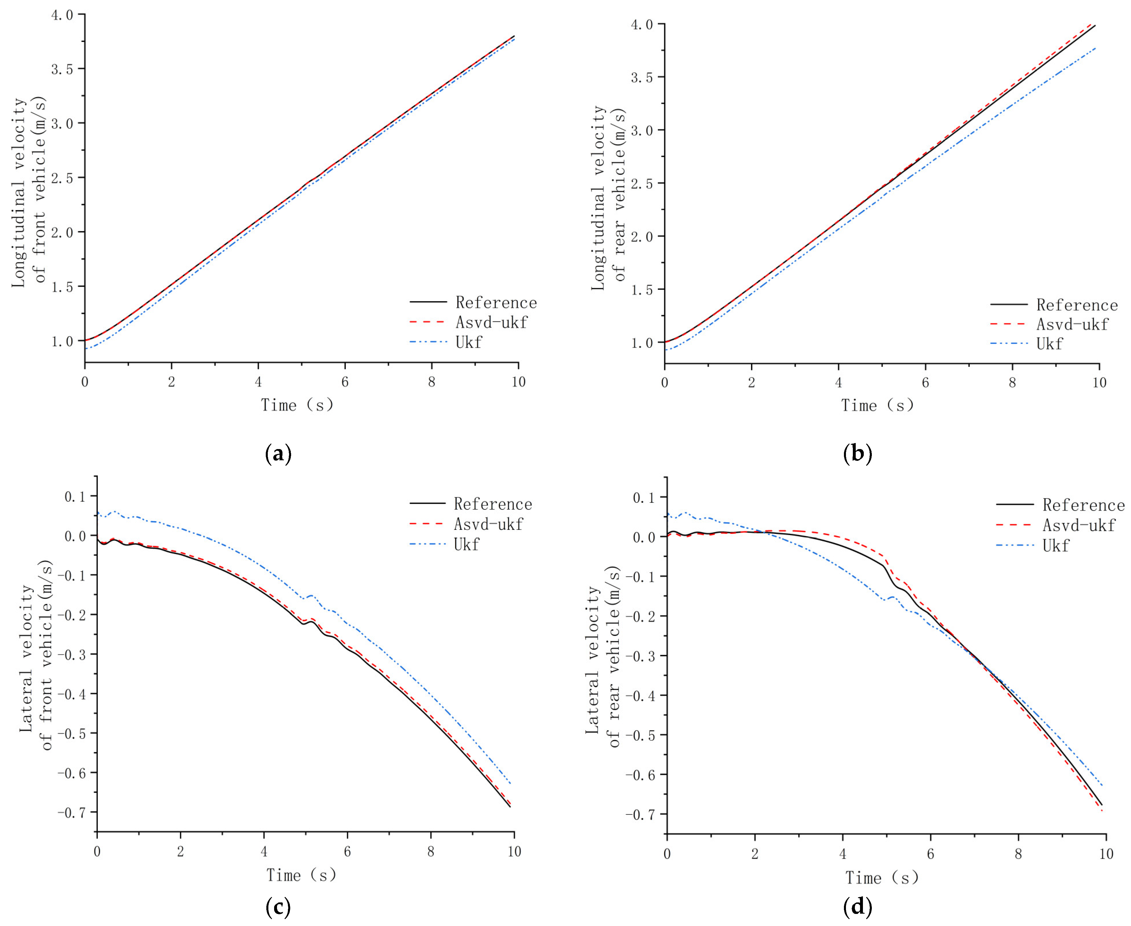
Figure 6 shows the estimation results of the longitudinal and lateral velocities of the front and rear bodies of the articulated vehicle. Overall, the ASVD-UKF estimation method is more accurate than the UKF method. The longitudinal velocity estimation of the front vehicle body is slightly better than the rear vehicle estimation. The MAPE values of the estimated and reference values of the longitudinal and lateral velocities of the front and rear vehicle bodies are 0.63%, 0.48%, 1.25%, and 1.87%, respectively, while the MAPE values of the UKF estimates and reference values are 2.46%, 8.60%, 5.15%, and 3.73%. The ASVD-UKF estimation has a smaller error, and the estimation is better both in terms of estimation accuracy and estimation convergence.
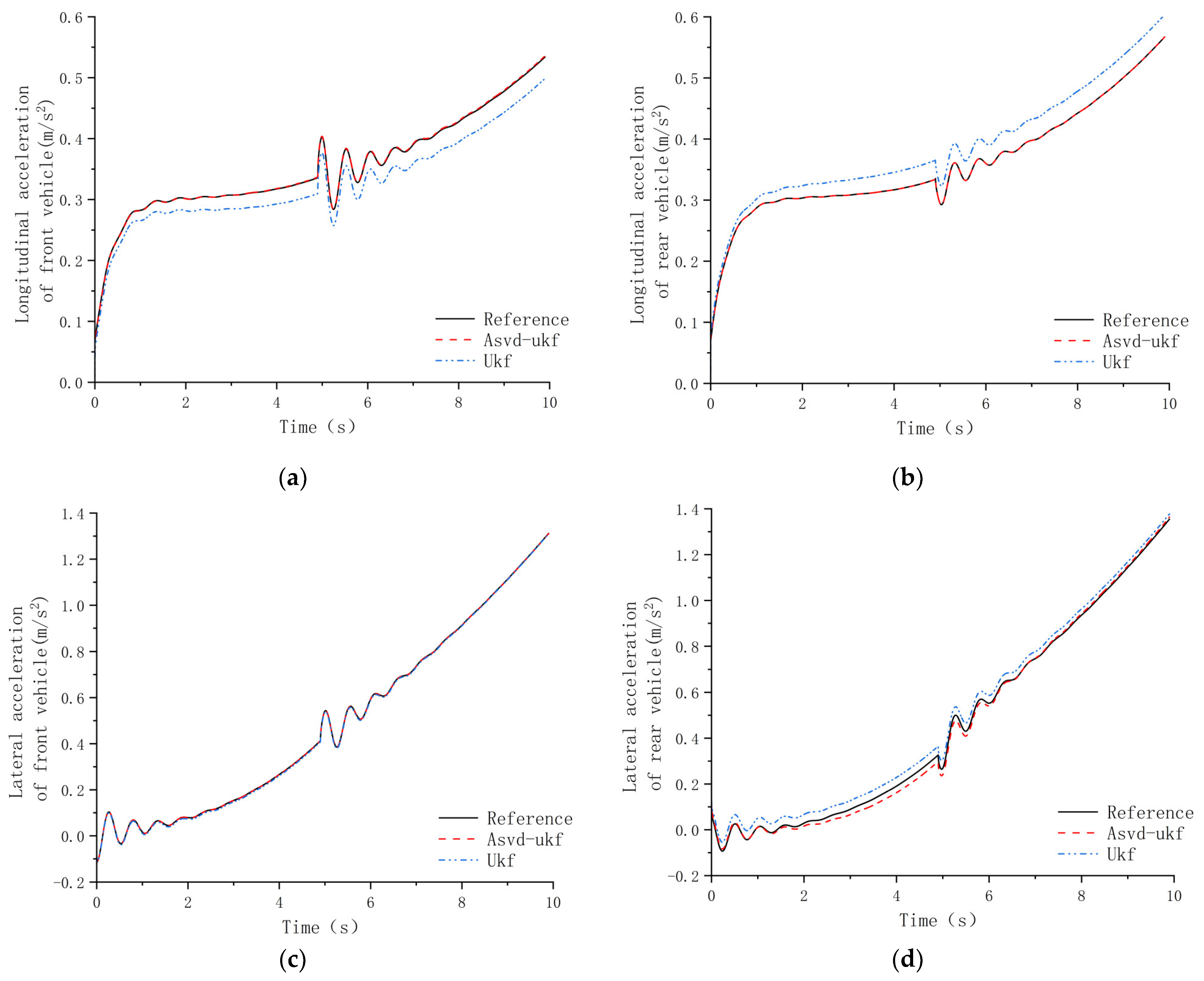
The results of the longitudinal and lateral acceleration estimations of the front and rear vehicle bodies are shown in Figure 7. The estimated values of ASVD-UKF and the reference value MAPE are, respectively, 1.16%, 1.14%, 1.66%, and 1.89%. The differences in errors between the front and rear bodies are minimal. As the velocity increases, the accelerations of both the front and rear bodies gradually increase. At 5 s, due to the constant articulated angle, the front and rear bodies exhibit opposite fluctuation trends. The MAPE values of the UKF estimation and the reference value are 7.50%, 7.20%, 1.92%, and 2.41%. The UKF method shows larger errors in longitudinal acceleration estimation, while the lateral acceleration estimates are relatively closer to those of the ASVD-UKF method.
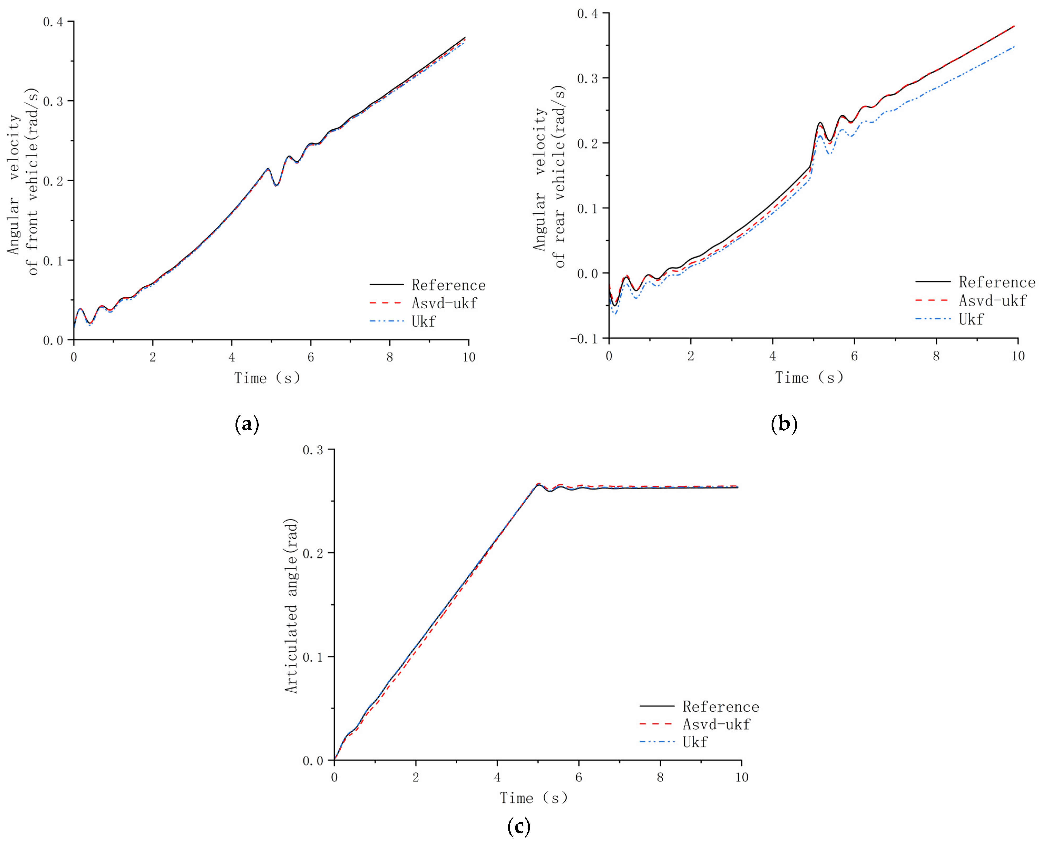
Figure 8 shows the angular velocity and articulated angle of the front and rear vehicle bodies of the articulated vehicle. Overall, both methods yield similar estimation results for the front vehicle angular velocity and articulated angle. In the estimation of the angular velocity of the rear vehicle body, the estimation of ASVD-UKF is slightly better than that of UKF. The estimated and reference MAPE values of ASVD-UKF are 2.58%, 2.69%, and 2.98%, while the estimated and reference values MAPE for UKF are 2.85%, 3.37%, and 1.20%. Due to the articulated steering form, during the gradual increase in the articulated angle, the angular velocity of the front and rear vehicle bodies at the initial moment has the opposite trend, and the estimated values of the front and rear vehicle bodies are also gradually stabilized after the articulated angle is kept constant.
Figure 9 shows the rotational speeds of each wheel of the articulated vehicle. As the number of wheels increases, the wheel speeds also increase. Due to the continuous steering of the vehicle, the wheel speeds on either side differ slightly, with tire 1 and tire 3 having higher speeds than tire 2 and tire 4. At 5 s, the wheel speed fluctuates slightly because the articulated angle remains constant, but the overall speed remains stable. The estimation results from both methods show minimal errors compared to the reference values, indicating close estimation results and good tracking performance.
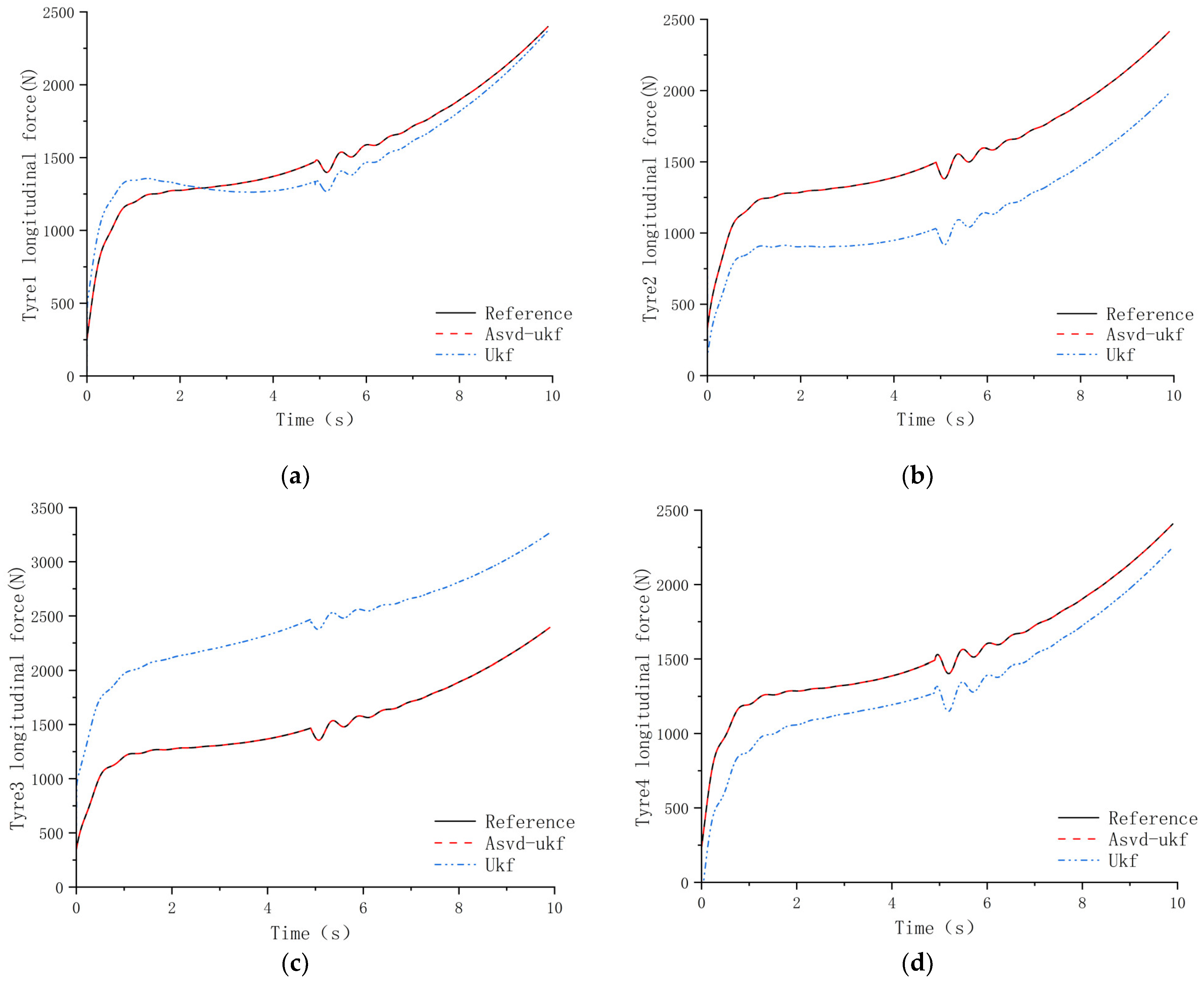
The estimated longitudinal tire force of each tire of the articulated vehicle is shown in Figure 10. With the increase in velocity and acceleration, the tire longitudinal force increases gradually and has a similar trend. Overall, the ASVD-UKF estimation is better than the UKF estimation in terms of estimation error and convergence. The MAPE values for the ASVD-UKF are 0.08%, 0.10%, 0.20%, and 0.14%. In contrast, the UKF method shows relatively better performance for tires 1 and 4, while tires 2 and 3 have larger estimation errors and poorer convergence, with MAPE values of 7.45%, 27.6%, 61.3%, and 16.23%.
The lateral force of each tire of the articulated vehicle is shown in Figure 11. As the vehicle velocity and articulated angle increase, the lateral force of each tire gradually increases. The rear vehicle lateral force estimates have a larger error than the front vehicle body’s lateral force during steering. Although the ASVD-UKF estimation is still better than the UKF estimation, the difference between the two estimation results is smaller than the longitudinal force. The MAPE values of the ASVD-UKF estimates to the reference values are 3.63%, 3.88%, 4.41%, and 4.27%. The MAPE values of the UKF estimates to the reference values are 10.6%, 10.9%, 8.74%, and 13.4%.

5. Experimental Verification

Following a comprehensive simulation analysis, the effectiveness of the proposed ASVD-UKF estimation method has been thoroughly validated. The results demonstrate that the ASVD-UKF method significantly outperforms the conventional UKF method in terms of estimation accuracy. In this section, we provide additional validation of the estimation performance through a series of experimental tests conducted on a prototype vehicle.

5.1. Distributed Electric Drive Principle Prototype Vehicle and Test Program

In this study, we perform a detailed analysis of the motion forms, system structure, and drive force modes of distributed electric drive articulated vehicles. Based on the principle of similarity, we establish an experimental prototype vehicle that closely resembles the actual vehicle. The drive wheels are selected to be hub motors with torque and speed sensors. The steering part includes an electric actuator and linear displacement sensor, which can measure the displacement change and calculate the change in articulated angle. The electric actuator coaxial arrangement of the tensile force sensor can measure the entire steering system of the tensile force. The vehicle was controlled using a laptop equipped with a 12th-generation Core i7 processor, which provided sufficient computational power to facilitate real-time acquisition and storage of sensor signals. This configuration ensured that the system could effectively manage the complex data processing requirements necessary for the successful operation of the vehicle. The whole test principle prototype is shown in Figure 12.
Through the inertial measurement units (IMUs) on the front and rear vehicle bodies of the test principle prototype vehicle, the longitudinal acceleration, lateral acceleration, and angular velocity of the front and rear vehicle bodies can be obtained. The IMUs are automotive-grade Bosch IMUs. The acquisition accuracy is 0.01 degrees to ensure the accuracy of the acquired data. Using displacement and force sensors in the steering system, we can calculate the articulated angle and the steering torque. The wheel speed and driving torque are acquired through feedback from the hub motors. The obtained quantities are brought into the estimator as control inputs and observations of the state estimation method to estimate the key vehicle dynamics parameters. The lateral and longitudinal velocities of the front vehicle body can be acquired by real-time kinematics (RTK), and the measured values of each kinetic parameter obtained from each sensor are taken as the real values to validate the state estimation method, as shown in Figure 13. In the whole driving process, the articulated test principle prototype vehicle at a certain speed first carried out a period of straight-line driving and then entered the steering state, and it finally carried out slewing movement at a certain angle.
The information related to the sensors used during the experiment is shown in Table 1.

5.2. Analysis of Test Results

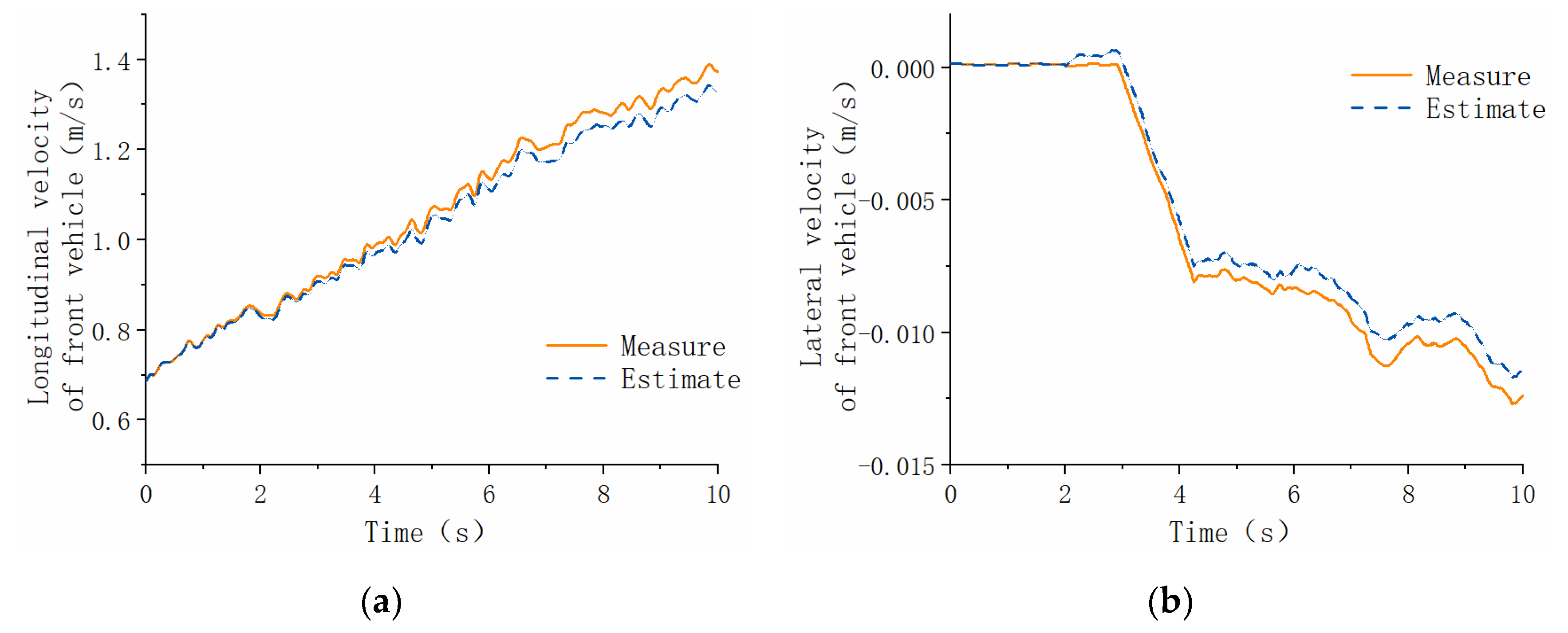
The longitudinal and lateral velocities of the front body of the articulated vehicle are shown in Figure 14. During the first 3 s of travel, the vehicle remains in a straight-line state, resulting in a near-zero lateral speed, while the longitudinal velocity is in the acceleration phase. By comparing the true values with the estimated values, it can be observed that the overall estimations of the longitudinal and lateral velocities of the front vehicle body are quite accurate. The MAPE values between the measured values and the estimated values are 1.30% and 3.61%, respectively, indicating a small error. Compared to the true values, the estimated values exhibit good tracking performance, though the estimated lateral speed is slightly smaller than the measured value.
The angular velocity curves of the front and rear vehicle bodies are shown in Figure 15. During straight-line driving, both the estimated values and the measured values remain close to the zero line. During the steering process, the angular velocity of the rear vehicle body exhibits a noticeable lag, but the estimated values still closely follow the actual changes. In the process of traveling at a fixed angle, due to the influence of speed and road surface, the estimated value of the front and rear vehicle bodies has some fluctuation with the measured value, and the MAPE values of the two are 6.16% and 4.21%, respectively. The estimation error is small and has a good following, and the estimated value of the rear body’s angular velocity is slightly larger than the measured value. The articulated angle has a good estimation of the estimated value during straight-line driving, steering, and fixed-angle slewing, with an MAPE of 1.54% between the estimated value and the measured value.
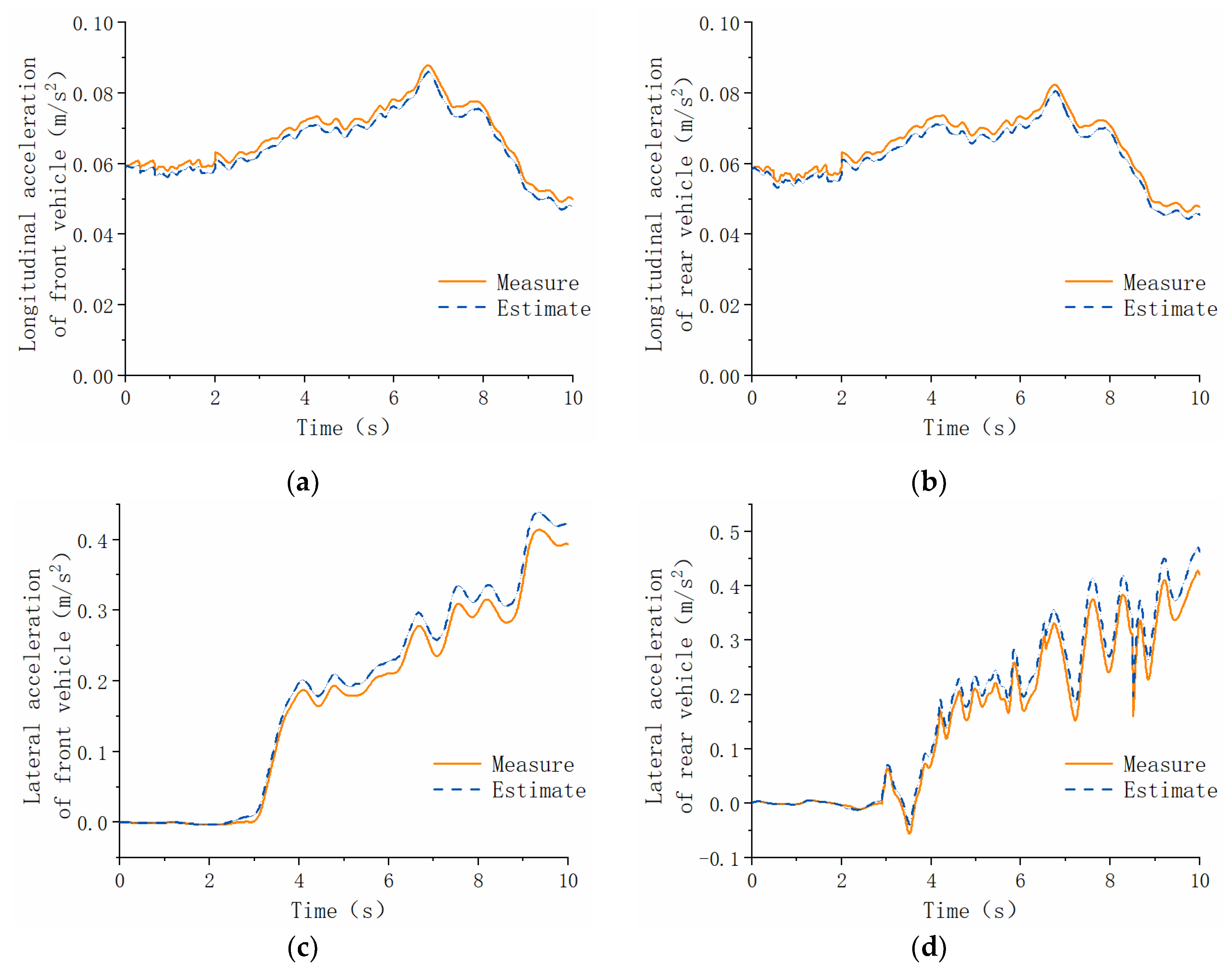
The longitudinal and lateral acceleration curves of the front and rear vehicle bodies are shown in Figure 16. The longitudinal acceleration of the front and rear vehicle bodies is better estimated, and the measured value and estimated MAPE value are 2.07% and 2.25%, indicating minimal error. However, the estimation error for the lateral acceleration is slightly larger compared to the longitudinal acceleration, with MAPE values of 6.43% and 3.31% for the measured and estimated values. During steering and slewing, the rear body has a relative lagging tendency, and the lateral acceleration of the rear body changes more drastically. The estimated longitudinal acceleration is slightly smaller than the measured value, while the estimated lateral acceleration is slightly larger than the measured value.
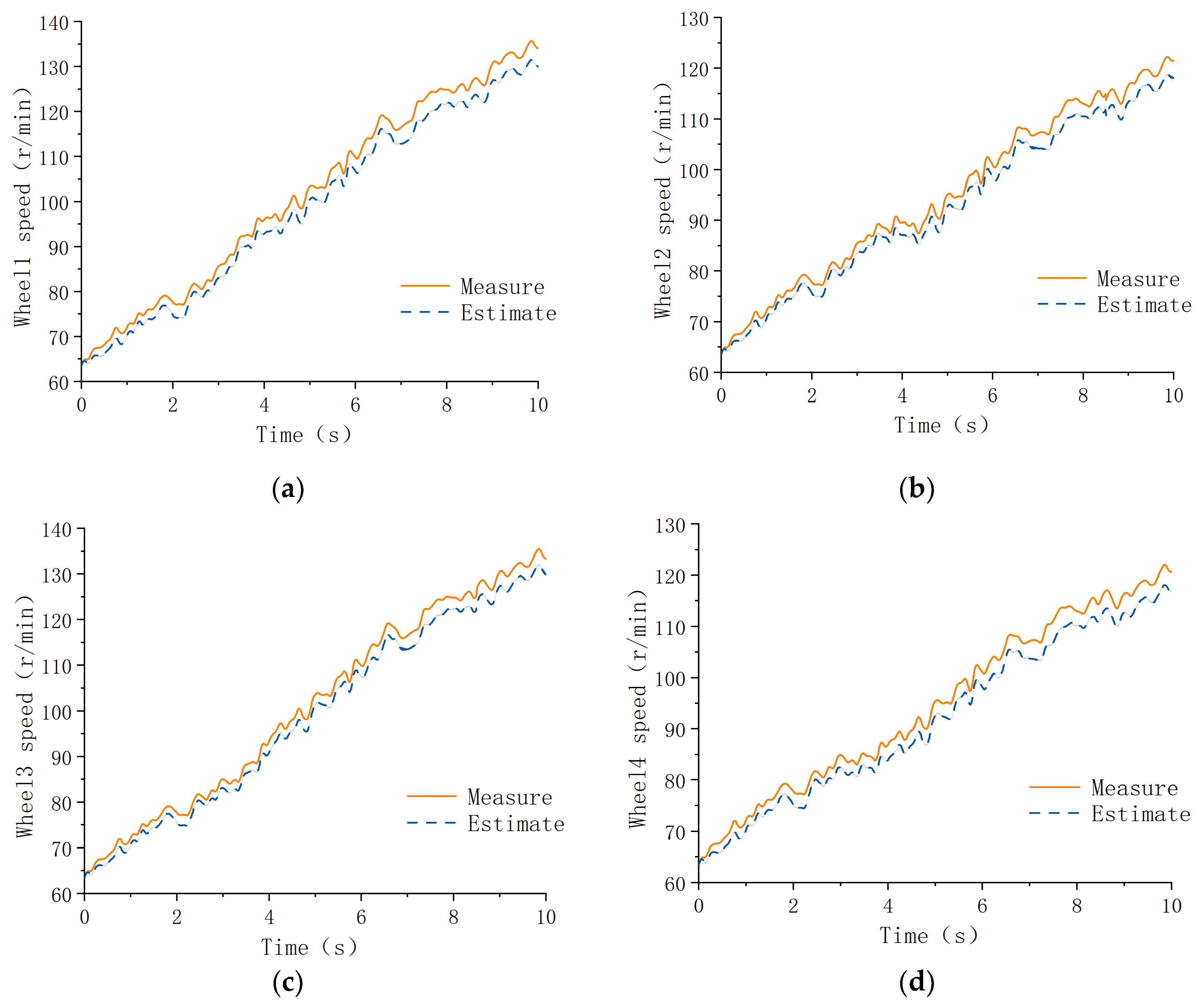
The wheel speed curve is shown in Figure 17. The estimated and measured MAPE values are 1.86%, 1.74%, 1.73%, and 1.63%, respectively. The estimated values are slightly lower than the measured values, and the left wheel’s speed is higher than the right wheel’s speed, which is due to the effect of the pendulum angular velocity during the steering process.

6. Conclusions

In this paper, the state estimation method of key kinetic parameters of distributed electric drive articulated vehicle is investigated. A 7DOF nonlinear dynamics model of a distributed electric drive articulated vehicle is established. Based on the UKF algorithm, a discrete system and observation equations for the articulated vehicle are constructed. To solve the problem that the covariance matrix appears to be non-positive and definite during the estimation process, which leads to a large error or even dispersion, Cholesky decomposition is replaced by SVD decomposition. A forgetting factor is introduced to dynamically adjust the observation noise covariance matrix in real time, which improves the proportion of recent data as well as the convergence and estimation accuracy of the estimation. By improving the UKF algorithm in this way, the estimator is able to adapt to different environments and noises much better, thus improving the estimation. Compared to previous studies, this paper establishes a centralized estimator that contains more estimation parameters, which challenges the convergence and accuracy of the estimation. And it also avoids the mutual influence of the results of estimators at different levels.
The proposed ASVD-UKF parameter state estimation method and UKF estimation method for articulated vehicle dynamics parameter estimation are simulated and compared. The simulation is performed to estimate key dynamic parameters, including the lateral and longitudinal velocities and accelerations, angular velocity, articulated angle, wheel speeds, and longitudinal and lateral tire forces of both the front and rear vehicle bodies. The results demonstrate that the proposed ASVD-UKF method outperforms the UKF estimation method, with smaller errors between the estimated values and reference values, indicating superior estimation performance. Through the principle prototype test, the estimated values of each kinetic parameter are compared and analyzed with the measured values, and the MAPE is less than 7%. The estimation effect is good, so it can meet the strong nonlinear operating characteristics of articulated vehicles, and it validates the articulated vehicle dynamics parameter estimation method.
In this study, vehicle parameters such as the mass, moment of inertia, and center of gravity position are assumed to be known and fixed. However, due to the significant load variations in articulated vehicles, these parameters can change substantially and are difficult to measure directly. In future research, the variation in vehicle body parameters will be considered, and a combined state estimation of both vehicle body parameters and dynamic parameters will be conducted.

Author Contributions

Conceptualization, T.L.; methodology, T.L.; software, T.L. and H.C.; validation, T.L.; formal analysis, T.L.; investigation, T.L. and M.H.; resources, T.L. and M.H.; data curation, T.L. and M.H.; writing—original draft preparation, T.L.; writing—review and editing, T.L. and L.L.; visualization, T.L. and L.L.; supervision, T.L.; project administration, T.L.; funding acquisition, T.L. All authors have read and agreed to the published version of the manuscript.

Funding

This research was funded by the Doctoral Scientific Research Foundation of Hubei University of Automotive Technology, grant number BK202357, and the Hubei Provincial Department of Education Scientific Research Program, grant number Q20231804.

Data Availability Statement

Further inquiries can be directed to the corresponding author.

Acknowledgments

The authors would like to thank all anonymous reviewers and editors for their helpful suggestions for the improvement of this paper.

Conflicts of Interest

The authors declare no conflicts of interest. The funders had no role in the design of the study; in the collection, analyses, or interpretation of data; in the writing of the manuscript; or in the decision to publish the results.

Nomenclature

O 1 x 1 y 1 Front vehicle body coordinate system
O 2 x 2 y 2 Rear vehicle body coordinate system
v x 1 Longitudinal velocity of front vehicle body
v x 2 Longitudinal velocity of rear vehicle body
v y 1 Lateral velocity of front vehicle body
v y 2 Lateral velocity of front vehicle body
ω 1 Angular velocity of z-axis of front vehicle body
ω 2 Angular velocity of z-axis of rear vehicle body
L 1 Distance from center of front vehicle gravity to front axles
L 2 Distance from articulated point to center of front vehicle gravity
L 3 Distance from center of rear vehicle gravity to front axles
L 4 Distance from articulated point to center of rear vehicle gravity
F z j Vertical tire force ( j = 1 , 2 , 3 , 4 )
C σ Longitudinal tire stiffness
C α Lateral tire stiffness
β Swing angle
I 1 Vehicle rotational inertia of z -axis of front vehicle body
I 2 Vehicle rotational inertia of z -axis of rear vehicle body
F x j Longitudinal tire force ( j = 1 , 2 , 3 , 4 )
F y j Lateral tire force ( j = 1 , 2 , 3 , 4 )
M O 1 Torque of steering mechanism on front vehicle body
M O 2 Torque of steering mechanism on rear vehicle body
m 1 Mass of front vehicle body
m 2 Mass of rear vehicle body
F o x 1 Longitudinal force of steering mechanism on front vehicle body
F o x 2 Longitudinal force of steering mechanism on rear vehicle body
F o y 1 Lateral force of steering mechanism on front vehicle body
F o y 2 Lateral force of steering mechanism on rear vehicle body
μ Friction coefficient
R Distance between hinge points of hydraulic cylinder rod and articulated point
r Distance between hinge points of hydraulic cylinder seat and articulated point
θ Initial angle of hydraulic cylinder
StiTire slip rate ( i = 1 , 2 , 3 , 4 )
α Tire slip angle
T t i Wheel drive torque ( i = 1 , 2 , 3 , 4 )

Appendix A

Related Calculation for Vehicle Dynamics Model

Equilibrium equations for the longitudinal, lateral, and yaw of the articulated vehicle’s front and rear bodies:
m 1 v ˙ x 1 v y 1 ω 1 = F x 1 + F x 2 + F o x 1 m 1 v ˙ y 1 + v x 1 ω 1 = F y 1 + F y 2 F o y 1 I 1 w ˙ 1 = M O 1 + ( F x 1 F x 2 ) B + ( F y 1 + F y 2 ) L 1 + F o y 1 L 2
m 2 v ˙ x 2 v y 2 ω 2 = F x 3 + F x 4 F o x 2 cos β F o y 2 sin β m 2 v ˙ y 2 + v x 2 ω 2 = F y 3 + F y 4 F o x 2 sin β + F o y 2 cos β I 2 ω ˙ 2 = M O 2 + ( F x 3 F x 4 ) B ( F y 3 + F y 4 ) L 3 + F o y 2 cos β F o x 2 sin β L 4
The kinematic relationships between the front and rear vehicle bodies are as follows:
v x 2 = v x 1 cos β v y 1 L 2 ω 1 sin β v y 2 = v x 1 sin β + v y 1 L 2 ω 1 cos β L 4 ω 2
v ˙ x 2 = v ˙ x 1 cos β v ˙ y 1 L 2 ω ˙ 1 sin β v y 1 cos β + v x 1 sin β L 2 ω 1 cos β ω 1 ω 2 v ˙ y 2 = v ˙ x 1 sin β + v ˙ y 1 L 2 ω ˙ 1 cos β L 4 ω ˙ 2 + v x 1 cos β v y 1 sin β + L 2 ω 1 sin β ω 1 ω 2
β ˙ = ω 1 ω 2
The parameters related to the calculation of the articulated vertical force distribution are as follows:
a x = m 1 a x 1 cos θ 1 m 1 a y 1 sin θ 1 + m 2 a x 2 cos θ 2 + m 2 a y 2 sin θ 2 m 1 + m 2 a y = m 1 a x 1 sin θ 1 + m 1 a y 1 cos θ 1 m 2 a x 2 sin θ 2 + m 2 a y 2 cos θ 2 m 1 + m 2
L = L 1 + L 2 2 + L 3 + L 4 2 2 L 1 + L 2 L 3 + L 4 cos ( π β ) L m = L 2 2 + L 4 2 2 L 2 L 4 cos ( π β ) L m f = m 2 m 1 + m 2 L m L m r = m 1 m 1 + m 2 L m
θ 2 = arccos L 3 + L 4 2 + L 2 L 1 + L 2 2 2 L 3 + L 4 L θ 1 = β θ 2 Δ B = L 3 sin θ 2
L l f = L m f + L 1 cos θ 1 + B sin θ 1 L l r = L m r + L 3 cos θ 2 + B sin θ 2 L r f = L m f + L 1 cos θ 1 B sin θ 1 L r r = L m r + L 3 cos θ 2 B sin θ 2

Appendix B

Tire force calculation-related parameters.
Longitudinal line speed of each wheel center:
v t x 1 = v x 1 + B w 1 v t x 2 = v x 1 B w 1 v t x 3 = v x 2 + B w 2 v t x 4 = v x 2 B w 2
Lateral line speed of each wheel center:
v t y 1,2 = v y 1 + L 1 w 1 v t y 3,4 = v y 2 L 3 w 2
Angular acceleration, tire slip angle, and tire slip rate of each wheel:
ω ˙ t i = T t i F x i + F z i f r I t i
α t i = arctan v t y i v t x i
S t i = v t x i r ω t i r ω t i

Appendix C

For the lateral and longitudinal accelerations of the front and rear bodies, the longitudinal and lateral tire forces, the f i = 0 , and the remaining parameters are
f 1 = w 1 ( k ) v y 1 ( k ) + m 2 L 4 w ˙ 2 ( k ) sin β ( k ) m 2 L 2 w 1 2 ( k ) m 2 L 4 w 2 2 ( k ) cos β ( k ) + F x 1 ( k ) + F x 2 ( k ) + F x 3 ( k ) + F x 4 ( k ) cos β ( k ) + F y 3 ( k ) + F y 4 ( k ) sin β ( k ) / m 1 + m 2
f 2 = w 1 ( k ) v x 1 ( k ) + m 2 L 2 w ˙ 1 ( k ) + m 2 L 4 w ˙ 2 ( k ) cos β ( k ) + m 2 L 4 w 2 2 ( k ) sin β ( k ) + F y 1 ( k ) + F y 2 ( k ) + F y 3 ( k ) + F y 4 ( k ) cos β ( k ) F x 3 ( k ) + F x 4 ( k ) sin β ( k ) / m 1 + m 2
x 3 ( k + 1 ) = m 2 L 4 w ˙ 2 ( k ) sin β ( k ) m 2 L 2 w 1 2 ( k ) m 2 L 4 w 2 2 ( k ) cos β ( k ) + F x 1 ( k ) + F x 2 ( k ) + F x 3 ( k ) + F x 4 ( k ) cos β ( k ) + F y 3 ( k ) + F y 4 ( k ) sin β ( k ) / m 1 + m 2
x 4 ( k + 1 ) = m 2 L 2 w ˙ 1 ( k ) + m 2 L 4 w ˙ 2 ( k ) cos β ( k ) + m 2 L 4 w 2 2 ( k ) sin β ( k ) + F y 1 ( k ) + F y 2 ( k ) + F y 3 ( k ) + F y 4 ( k ) cos β ( k ) F x 3 ( k ) + F x 4 ( k ) sin β ( k ) / m 1 + m 2
f 5 = M O ( k ) + F x 1 ( k ) F x 2 ( k ) B + F y 1 ( k ) + F y 2 ( k ) L 1 + L 2 m 1 v ˙ y 1 ( k ) + v x 1 ( k ) ω 1 ( k ) L 2 / I 1
f 6 = v ˙ x 1 ( k ) cos β ( k ) v ˙ y 1 ( k ) L 2 ω ˙ 1 ( k ) sin β ( k ) v y 1 ( k ) cos β ( k ) + v x 1 ( k ) sin β ( k ) L 2 ω 1 ( k ) cos β ( k ) ω 1 ( k ) ω 2 ( k )
f 7 = v ˙ x 1 ( k ) sin β ( k ) + v ˙ y 1 ( k ) L 2 ω ˙ 1 ( k ) cos β ( k ) L 4 ω ˙ 2 ( k ) + v x 1 ( k ) cos β ( k ) v y 1 ( k ) sin β ( k ) + L 2 ω 1 ( k ) sin β ( k ) ω 1 ( k ) ω 2 ( k )
f 8 = v ˙ x 1 ( k ) cos β ( k ) v ˙ y 1 ( k ) L 2 ω ˙ 1 ( k ) sin β ( k ) v y 1 ( k ) cos β ( k ) + v x 1 ( k ) sin β ( k ) L 2 ω 1 ( k ) cos β ( k ) ω 1 ( k ) ω 2 ( k ) w 2 ( k ) v y 2 ( k )
f 9 = v ˙ x 1 ( k ) sin β ( k ) + v ˙ y 1 ( k ) L 2 ω ˙ 1 ( k ) cos β ( k ) L 4 ω ˙ 2 ( k ) + v x 1 ( k ) cos β ( k ) v y 1 ( k ) sin β ( k ) + L 2 ω 1 ( k ) sin β ( k ) ω 1 ( k ) ω 2 ( k ) + w 2 ( k ) v x 2 ( k )
f 10 = M O ( k ) + F x 3 ( k ) F x 4 ( k ) B + F y 1 ( k ) + F y 2 ( k ) L 4 cos β ( k ) F x 1 ( k ) + F x 2 ( k ) L 4 sin β ( k ) F y 3 ( k ) + F y 4 ( k ) L 3 m 1 v ˙ y 1 ( k ) + v x 1 ( k ) ω 1 ( k ) L 4 cos β ( k ) m 1 v ˙ x 1 ( k ) v y 1 ( k ) ω 1 ( k )
f 11 = ω 1 ( k ) ω 2 k   f 12 = T t 1 F x 1 ( k ) + F z 1 ( k ) f r / I r     f 13 = T t 2 F x 2 ( k ) + F z 2 ( k ) f r / I r f 14 = T t 3 F x 3 ( k ) + F z 3 ( k ) f r / I r       f 15 = T t 4 F x 4 ( k ) + F z 4 ( k ) f r / I r

References

  1. Gao, L.; Dong, Y.; Zhao, J. Dynamic Modeling and Characteristic Analysis of Articulated Steering Vehicles. Appl. Sci. 2023, 13, 5099. [Google Scholar] [CrossRef]
  2. Azad, N.L.; Khajepour, A.; Mcphee, J. A survey of stability enhancement strategies for articulated steer vehicles. Int. J. Heavy Veh. Syst. 2009, 16, 26. [Google Scholar] [CrossRef]
  3. Guo, H.; Cao, D.; Chen, H.; Lv, C.; Wang, H.; Yang, S. Vehicle Dynamic State Estimation: State of the Art Schemes and Perspectives. IEEE-CAA J. Autom. Sin. 2018, 5, 418–431. [Google Scholar] [CrossRef]
  4. Hong, S.; Lee, C.; Borrelli, F.; Hedrick, J.K. A Novel Approach for Vehicle Inertial Parameter Identification Using a Dual Kalman Filter. IEEE Trans. Intell. Transp. Syst. 2015, 16, 151–161. [Google Scholar] [CrossRef]
  5. Mosconi, L.; Farroni, F.; Sakhnevych, A.; Timpone, F.; Gerbino, F.S. Adaptive vehicle dynamics state estimator for onboard automotive applications and performance analysis. Veh. Syst. Dyn. 2023, 61, 3244–3268. [Google Scholar] [CrossRef]
  6. Wang, C.; Wang, Z.; Zhang, L.; Cao, D.; Dorrell, D.G. A Vehicle Rollover Evaluation System Based on Enabling State and Parameter Estimation. IEEE Trans. Ind. Inform. 2021, 17, 4003–4013. [Google Scholar] [CrossRef]
  7. Rezaei, O.; Moghaddam, H.A.; Papari, B. A fast sliding-mode-based estimation of state-of-charge for Lithium-ion batteries for electric vehicle applications. J. Energy Storage 2022, 45, 103484. [Google Scholar] [CrossRef]
  8. Yang, C.; Zhu, Q.; Liu, Q.; Chen, X. An unscented Kalman filter based velocity estimation method for articulated steering vehicle using a novel dynamic model. Proc. Inst. Mech. Eng. Part K J. Multi-Body Dyn. 2023, 237, 389–405. [Google Scholar] [CrossRef]
  9. Tan, C.; Cai, Y.; Wang, H.; Sun, X.; Chen, L. Vehicle State Estimation Combining Physics-Informed Neural Network and Unscented Kalman Filtering on Manifolds. Sensors 2023, 23, 6665. [Google Scholar] [CrossRef] [PubMed]
  10. Xing, Y.; Lv, C. Dynamic State Estimation for the Advanced Brake System of Electric Vehicles by Using Deep Recurrent Neural Networks. IEEE Trans. Ind. Electron. 2020, 67, 9536–9547. [Google Scholar] [CrossRef]
  11. Heidfeld, H.; Schünemann, M.; Kasper, R. UKF-based State and tire slip estimation for a 4WD electric vehicle. Veh. Syst. Dyn. 2020, 58, 1479–1496. [Google Scholar] [CrossRef]
  12. Hashemi, E.; Khosravani, S.; Khajepour, A.; Kasaiezadeh, A.; Chen, S.-K.; Litkouhi, B. Longitudinal vehicle state estimation using nonlinear and parameter-varying observers. Mechatronics 2017, 43, 28–39. [Google Scholar] [CrossRef]
  13. Jin, X.; Yin, G.; Chen, N. Advanced Estimation Techniques for Vehicle System Dynamic State: A Survey. Sensors 2019, 19, 4289. [Google Scholar] [CrossRef] [PubMed]
  14. Ahmadi Jeyed, H.; Ghaffari, A. Nonlinear estimator design based on extended Kalman filter approach for state estimation of articulated heavy vehicle. Proc. Inst. Mech. Eng. Part K J. Multi-Body Dyn. 2019, 233, 254–265. [Google Scholar] [CrossRef]
  15. Ziaukas, Z.; Wielitzka, M.; Ortmaier, T.; Kobler, J.-P. Simultaneous Estimation of Steering and Articulation Angle in a Truck-Semitrailer Combination Solely Based on Trailer Signals. In Proceedings of the 2019 American Control Conference (ACC), Philadelphia, PA, USA, 10–12 July 2019; IEEE: Piscataway, NJ, USA, 2019; pp. 2509–2514. [Google Scholar] [CrossRef]
  16. Ehlers, S.F.G.; Sourkounis, P.; Ziaukas, Z.; Kobler, J.-P.; Jacob, H.-G. Optimized Tuning of an EKF for State and Parameter Estimation in a Semitrailer. In Proceedings of the International Symposium on Advanced Vehicle Control, Kanagawa, Japan, 12–16 September 2022; Kanagawa Institute of Technology: Atsugi, Japan, 2024. [Google Scholar]
  17. Wenwei, W.; Yifan, Z.; Wei, Z.; Cheng, L. Yaw Stability Control Strategy of Multi-wheel Independent Electric Articulated Bus. J. Mech. Eng. 2020, 56, 161. [Google Scholar] [CrossRef]
  18. Gao, L.; Ma, F.; Jin, C. A Model-Based Method for Estimating the Attitude of Underground Articulated Vehicles. Sensors 2019, 19, 5245. [Google Scholar] [CrossRef] [PubMed]
  19. Lin, C.; Cheng, X.; Zhang, H.; Gong, X. Estimation of Center of Gravity Position for Distributed Driving Electric Vehicles Based on Combined H∞-EKF Method. Energy Procedia 2016, 88, 970–977. [Google Scholar] [CrossRef]
  20. Yang, Z.; Wang, J.; Han, Y. A Novel Real-Time Center of Gravity Estimation Method for Wheel Loaders with Front/Rear-Axle-Independent Electric Driving. J. Control Sci. Eng. 2021, 2021, 6621060. [Google Scholar] [CrossRef]
  21. Gao, G.; Wang, J.; Ma, T.; Liu, W.; Lei, T. Multistage Estimators for the Distributed Drive Articulated Steering Vehicle. Math. Probl. Eng. 2020, 2020, 5921285. [Google Scholar] [CrossRef]
  22. Lei, T.; Gu, X.; Zhang, K.; Li, X.; Wang, J. PSO-Based Variable Parameter Linear Quadratic Regulator for Articulated Vehicles Snaking Oscillation Yaw Motion Control. Actuators 2022, 11, 337. [Google Scholar] [CrossRef]
  23. Dugoff, H.; Fancher, P.S.; Segel, L. Tire Performance Characteristics Affecting Vehicle Response to Steering and Braking Control Inputs; National Academy of Sciences: Washington, DC, USA, 1969. [Google Scholar]
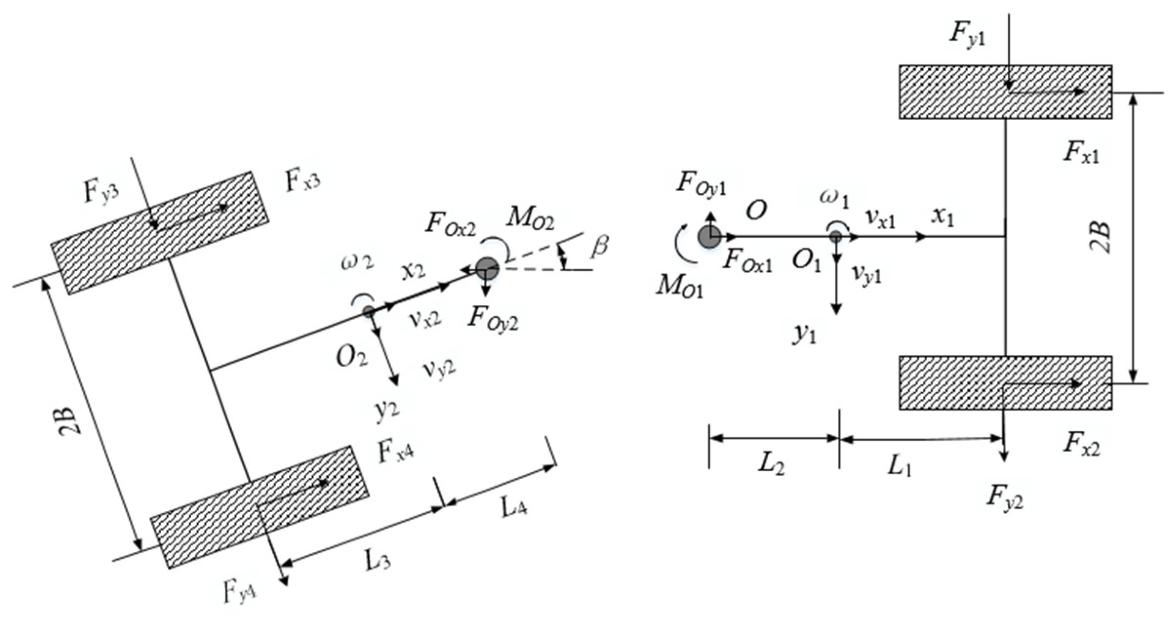
Figure 1. Articulated vehicle dynamics model.
Actuators 14 00031 g001
Figure 2. Articulated vehicle vertical load analysis.
Actuators 14 00031 g002
Figure 3. The SVD-UKF estimation flowchart.
Actuators 14 00031 g003
Figure 4. Target velocity and articulated angle. (a) Longitudinal and velocity of front of vehicle; (b) articulated angle.
Actuators 14 00031 g004
Figure 5. Simulation system flow chart.
Actuators 14 00031 g005
Figure 6. Longitudinal and lateral velocity estimation results. (a) Longitudinal velocity of front vehicle body, (b) longitudinal velocity of rear vehicle body, (c) lateral velocity of front vehicle body, and (d) lateral velocity of rear vehicle body.
Actuators 14 00031 g006
Figure 7. Longitudinal and lateral acceleration estimation results. (a) Longitudinal acceleration of front vehicle body, (b) longitudinal acceleration of rear vehicle body, (c) lateral acceleration of front vehicle body, and (d) lateral acceleration of rear vehicle body.
Actuators 14 00031 g007
Figure 8. Angular velocity and articulated angle estimation results. (a) Angular velocity of front vehicle body, (b) angular velocity of rear vehicle body, and (c) articulated angle.
Actuators 14 00031 g008
Figure 9. Wheel speed estimation results: (a) tire 1 speed, (b) tire 2 speed, (c) tire 3 speed, and (d) tire 4 speed.
Actuators 14 00031 g009aActuators 14 00031 g009b
Figure 10. Tire longitudinal force estimation results: (a) tire 1 longitudinal force, (b) tire 2 longitudinal force, (c) tire 3 longitudinal force, and (d) tire 4 longitudinal force.
Actuators 14 00031 g010
Figure 11. Tire lateral force estimation results: (a) tire 1 lateral force, (b) tire 2 lateral force, (c) tire 3 lateral force, and (d) tire 4 lateral force.
Actuators 14 00031 g011
Figure 12. Distributed electric drive principle prototype vehicle (1—vehicle frame; 2—control system; 3—steering system; 4—drive system).
Actuators 14 00031 g012
Figure 13. Flowchart of state estimation method validation.
Actuators 14 00031 g013
Figure 14. Longitudinal and lateral velocity estimation results. (a) Longitudinal velocity of front vehicle body; (b) lateral velocity of front vehicle body.
Actuators 14 00031 g014
Figure 15. Angular velocity and articulated angle estimation results. (a) Angular velocity of front vehicle body, (b) angular velocity of rear vehicle body, and (c) articulated angle.
Actuators 14 00031 g015
Figure 16. Longitudinal and lateral acceleration estimation results. (a) Longitudinal acceleration of front vehicle body, (b) longitudinal acceleration of rear vehicle body, (c) lateral acceleration of front vehicle body, (d) lateral acceleration of rear vehicle body.
Actuators 14 00031 g016
Figure 17. Wheel speed estimation results: (a) wheel 1 speed, (b) wheel 2 speed, (c) wheel 3 speed, and (d) wheel 4 speed.
Actuators 14 00031 g017
Table 1. Sensor information.
NameQuantityLocationMeasured Parameters
IMU2front and rear bodies a x 1   a y 1   ω 1   a x 2   a y 2   ω 2   (Equation (26))
drive torque44 hub motors T t 1   T t 2   T t 3   T t 4 (Equation (29))
steering torque1steering system M O  (Equation (29))
wheel speed44 hub motors ω t 1   ω t 2   ω t 3   ω t 4  (Equation (26))
articulated
angle
1steering system β
RTK1front body v x 1   v y 1  (Equation (24))
Disclaimer/Publisher’s Note: The statements, opinions and data contained in all publications are solely those of the individual author(s) and contributor(s) and not of MDPI and/or the editor(s). MDPI and/or the editor(s) disclaim responsibility for any injury to people or property resulting from any ideas, methods, instructions or products referred to in the content.