Optimization Design of Permanent Magnet Synchronous Motor Based on Multi-Objective Artificial Hummingbird Algorithm

Abstract

The interior permanent magnet synchronous motor (IPMSM) is known for its high output torque, strong overload capacity, and high power density, making it a popular choice in the electric vehicle industry. This paper proposes an improved multi-objective artificial hummingbird algorithm that combines chaotic mapping, adaptive weights, and dynamic crowding entropy. An optimization strategy that combines the Taguchi method with the Improved Multi-Objective Artificial Hummingbird Algorithm (IMOAHA), is proposed to minimize torque ripple and back electromotive force in the interior permanent magnet synchronous motor while simultaneously increasing the average torque of the motor. Taking the 8-pole 48-slot interior permanent magnet synchronous motor as an example, the optimization objectives include back electromotive force, average torque, and torque ripple. The rotor-related structural parameters are used as optimization variables. First, the Taguchi method is employed to identify parameters that significantly influence the optimization objectives. Subsequently, response surface fitting is used to establish the relationship between the optimization objectives and parameters. Finally, the multi-objective artificial hummingbird algorithm is utilized for optimization. By comparing the finite element analysis of the motor models before and after optimization, it is evident that the improved multi-objective artificial hummingbird algorithm can effectively enhance the performance of the interior permanent magnet synchronous motor.

1. Introduction

With the rapid development of modern industry, permanent magnet synchronous motors (PMSMs) are extensively utilized in various fields such as power, transportation, aerospace, etc. They are favored for their compact size, high torque output, and exceptional efficiency [1,2]. However, as the demand for energy efficiency, environmental sustainability, and safety continues to rise, there is an increasing need for improved performance and stability of PMSMs. Consequently, optimizing PMSMs becomes particularly crucial to meeting these evolving requirements.

The conventional design approach for PMSM typically emphasizes a single objective, focusing solely on individual motor performance aspects such as maximizing torque or minimizing losses, which leads to poor overall motor performance. Reference [3] enhanced the electromagnetic vibration force of the stator teeth by adding the auxiliary slot structure of the motor rotor and conducted a comparative analysis of the results before and after optimization. This optimization has been proven to effectively decrease the noise and vibration of the motor while ensuring its electromagnetic performance. Reference [4] employed the Taguchi method for structural design to mitigate the peak air gap flux density of the external rotor PMSMs resulting from slotting the stator. Reference [5] introduced a magnetic barrier structure on the motor rotor to address the issue of uneven saturation of the rotor-side magnetic bridge. Additionally, the study utilized the Taguchi method to optimize the structural parameters of the added magnetic barrier. Subsequently, it analyzed the influence of these parameters on the electromagnetic performance of the motor. The findings suggest that maximizing the output torque is desirable without altering the no-load back electromotive force (EMF) and torque ripple. Reference [6] introduces a new torque ripple model, which utilizes a genetic algorithm to optimize the amplitude and phase angle of stator harmonic current, effectively reducing torque ripple.

Single objective optimization is straightforward, intuitive, and easy to implement. However, in motor optimization design, multi-objective optimization is often encountered, with these objectives frequently imposing constraints on each other. Hence, in the optimization design process of PMSM, it becomes imperative to strike a balance among multiple objective functions, including motor efficiency, torque density, volume, and weight. To address the mutual constraints between these multiple objectives, researchers have increasingly turned to multi-objective optimization algorithms, enabling a more comprehensive and balanced design of PMSM.

Currently, commonly used multi-objective optimization algorithms include multi-objective particle swarm optimization (MOPSO) [7], non-dominated sorting genetic algorithm (NSGA-II) [8], multi-objective grey wolf algorithm (MOGWO) [9], multi-objective evolutionary algorithm (MODA) [10], multi-objective cuckoo algorithm (MOCS) [11], and multi-objective artificial hummingbird algorithm (MOAHA) [12]. The MOPSO algorithm is grounded in the concept of swarm intelligence. It offers the advantages of robust global search capability and rapid convergence speed. However, it is susceptible to getting trapped in local optima when handling high-dimensional problems. NSGA-II is rooted in the principles of natural evolution. It demonstrates strong convergence and search efficiency, but it may have limitations in handling high-dimensional problems. MOGWO draws inspiration from the predatory behavior of gray wolves. It possesses good convergence and diversity, but its capability to solve complex problems may be limited. MODA adopts the concept of evolution and is effective in exploring the solution space, but its performance may be limited in high-dimensional problems. MOCS simulates the foraging behavior of bird flocks. It exhibits strong global search ability but may encounter challenges when dealing with high-dimensional problems. MOAHA simulates the foraging behavior of hummingbirds, leveraging the benefits of diversity and efficiency. It can maintain population diversity and quickly identify the optimal solution set. However, when addressing complex problems, the algorithm’s convergence may be limited, and it may be prone to getting trapped in local optima. Reference [12] has demonstrated, through a series of comprehensive experimental verifications, that the multi-objective artificial hummingbird algorithm exhibits superior performance in terms of convergence accuracy, diversity of solution sets, and spatial distribution when solving 28 typical benchmark problems. It surpasses several other multi-objective optimization algorithms, including multi-objective particle swarm optimization, non-dominated inheritance algorithm, decomposition evolution strategy, strength evolution algorithm, multi-objective ant optimization, multi-objective salt swarm algorithm, multi-objective wolf swarm algorithm, and multi-objective grey wolf algorithm. In essence, this study strongly validates the efficiency and leading advantages of the multi-objective artificial hummingbird algorithm in the realm of multi-objective optimization. Therefore, this paper uses a multi-objective artificial hummingbird algorithm as the optimization algorithm.

Reference [13] proposes a multi-objective hierarchical optimization method based on parameter hierarchical design, combined with the Taguchi method and response surface method (RSM). This method is applied to optimize the rotor surface slot parameters of a V-type interior permanent magnet synchronous motor (IPMSM). By comparing the electromagnetic performance of the motor before and after optimization, it can be concluded that the optimized motor not only improves the output torque but also reduces the torque ripple. Reference [14] proposes a multi-objective optimization method for improving the torque performance of IPMSM using a single-layer fractional slot concentrated winding. By performing parameter design on the rotor slots and employing the RSM and the seagull optimization algorithm to obtain the optimal parameter design and determine the optimal slot position. The results indicate that the optimized design leads to a reduction in torque ripple and an increase in average torque. Reference [15] presents a multi-objective optimization design method for PMSM based on the artificial bee colony algorithm, with efficiency and the electromechanical time constant set as the optimization objectives. Through finite element analysis, the optimized motor exhibits improved efficiency and reduced mechanical time constant. Reference [16] presents a novel comprehensive multi-objective optimization design method for a spoke-type permanent magnet motor, utilizing sensitivity analysis, RSM, and the basic multi-objective particle swarm algorithm to conduct robustness analysis of the motor. The results indicate that this optimization method not only reduces torque ripple but also enhances the reliability and robustness of the machine. Reference [17] designed a new type of automotive permanent magnet synchronous motor (IPMSM) and conducted multi-objective optimization using the Taguchi method to reduce torque ripple and cogging torque. Reference [18] utilized the Quantum Bat Algorithm (QBA) and Pyramid Neural Network (PNN) model to optimize the structural parameters of a High-Speed Permanent Magnet Synchronous Motor (HPMSM) and determine the optimal combination to minimize motor losses. The performance of the optimized HPMSM was validated through finite element simulation analysis and prototype experiments. Reference [19] developed an optimal model for the PMSM prototype of an electric compressor and verified the efficiency of optimizing PMSM using the optimal Latin hypercube, Kriging model, and genetic algorithm. However, [13,14,15,16,17,18,19] transforms multi-objective optimization into single-objective optimization by determining the trade-off relationship between multiple objectives, and the allocation of weights usually requires subjective judgment. Therefore, this process may not be objective enough and may lead to results biased towards a specific objective at the expense of other objectives.

Reference [20] presents a multi-objective optimization design based on the rotor topology of a permanent magnet-assisted bearingless synchronous reluctance motor. The study combines sensitivity analysis with NSGA-II to select the optimal design variables. The research results demonstrate that the optimized motor exhibits higher average torque, average suspension force, and power factor. However, this method requires setting target function values in advance and may not effectively illustrate the relationships among multiple objectives. Reference [21] introduces a multi-objective optimal rotor design method for an IPMSM based on finite element analysis (FEA). Sensitivity analysis is used to determine the appropriate range and initial values of each parameter, and the average torque and torque ripple of the IPMSM are optimized. Reference [22] introduces a convolutional neural network model based on deep learning, which achieves rotor topology optimization for IPMSM. The results indicate that this method improves computational speed and average torque without compromising search capability. However, this method only considers average torque and does not take into account other performance aspects of the motor. Reference [23] presents a multi-objective design optimization method for PMSLM based on machine learning algorithms. By optimizing the motor’s structural parameters, it achieves the optimal performance of high average thrust, low thrust ripple, and low total harmonic distortion. However, deep learning requires a large amount of data for training, as well as larger model scales and parameter quantities, which can make model deployment and maintenance more complex.

In summary, the utilization of multi-objective optimization algorithms has become a highly effective method for achieving optimal and balanced performance in the design of PMSM. These algorithms enable designers to consider multiple objectives simultaneously and find comprehensive solutions that can meet different application requirements. While multi-objective optimization algorithms have great potential in PMSM design, there is still some subjectivity and difficulties in balancing the relationships between various objectives and selecting the best solution.

To address the issue of traditional MOAHA algorithms easily falling into local optima too early, this paper introduces chaotic mapping Bernoulli to initialize the population, nonlinear increasing adaptive weights, and an external file maintenance mechanism based on dynamic crowding entropy to improve the multi-objective artificial hummingbird optimization algorithm (IMOAHA). To effectively overcome the problem of getting stuck in local optima, this paper integrates the Taguchi method and the IMOAHA algorithm to conduct multi-objective optimization design on IPMSM, while considering average torque, torque ripple, iron loss, and EMF. The accuracy of the multi-objective optimization design is validated through finite element simulation.

The rest of this paper is structured as follows. Section 2 provides a brief introduction and enhancement of the MOAHA. The optimization methods are presented in Section 3. Section 4 details the finite element simulation results. Finally, the findings of this paper are summarized in Section 5.

2. IPMSM Basic Structure

Surface-mounted permanent magnet synchronous motors (SPMSMs) and IPMSMs are two types of PMSMs, distinguished by the placement positions of the permanent magnets. While SPMSMs exhibit low torque ripple, they have lower power density. Furthermore, at high speeds, SPMSMs are susceptible to permanent magnet detachment. The IPMSMs offer high output torque, a wide speed range, and high efficiency, making them suitable for various industrial production and other fields.

The rotor structures of the interior permanent magnet synchronous motor include “1-shaped”, “V-shaped”, and “V + 1-shaped”, each differing in structure and performance. The “1-shaped” rotor has a simple structure but low magnetic flux density, making it unsuitable for high-speed applications. The “V-shaped” rotor structure offers high magnetic flux density and is suitable for high-speed applications. However, the difference in magnetic circuit impedance between the d-axis and q-axis is small, resulting in lower reluctance torque. The “V + 1-shaped” structure is a hybrid of the “1-shaped” and “V-shaped” designs, featuring a short magnetic circuit, low magnetic resistance, higher magnetic properties, and stronger magnetic field strength [24]. Therefore, this paper utilizes the “V + 1-shaped” IPMSM. Compared to full-pitch windings, shorted-pitch windings offer several advantages in motor design. These include reducing harmonics, enhancing the electromotive force waveform, improving efficiency and power factor, minimizing torque fluctuations, boosting dynamic response and stability, and lowering iron losses. These benefits collectively contribute to an overall enhancement of motor performance.

The electromagnetic torque formula for permanent magnet synchronous motors is [25]:

$$T_e=\frac{3}{2}p\left[{\psi }_f{i}_q+\left(L_d-L_q\right)i_d{i}_q\right]$$

(1)

where p is the number of pole pairs, ψ_f is the permanent magnet flux linkage, i_d, and i_q are the d-axis and q-axis current, respectively, and L_d and L_q are the d-axis and q-axis inductance, respectively.

The average torque magnitude (T_avg) of the interior permanent magnet synchronous motor can be defined as the peak-to-peak average of the electromagnetic torque (T_e) during steady operation of the motor as follows:

$$T_{avg}=avg(T_e)$$

(2)

The torque ripple T_ripple used in this paper can be defined as the peak-to-peak difference of electromagnetic torque, as shown below:

$$T_{ripple}=T_{\max }-T_{\min }$$

(3)

where avg means the calculated average, T_max is the maximum peak of the electromagnetic torque and T_min is the minimum peak of the electromagnetic torque.

The permanent magnet synchronous motor adopts a separate calculation model that divides iron loss into three parts [26]:

$$P_{fe}=P_h+P_c+P_e$$

(4)

$$P_h=k_{h}f{B}_p^x$$

(5)

$$P_c=k_c{f}^2{B}_p^2$$

(6)

$$P_e=k_e{f}^{1.5}{B}_P^{1.5}$$

(7)

where, P_h, P_c, and P_e represent hysteresis loss, classical eddy current loss, and anomalous eddy current loss, respectively. B_p represents magnetic flux density amplitude, f represents frequency, k_h, x represents hysteresis loss coefficient, k_c represents classical eddy current loss coefficient, and k_e represents anomalous loss coefficient.

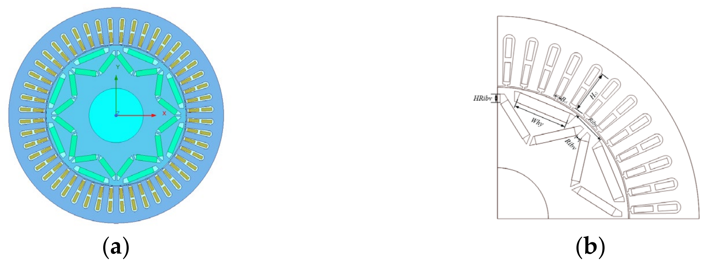
This paper focuses on the finite element model of a three-phase 8-pole 48-slot IPMSM, as depicted in Figure 1. The motor stator features a double-layer shorted pitch, while the rotor structure utilizes a “V + 1-shaped” design. The number of slots for the shorted pitch winding is five. The primary parameters of the IPMSM finite element model are presented in

Table 1. Interior permanent magnet synchronous motor parameters.

Parameter	Value	Parameter	Value
Rated power/kW	15	Slot body height Hs2/mm	25.6
Outer diameter of stator/mm	238	Slot wedge maximum width Bs1/mm	3.6
Inter diameter of stator/mm	156	Rib width of 1-shaped PM Riby/mm	21
Outer diameter of rotor/mm	154.6	Width of 1-shaped PM Why/mm	30
Thickness of permanent magnet/mm	6	Rib width of V-shaped PM Ribv/mm	1
Air gap length/mm	0.7	Rib height of V-shaped PM HRibv/mm	5
Number of poles	8	Distance from V-shaped permanent magnet to shaft O2v/mm	18
Number of slots	48	Side distance of V-shaped permanent magnet DMv/mm	2
Core length/mm	60	Rated speed/rpm	3000
d-axis inductance/mH	6.43	d-axis flux linkage/Wb	0.26
q-axis inductance/mH	14.66	q-axis flux linkage/Wb	−0.18
Number of conductors per slot	10	Conductor dimensions/mm	1.085

.

The model of the internal permanent magnet synchronous motor was constructed according to Table 1, and materials were assigned to each component as presented in

Table 2. Main structural materials for internal permanent magnet synchronous motors.

Motor Components	Material	Motor Components	Material
Stator core	DW310_35	Coil	Copper_75C
Rotor core	DW310_35	Permanent magnet	NdFe35
Rotor motion area	Vacuum

.

3. Improved Multi-Objective Artificial Hummingbird Algorithm

3.1. Multi-Objective Artificial Hummingbird Algorithm

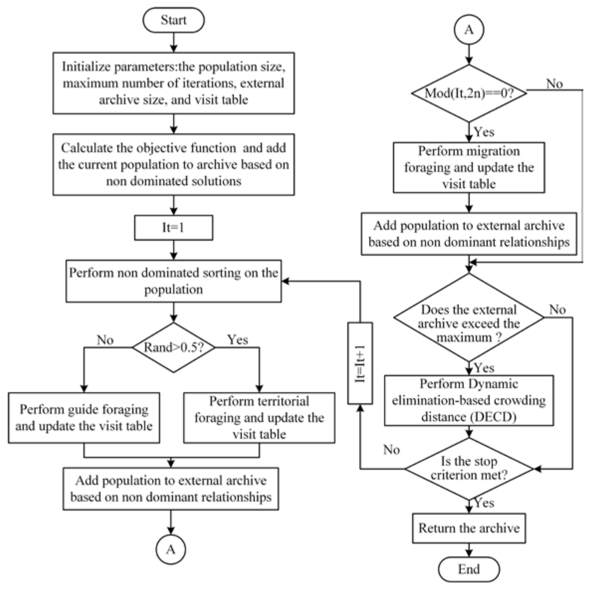
The multi-objective artificial hummingbird algorithm simulates the unique flight capabilities and intelligent foraging strategies observed in hummingbirds in nature [12]. It establishes three flight skill models for foraging strategies, encompassing axial flight, diagonal flight, and omnidirectional flight. Moreover, it achieves guided foraging, territorial foraging, and migratory foraging. An access table is constructed to simulate the memory function of hummingbirds regarding food sources. The MOAHA algorithm flowchart is depicted in Figure 2.

• Population Initialization

A population of n hummingbirds is placed on n food sources randomly initialized as follows [12]:

$$x_i=Low+r\ast \left(Up-Low\right)\hspace{1em}\hspace{1em}i=1,\dots ,n$$

(8)

where Low and Up are the upper and lower boundaries of the d-dimensional problem, r is a random number in the range of [0, 1], and x_i represents the position of the i-th food source.

The initialization of the access table for food sources is as follows:

$$V{T}_{i,j}=\left\{\begin{array}{l} 0\hspace{1em}if i\ne j\\ null\hspace{1em}i=j\end{array}\right.\hspace{1em}\hspace{1em}i=1,\dots ,n;j=1,\dots ,n$$

(9)

where i = j, VT_i,j = null indicates that hummingbirds feed on specific food sources; i ≠ j, VT_i,j = 0 indicates that the j-th hummingbird has just visited the i-th food source in the current iteration.

2.

Guide Foraging

During the foraging process, each hummingbird initially identifies the food source with the highest level of access and then selects the food source with the highest nectar supplementation rate from these sources as the target food source. Hummingbirds utilize directional switching vectors to control the direction of flight, assisting them in exploring the environment more effectively and finding the optimal food source.

These flight modes can be extended to d-D space, where axial flight is defined as follows:

$$D^{\left(i\right)}=\left\{\begin{array}{l}1\hspace{1em}if\hspace{1em}i=randi([1,d])\\ 0\hspace{1em}\mathrm{else}\end{array}\right.\hspace{1em}\hspace{1em}i=1,\dots ,d$$

(10)

The definition of diagonal flight is as follows:

$$D^{\left(i\right)}=\left\{\begin{array}{l}1\hspace{1em}if\hspace{1em}i=P(j),j\in [1,k],P=randp(k),\\ \hspace{1em} k\in [2,⌈r_1\ast (d-2)⌉+1]\\ 0\hspace{1em}\mathrm{else}\end{array}\right.i=1,\dots ,d$$

(11)

The definition of omnidirectional flight is as follows:

$$D^{(i)}=1\hspace{1em}\hspace{1em}i=1,\dots ,d$$

(12)

where randi([1, d]) generates a random integer from 1 to d, randp(k) creates a random permutation of integers from 1 to k, and r₁ is a random number in the range of (0, 1].

After the hummingbird flies, it will search for the target food source and update the existing food source access table. The mathematical equation for simulating the guided foraging behavior of hummingbirds is as follows:

$$v_i(t+1)=x_{i,tr}(t)+a\ast D\ast (x_i(t)-x_{i,tr}(t))$$

(13)

$$a~N\left(0,1\right)$$

(14)

where v_i(t + 1) represents the candidate food source location for the t + 1 time, x_i(t) represents the position of the i-th food source at time t, x_i,tr represents the location where the i-th hummingbird intends to access the target food source, and a is a guiding factor that follows the standard normal distribution N (0,1). (6) updates the position of each current food source near the target food source and establishes a guided foraging model for hummingbirds through different flight modes. The location of the i-th food source is updated as follows:

$$x_i(t+1)=\left\{\begin{array}{l}{x}_i(t)\hspace{1em}\hspace{1em}f(x_i(t))\le f(v_i(t+1))\\ v_i(t+1)\hspace{1em}f(x_i(t))>f(v_i(t+1))\end{array}\right.$$

(15)

where f(·) represents the fitness value of the function. (8) indicates that if the nectar supplementation rate of the candidate food source is higher than that of the current food source, the hummingbird will abandon the current food source and fly to the candidate food source to forage

3.

Territorial Foraging

After visiting the target food source to consume nectar, hummingbirds tend to seek new food sources rather than revisiting existing ones. Therefore, hummingbirds can easily move to nearby areas within their territory, searching for potentially better food sources as alternative solutions. To enhance the diversity of MOAHA solutions, the mathematical equation for simulating the territorial foraging strategy of hummingbirds is as follows:

$$\left\{\begin{array}{l}{v}_i(t+1)=x_i(t)+D\cdot b\cdot x_i(t)\hspace{1em}\hspace{1em}rand<0.5\\ v_i(t+1)=x_i(t)+D\cdot b\cdot x_a(t)\hspace{1em}\hspace{1em}rand\ge 0.5\end{array}\right.$$

(16)

where b is a territorial foraging factor that follows a standard normal distribution and x_a (t) is a randomly selected solution from external archives. (9) enables any hummingbird to easily discover new food sources nearby, leveraging its unique flying abilities and individual location

4.

Territorial Foraging

When food becomes scarce in a certain area, hummingbirds will choose to migrate to a place farther away from their current foraging site. At the same time, a migration coefficient, M, is defined to control the time of migration foraging. The determination of when hummingbirds migrate, the mathematical model of migration foraging, and the distribution of the migration coefficient are shown in Equations (10) and (11).

$$x_{wr}(t+1)=Low+r\ast \left(Up-Low\right)$$

(17)

$$M=2n$$

(18)

where x_wr is the food source with the worst nectar supplementation rate in the population, and n represents the population size.

5.

Dynamic Elimination-Based Crowding Distance

The crowding distance is a widely used method in multi-objective optimization algorithms (MOAs) to maintain solution diversity. However, traditional crowding distance methods can lead to a change in the ranking of crowding distances for the remaining solutions after deleting one solution. To address this issue, MOAHA adopted an external archiving method with Dynamic Elimination-based Crowding Distance (DECD). This method only updates the crowding distance of the nearest deleted solution after deleting one solution, while keeping the crowding distances of the remaining solutions unchanged. This can ensure the diversity of solutions in external archives and enhance the algorithm’s performance.

Before removing the i-th solution with the smallest current crowding distance, the crowding distances of the previous and next solutions adjacent to the i-th solution are given as follows:

$$\left\{\begin{array}{l}{d}_k(x_{i-1})=\frac{\left|f_k(x_i)-f_k(x_{i-2})\right|}{\max (f_k)-\min (f_k)}\\ D(x_{i-1})={\displaystyle \sum _{k=1}^m{d}_k(x_{i-1})}\end{array}\right.$$

(19)

$$\left\{\begin{array}{l}{d}_k(x_{i+1})=\frac{\left|f_k(x_i)-f_k(x_{i+2})\right|}{\max (f_k)-\min (f_k)}\\ D(x_{i+1})={\displaystyle \sum _{k=1}^m{d}_k(x_{i+1})}\end{array}\right.$$

(20)

After removing the i-th solution with the smallest current crowding distance, the crowding distances of the previous and next solutions adjacent to the i-th solution are changed to:

$$\left\{\begin{array}{l}{d}_k(x_{i-1})=\frac{\left|f_k(x_{i-1})-f_k(x_{i-2})\right|}{\max (f_k)-\min (f_k)}\\ D(x_{i-1})={\displaystyle \sum _{k=1}^m{d}_k(x_{i-1})}\end{array}\right.$$

(21)

$$\left\{\begin{array}{l}{d}_k(x_{i+1})=\frac{\left|f_k(x_{i-1})-f_k(x_{i+2})\right|}{\max (f_k)-\min (f_k)}\\ D(x_{i+1})={\displaystyle \sum _{k=1}^m{d}_k(x_{i+1})}\end{array}\right.$$

(22)

where d_k(x_i−1) is the side length of the rectangular composed of the (i−1)-th solution according to the crowding distance scheme and D(x_i−1) is the crowding distance of the (i−1)-th solution.

3.2. Chaos Mapping

The quality of the population during the initialization phase plays a crucial role in the algorithm’s overall performance. The basic multi-objective artificial hummingbird algorithm typically employs a random initialization method to generate the initial population. However, this method has drawbacks, including high randomness, poor diversity, and the population’s inability to be evenly distributed in the search space. The chaotic sequences generated by chaotic mapping can lead to a more diverse and uniform population, thereby enhancing the performance of swarm intelligence optimization algorithms.

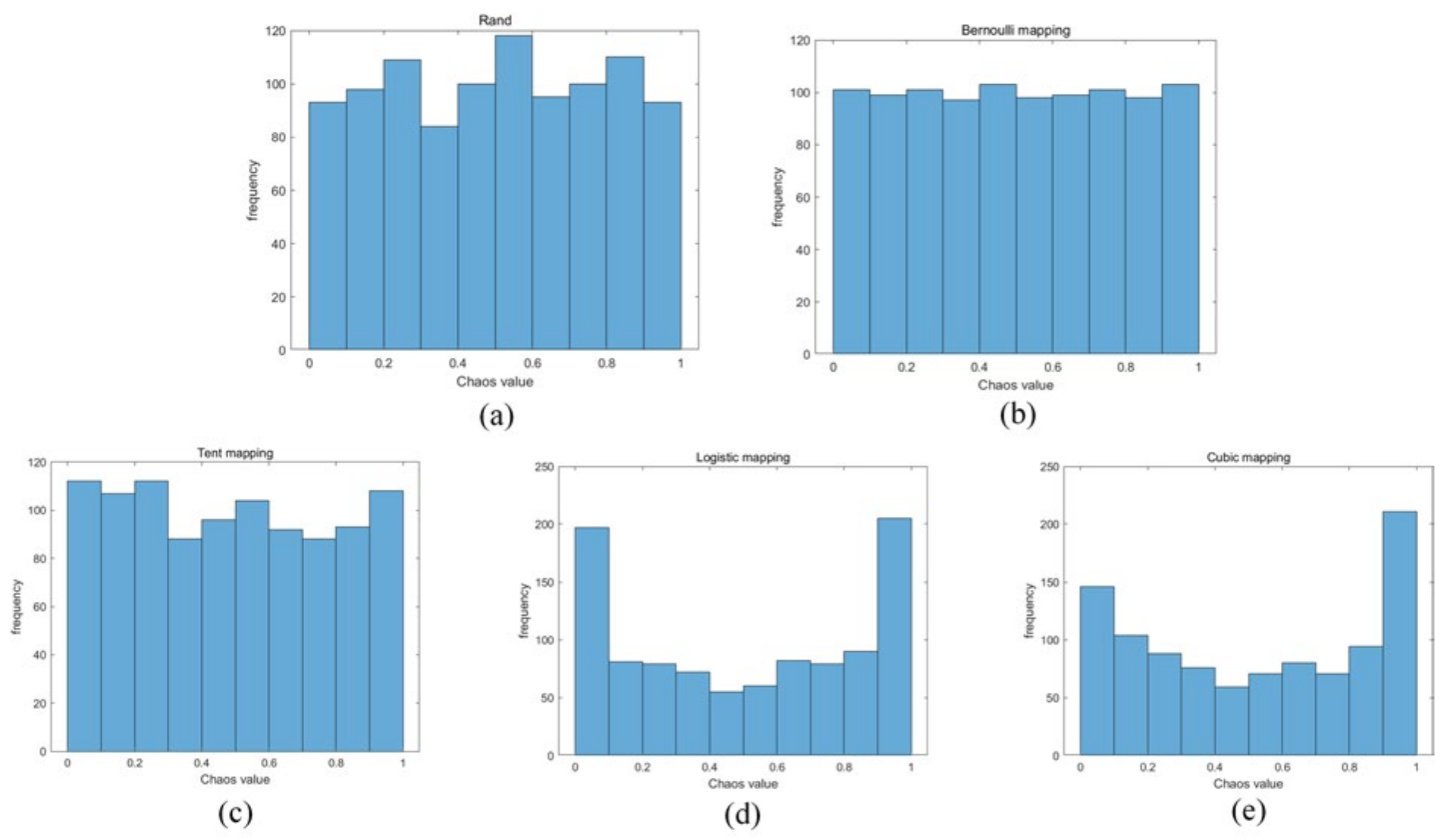
Currently, the most commonly used chaotic initialization methods include Bernoulli mapping, Logistic mapping, Tent mapping, and Cubic mapping. Figure 3 presents the frequency distribution histograms of random initialization compared to Bernoulli mapping, Logistic mapping, Tent mapping, and Cubic mapping. It can be observed that the distribution of Bernoulli mapping between the range of [0, 1] is more uniform compared to other chaotic mappings. Therefore, this paper introduces the Bernoulli mapping in the initialization stage of the MOAHA algorithm. The Bernoulli mapping is used to initialize the population, aiming to achieve a more uniform distribution of initial solutions in the solution space, thereby enhancing the quality and performance of the population and reducing the likelihood of falling into local optimal solutions. Bernoulli mapping is defined as follows:

$$x(t+1)=\left\{\begin{array}{l} \frac{x(t)}{1-\lambda }\hspace{1em}\hspace{1em},0<x(t)\le 1-\lambda \\ \frac{x(t)-1+\lambda }{\lambda }\hspace{1em},1-\lambda <x(t)<1\end{array}\right.$$

(23)

Assuming the population size is N, the population x = {x_i, i = 1,2,..., N} is obtained. where λ$\in$(0, 1) is a chaotic parameter, and in this paper, λ = 0.4 is adopted.

Figure 3. Histograms of random initialization and four types of chaotic mapping distributions. (a) Random Initialization. (b) Bernoulli mapping. (c) Tent mapping. (d) Logistic mapping. (e) Cubic mapping.

Figure 3. Histograms of random initialization and four types of chaotic mapping distributions. (a) Random Initialization. (b) Bernoulli mapping. (c) Tent mapping. (d) Logistic mapping. (e) Cubic mapping.

3.3. Adaptive Weights

The inertia weight factor is a crucial parameter. When the inertia weight is relatively large, the algorithm exhibits strong global search ability, increases population diversity, and can explore larger areas [27]. When the inertia weight is relatively small, the algorithm demonstrates strong local search ability and can finely explore the optimal solution, accelerating convergence speed. During local optimization, MOAHA utilizes territorial foraging and guided foraging for local search. When the hummingbird approaches the local optimal solution as described in (6) and (9), it can only obtain the local optimal solution and cannot achieve further local optimization. In response to this issue, this paper proposes a new adaptive weight method. When a hummingbird approaches food, a larger adaptive weight is used to adjust the optimal position of the hummingbird, thereby enhancing its local optimization ability. The adaptive weight formula is presented in Equation (17):

$$w=w_{\max }-(w_{\max }-w_{\min })\ast (\frac{e^{\frac{T_{\max }-t}{T_{\max }}}}{e-1}{)}^k$$

(24)

where w_min = 0.3, w_max = 0.8, t represents the current number of iteration cycles, while T_max specifies the upper limit of the maximum number of iteration cycles allowed for the entire optimization process.

Utilizing the adaptive weight Formula (17), (6) and (9) are enhanced, as demonstrated in Equations (18) and (19):

$$v_i(t+1)=w\ast x_{i,tr}(t)+a\ast D\ast (x_i(t)-x_{i,tr}(t))$$

(25)

$$\left\{\begin{array}{l}{v}_i(t+1)=w\ast x_i(t)+D\cdot b\cdot x_i(t)\hspace{1em}\hspace{1em}rand<0.5\\ v_i(t+1)=w\ast x_i(t)+D\cdot b\cdot x_a(t)\hspace{1em}\hspace{1em}rand\ge 0.5\end{array}\right.$$

(26)

By incorporating the adaptive weight factor w, each hummingbird possesses improved local optimization capabilities.

3.4. Dynamic Elimination Crowding Entropy

Unlike the single-objective artificial hummingbird optimization algorithm, MOAHA necessitates the establishment of an external archive to store non-inferior solutions. This paper utilizes entropy to depict the distribution of a solution along each objective in the objective function space. The distribution entropy of the i-th solution along the j-th objective function is defined as follows:

$$H_{ij}=-[p{l}_{ij}{\log }_2(p{l}_{ij})+p{u}_{ij}{\log }_2(p{u}_{ij})]$$

(27)

$$p{l}_{ij}=\frac{d{l}_{ij}}{c_{ij}}$$

(28)

$$p{u}_{ij}=\frac{d{u}_{ij}}{c_{ij}}$$

(29)

$$c_{ij}=d{l}_{ij}+d{u}_{ij}$$

(30)

where dl_ij and du_ij are the distances from the i-th solution along the j-th objective function to its adjacent solutions below and above. However, distribution entropy alone cannot accurately reflect the degree of congestion in the solution. To estimate the density of a solution in the objective function space, it is necessary to consider both crowding distance and distribution entropy simultaneously. Drawing from the above analysis and considering both crowding distance and distribution entropy, this paper introduces a new congestion evaluation method named Dynamic Elimination Congestion Entropy (DECE) to accurately measure congestion. This method eliminates the necessity to adjust the crowding entropy ranking of the remaining solutions after deleting one solution. DECE is defined as follows:

$$C{E}_i=\frac{{\displaystyle \sum _{j=1}^k(c_{ij}{E}_{ij})}}{\max (f_j)-\min (f_j)}=\frac{-{\displaystyle \sum _{j=1}^k(d{l}_{ij}{\log }_2(p{l}_{ij})+d{u}_{ij}{\log }_2(p{u}_{ij}))}}{\max (f_j)-\min (f_j)}$$

(31)

Before removing the i-th solution with the smallest current crowding distance, the distances between the previous and next solutions adjacent to the i-th solution are given as follows:

$$\left\{\begin{array}{l}d{l}_k(x_{i-1})=\left|f_k(x_{i-1})-f_k(x_{i-2})\right|\\ d{u}_k(x_{i-1})=\left|f_k(x_{i-1})-f_k(x_i)\right|\end{array}\right.$$

(32)

$$\left\{\begin{array}{l}d{l}_k(x_{i+1})=\left|f_k(x_{i+1})-f_k(x_i)\right|\\ d{u}_k(x_{i+1})=\left|f_k(x_{i+1})-f_k(x_{i+2})\right|\end{array}\right.$$

(33)

After removing the i-th solution with the smallest current crowding distance, the distances between the previous and next solutions adjacent to the i-th solution are given as follows:

$$\left\{\begin{array}{l}d{l}_k(x_{i-1})=\left|f_k(x_{i-1})-f_k(x_{i-2})\right|\\ d{u}_k(x_{i-1})=\left|f_k(x_{i-1})-f_k(x_{i+1})\right|\end{array}\right.$$

(34)

$$\left\{\begin{array}{l}d{l}_k(x_{i+1})=\left|f_k(x_{i+1})-f_k(x_{i-1})\right|\\ d{u}_k(x_{i+1})=\left|f_k(x_{i+1})-f_k(x_{i+2})\right|\end{array}\right.$$

(35)

Utilizing the new dl_ij and du_ij, the formula is updated, and the crowding entropy formula is calculated (24). During the iteration process, when the external archive is full, the external archive is maintained by calculating and eliminating the non-inferior solution with the minimum DECE. This approach serves to uphold population diversity and further accelerate the iteration speed.

3.5. Performance Comparison of Algorithms before and after Improvement

To ascertain the superiority of IMOAHA, it was compared with the MOAHA, MOGWO, MOPSO, and NSGA-II algorithms. The test functions ZDT1, ZDT2, and ZDT4 were selected, with a population of 100 and 500 iterations, and each algorithm was run 30 times. The evaluation of algorithm performance was conducted using the inverse generation distance (IGD), spacing index (SP), and hypervolume index (HV).

The IGD is an indicator used to evaluate the convergence and diversity performance of an algorithm. It represents the minimum distance between the non-dominated solution set that the algorithm has searched and the actual Pareto front. A smaller IGD value indicates better convergence and diversity of the algorithm. The calculation formula is as follows [28]:

$$IGD=\frac{{\displaystyle \sum \min \_d(x,PF)}}{\left|PF\right|}$$

(36)

where PF represents a set of uniformly distributed reference points sampled from the Pareto front.

The SP is an indicator used to evaluate algorithm diversity, representing the degree of uniformity of the distribution of non-dominated solutions obtained by the algorithm in the target space. A smaller SP value indicates a more uniform distribution of the target in space. The calculation formula is as follows [29]:

$$SP=\sqrt{\frac{1}{N-1}{\displaystyle \sum _{i=1}^N{(\overline{d}-d_i)}^2}}$$

(37)

where N represents the population size and d is the average value of d_i.

The HV is an indicator used to evaluate algorithm diversity and convergence, representing the volume of the region in the target space enclosed by the non-dominated solution set and reference points obtained by the algorithm. A larger HV value indicates better overall performance of the algorithm. The calculation formula is as follows [30]:

$$HV=\delta ({\displaystyle {\cup }_{i=1}^S{v}_i})$$

(38)

where S represents the non-dominated solution set calculated by the optimization algorithm and v_i represents the volume enclosed by the reference point and non-dominated solution set. The symbol δ(∙) denotes the Lebesgue measure used for calculating volume.

The comparison results of the optimization algorithms obtained using Matlab R2021b software are shown in

Table 3. Comparison results of optimization algorithms.

		IMOAHA	MOAHA	MOGWO	MOPSO	NSGII
ZDT1	IGD mean	1.9922 × 10−4	2.1192 × 10−4	1.4 × 10−3	5.9517 × 10−4	3.9 × 10−3
	IGD std	2.0248 × 10−6	5.51 × 10−6	5.1994 × 10−4	1.4133 × 10−4	4.8 × 10−3
	HV mean	7.205 × 10−1	7.194 × 10−1	7.027 × 10−1	7.057 × 10−1	6.194 × 10−1
	HV std	6.5023 × 10−5	3.0955 × 10−4	5.8 × 10−3	4.4 × 10−3	1.224 × 10−1
	SP mean	2.9 × 10−3	3.0 × 10−3	1.59 × 10−2	9 × 10−3	9.5 × 10−3
	SP std	2.7903 × 10−4	3.0767 × 10−4	5.1 × 10−3	1.2 × 10−3	9.9005 × 10−4
ZDT2	IGD mean	2.0444 × 10−4	2.1557 × 10−4	1.4 × 10−3	2.3921 × 10−4	8.7 × 10−3
	IGD std	2.6491 × 10−6	4.5518 × 10−6	4.7415 × 10−4	9.8751 × 10−6	1.01 × 10−1
	HV mean	4.451 × 10−1	4.439 × 10−1	4.220 × 10−1	4.431 × 10−1	2.801 × 10−1
	HV std	6.0386 × 10−5	3.5334 × 10−4	6.7 × 10−3	5.7408 × 10−4	1.752 × 10−1
	SP mean	2.9 × 10−3	3.0 × 10−3	1.40 × 10−2	6.7 × 10−3	1.02 × 10−1
	SP std	3.0328 × 10−4	2.7340 × 10−4	3.0 × 10−3	7.422 × 10−4	1.6 × 10−3
ZDT4	IGD mean	3.1637 × 10−4	3.3513 × 10−4	2.807 × 10−1	4.6726 × 10−4	4.097 × 10−1
	IGD std	4.7858 × 10−6	7.5150 × 10−6	1.731 × 10−1	5.8242 × 10−5	3.22 × 10−1
	HV mean	7.190 × 10−1	7.181 × 10−1	9.1 × 10−3	7.7173 × 10−1	8.3 × 10−3
	HV std	5.8521 × 10−5	1.4837 × 10−4	2.77 × 10−2	6.1118 × 10−4	3.16 × 10−2
	SP mean	3.0 × 10−3	3.1 × 10−3	3.029 × 10−1	8.8 × 10−3	5.022 × 10−1
	SP std	2.8363 × 10−4	3.9048 × 10−4	1.0960	1.7 × 10−3	1.0451
	IGD mean	1.9922 × 10−4	2.1192 × 10−4	1.4 × 10−3	5.9517 × 10−4	3.9 × 10−3

, indicating that the IMOAHA algorithm outperforms in terms of IGD, SP, and HV indicators. This demonstrates that IMOAHA exhibits superior convergence and diversity.

4. IPMSM Multi-Objective Optimization

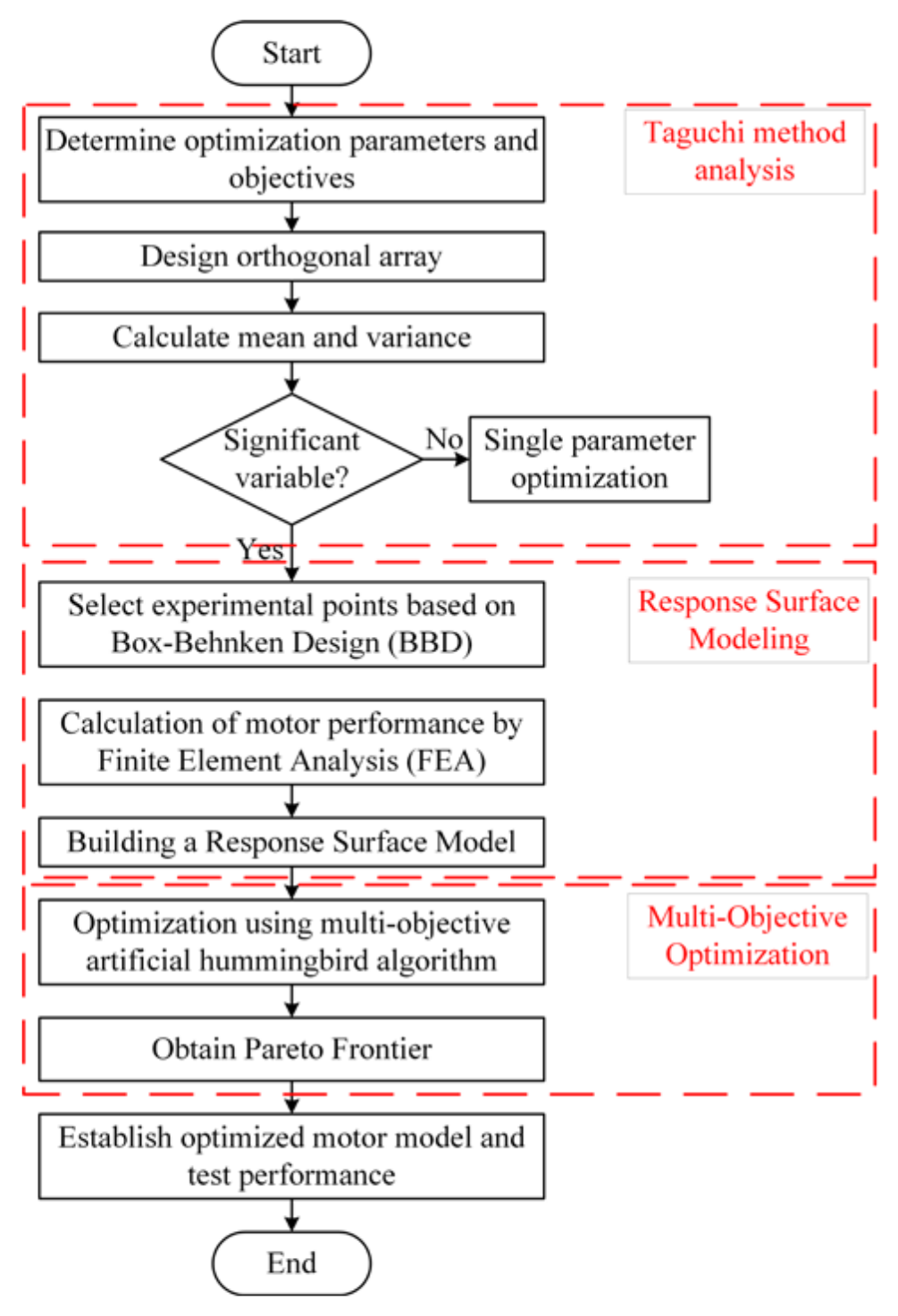
A multi-objective optimization problem refers to the simultaneous existence of multiple objectives that require optimization, taking into account their mutual influence. Multi-objective optimization may have one or more solutions, which are the optimal solutions determined after considering various optimization objectives. The specific optimization of IPMSM mainly consists of four steps: determination of optimization objectives and parameters, the Taguchi method, response surface modeling, and IMOAHA optimization. The process diagram for multi-objective optimization design is illustrated in Figure 4.

4.1. Optimization Objectives and Parameter Determination

To attain higher operational stability, lower noise, and increased torque for IPMSM, the optimization objectives of average torque (T_avg), torque ripple (T_ripple), EMF, and iron loss (P_fe) were established. As illustrated in Figure 1b, the mounting location of the permanent magnet within the motor rotor core is contingent upon the dimensions of Wh_y, Rib_y, Rib_v, and HRib_v. Alterations in the utilization and positioning of permanent magnets may result in modifications to the distribution of magnetic field strength within the motor, consequently influencing the output torque performance of the motor. The dimensions of each slot in the stator core are primarily dictated by B_s1 and H_s2. Variations in B_s1 and H_s2 can influence the magnetic field distribution of the stator teeth and yoke, thereby exerting a notable impact on iron loss during motor operation.

In addition to the aforementioned six parameters, there are additional factors that require consideration, including the stator tooth width (w_t), the separation between V-shaped and I-shaped permanent magnets, and the distance between V-shaped permanent magnets and shafts. B_s1 denotes the stator tooth width, while HRib_v signifies the distance between V-shaped and I-shaped permanent magnets. Hence, the impact of Bs1 and HRibv on motor performance can supplant the effects of stator tooth width and the distance d between V-shaped and I-shaped permanent magnets on motor performance. Certain parameters exhibit a relatively minor influence on the optimization objective. Based on preliminary experimental validation, as depicted in Figure 5, the distance between the V-shaped permanent magnet and the shaft, as well as the distance between the V-shaped permanent magnet and the side magnet, demonstrate a relatively negligible impact on the optimization objective.

Drawing on the analysis above, the structural parameters of Wh_y, Rib_y, Rib_v, HRib_v, B_s1, and H_s2 have been chosen as the variables for this optimization. To fulfill the performance criteria for optimizing IPMSM, particular constraints need to be imposed on the optimized entity. The multi-objective optimization problem and constraint conditions outlined in this study can be formulated as follows:

$$\min \left\{\begin{array}{l}1/T_{avg}\\ T_{ripple}\\ EMF\\ P_{fe}\end{array}\right.$$

(39)

$$s.t.\left\{\begin{array}{l}{T}_{avg}\ge 55N\cdot m\\ T_{ripple}\le 8\%\end{array}\right.$$

(40)

4.2. Optimization of The Taguchi Method

The Taguchi method is a local optimization approach that can concurrently optimize multiple motor performance parameters, offering the advantages of reduced testing, lower cost, and shorter design cycles [8]. By utilizing orthogonal experimental design, it enables saving on design time and cost, facilitating the identification of the optimal parameter combination within the shortest possible timeframe. Additionally, the Taguchi method can mitigate the impact of various noise factors. The levels of each optimization factor are detailed in

Table 4. Optimization factor levels.

Optimization Factor	Level 1	Level 2	Level 3	Level 4	Level 5
Slot body height Hs2/mm	24.6	24.85	25.1	25.35	25.6
Slot wedge maximum width Bs1/mm	3.6	3.95	4.3	4.65	5
Rib width of 1-shaped PM Riby/mm	19	19.5	20	20.5	21
Width of 1-shaped PM Why/mm	30	31	32	33	34
Rib width of V-shaped PM Ribv/mm	1	1.5	2	2.5	3
Rib height of V-shaped PM HRibv/mm	3	3.5	4	4.5	5

.

An L25 experimental orthogonal table will be established based on the number of optimization parameters selected in Table 4 and the level of their values. This design requires only 25 experiments to achieve optimization goals, significantly reducing computational complexity and the number of experiments. The finite element model in Maxwell 2021R1 software will be used to simulate and analyze the four optimization objectives for each experiment. The finite element simulation results are shown in

Table 5. Finite element simulation results.

Test Number	Test Matrix						Tavg/N·m	Tripple/N·m	EMF/V	Pfe/W
	Bs1	HRibv	Hs2	Ribv	Riby	Why
1	1	1	1	1	1	1	55.11	8.05	428.01	235.87
2	1	2	2	2	2	2	56.97	8.24	434.67	258.01
3	1	3	3	3	3	3	58.74	6.81	446.91	267.58
4	1	4	4	4	4	4	60.14	6.29	459.29	265.87
5	1	5	5	5	5	5	60.83	7.30	472.25	270.47
6	2	1	2	3	4	5	59.67	5.74	448.14	250.1
7	2	2	3	4	5	1	57.84	10.47	458.7	254.44
8	2	3	4	5	1	2	57.44	5.97	458.43	270.51
9	2	4	5	1	2	3	57.16	9.24	431.89	250.49
10	2	5	1	2	3	4	60.14	9.8	450.48	260.25
11	3	1	3	5	2	4	58.61	6.66	456.08	251.87
12	3	2	4	1	3	5	58.08	9.48	432.44	237.48
13	3	3	5	2	4	1	56.01	11.7	436.32	229.35
14	3	4	1	3	5	2	59	12.16	449.34	248.57
15	3	5	2	4	1	3	58.79	4.87	443.82	258.69
16	4	1	4	2	5	3	57.18	11.26	429	221.52
17	4	2	5	3	1	4	56.58	4.82	429.62	243.23
18	4	3	1	4	2	5	59.44	7.55	450.48	248.07
19	4	4	2	5	3	1	57.56	8.67	446.13	240.31
20	4	5	3	1	4	2	57.32	13.15	429.35	239.54
21	5	1	5	4	3	2	55.8	7.4	430.51	228.3
22	5	2	1	5	4	3	58.54	6.34	445.73	220.7
23	5	3	2	1	5	4	58.02	14.09	436.32	229.35
24	5	4	3	2	1	5	57.64	10.71	446.34	236.82
25	5	5	4	3	2	1	55.65	10.5	415.11	236.49

.

In order to analyze the impact and proportion of parameter changes in motor optimization factors on optimization objectives, a statistical analysis of the experimental data was conducted based on the established orthogonal experimental table and the finite element analysis results presented in Table 5. To determine the proportion of the impact of all optimization factors on each optimization objective, mean analysis and variance analysis were conducted.

First, the average finite element simulation results of various optimization objectives were calculated according to Equation (34), and the results are shown in

Table 6. Average results of various optimization goals.

	Tavg/N·m	Tripple/N·m	EMF/V	Pfe/W
m	57.93	8.69	442.61	246.15

.

$$m=\frac{1}{n}{\displaystyle \sum _{i=1}^n{P}_i}$$

(41)

where m is the average value of the experiment, N is the number of experiments, and P_i is the optimization objective value for the i-th time.

Subsequently, the average simulation analysis of a specific performance indicator of the motor corresponding to changes in each optimization factor was conducted. According to Equation (35), the average values of the optimization factor at different levels were calculated and the results are presented in

Table 7. Average values of motor performance indicators for various optimization factors at different levels.

Optimization Factor	Level	Tavg/N·m	Tripple/N·m	EMF/V	Pfe/W
Bs1	1	58.36	7.34	448.22	259.56
	2	58.45	8.24	449.53	257.16
	3	58.10	8.97	443.60	245.19
	4	57.62	9.09	436.91	238.53
	5	57.13	9.81	434.80	230.33
HRibv	1	57.93	8.69	442.61	246.15
	2	57.60	7.87	440.23	242.77
	3	57.93	9.22	445.69	248.97
	4	58.30	9.41	446.60	248.41
	5	58.55	9.12	442.20	253.09
Hs2	1	58.45	8.78	444.81	242.69
	2	58.20	8.32	441.81	247.29
	3	58.03	9.56	447.48	250.05
	4	57.70	8.70	438.85	246.37
	5	57.28	8.09	440.12	244.37
Ribv	1	57.14	10.80	431.60	238.54
	2	57.59	10.34	439.36	241.19
	3	57.93	8.01	437.82	249.19
	4	58.40	7.32	448.56	251.07
	5	58.60	6.99	455.72	250.77
Riby	1	57.11	6.88	441.24	249.02
	2	57.57	8.44	437.64	248.98
	3	58.06	8.43	441.29	246.78
	4	58.34	8.64	443.77	241.11
	5	58.57	11.05	449.12	244.87
Why	1	56.43	9.88	436.85	239.29
	2	57.31	9.38	440.46	248.99
	3	58.08	7.70	439.47	243.80
	4	58.70	8.33	446.36	250.11
	5	59.13	8.16	449.93	248.59

.

$$m_{T_{avg}}(B_{s11})=\frac{1}{5}(T_{avg}(1)+T_{avg}(2)+T_{avg}(3)+T_{avg}(4)+T_{avg}(5))$$

(42)

The proportion of the impact of each optimization parameter on the optimization objective was calculated based on Table 6 and Table 7. The formula is shown in Equation (36) and the results are presented in

Table 8. The proportion of each optimization parameter for each performance indicator.

Optimization Factor	Tavg/N·m		Tripple/N·m		EMF/V		Pfe/W
	STavg	Proportion (%)	STripple	Proportion (%)	SEMF	Proportion (%)	SPfe	Proportion (%)
Bs1	0.24	0.12	0.70	0.11	34.75	0.22	122.04	0.62
HRibv	0.13	0.06	0.33	0.05	6.24	0.04	14.50	0.07
Hs2	0.17	0.08	0.25	0.04	9.89	0.06	6.34	0.03
Ribv	0.28	0.14	2.49	0.40	72.39	0.45	27.45	0.14
Riby	0.28	0.14	1.80	0.29	14.41	0.09	8.75	0.04
Why	0.94	0.46	0.65	0.11	23.05	0.14	16.45	0.08
Total	2.04	1.00	6.23	1.00	160.72	1.00	195.53	1.00

.

$$S=\frac{1}{n}{\displaystyle \sum _{i=1}^n{(m_{x_i}(P)-m(P))}^2}$$

(43)

where x is the optimization factor, P denotes the optimization objective, m(P) signifies the average value of the optimization objective, m_xi(P) represents the average value of the optimization factor x at level i, S denotes the variance, and n represents the number of levels of each optimization factor.

In Table 8, the proportion of S values for each optimization parameter under the corresponding optimization objective reflects the impact of the optimization parameter on the optimization objective. It is evident that altering the parameter B_s1 has the most significant impact on the iron loss P_fe while changing the parameters Rib_v, Rib_y, and Wh_y has the greatest impact on the average torque T_avg. Additionally, adjusting the parameters Rib_v and Rib_y has the most substantial impact on the torque ripple T_ripple, and modifying the parameter Rib_v has the greatest impact on the back EMF. Consequently, for subsequent analysis, four optimization parameters, namely B_s1, Rib_y, Wh_y, and Rib_v, were selected.

4.3. Response Surface Modeling

The fundamental concept of the response surface model is to construct a polynomial function based on the system’s response at a series of sampling points to approximate an implicit function [31]. As experimental response values were not obtainable during the design phase, finite element simulation results were used as the system response to establish mathematical models between various optimization parameters and optimization objectives. This paper adopts the second-order polynomial regression method to establish a response surface model, which takes the following form:

$$Y={\beta }_0+{\displaystyle \sum _{i=1}^n{\beta }_i{x}_i}+{\displaystyle \sum _{i=j}^n{\beta }_{ii}{x}_i^2}+{\displaystyle \sum _{i\ne j}^n{\beta }_{ij}{x}_i{x}_j+\epsilon }$$

(44)

where Y represents the optimization objective; β₀ is a constant term; β_i, β_ij, and β_ii are the first-order and second-order coefficients of the optimization parameters; x_i and x_j are different optimization parameters; and ε denotes a random error.

A variety of experimental design methods are available for constructing response surface models, and the Box–Behnken design (BBD) method utilized in this paper is a classic and commonly employed experimental design approach. This method is suitable for establishing response surface models containing 2–5 factors. In the BBD method, each factor has three levels, namely −1, 0, and 1, where 0 represents the center point, while 1 and −1 correspond to the maximum and minimum values, respectively. The levels of significant variables analyzed using the Taguchi method are shown in

Table 9. Significant variable levels.

Parameter	−1	0	1
Bs1/mm	3.6	4.3	5
Riby/mm	19	20	21
Why/mm	30	32	34
Ribv/mm	1	2	3

.

Using finite element simulation software for experiments, 29 sets of experiments are required according to the Box–Behnken design method due to the existence of four optimization parameters. By analyzing the resulting data using Design Expert 13 software, the multi-objective optimization function is obtained as follows:

$$\begin{array}{l}{T}_{avg}=57.00-0.74\times B_{s1}+0.79\times Ri{b}_v+0.74\times Ri{b}_y+1.38\times W{h}_y+0.19\times B_{s1}\times Ri{b}_v\\ +0.023\times B_{s1}\times Ri{b}_y-0.022\times B_{s1}\times W{h}_y-0.014\times Ri{b}_v\times Ri{b}_y-0.046\times Ri{b}_v\times W{h}_y\\ -0.121\times Ri{b}_y\times W{h}_y-0.026\times B_{s1}^2+0.2001\times Ri{b}_v^2+0.034\times Ri{b}_y^2-0.119\times W{h}_y^2\end{array}$$

(45)

$$\begin{array}{l}{T}_{ripple}=6.33-0.702\times B_{s1}-2.03\times Ri{b}_v+1.31\times Ri{b}_y-1.41\times W{h}_y-0.87\times B_{s1}\times Ri{b}_v\\ +0.47\times B_{s1}\times Ri{b}_y+0.29\times B_{s1}\times W{h}_y-0.73\times Ri{b}_v\times Ri{b}_y-0.06\times Ri{b}_v\times W{h}_y\\ -0.95\times Ri{b}_y\times W{h}_y+0.76\times B_{s1}^2+0.97\times Ri{b}_v^2+0.9\times W{h}_y^2\end{array}$$

(46)

$$\begin{array}{l}EMF=422.03-8.86\times B_{s1}+13.97\times Ri{b}_v+5.74\times Ri{b}_y+6.04\times W{h}_y-1.15\times B_{s1}\times Ri{b}_v\\ -6.10\times B_{s1}\times Ri{b}_y+6.49\times B_{s1}\times W{h}_y+0.77\times Ri{b}_v\times Ri{b}_y-1.34\times Ri{b}_v\times W{h}_y\\ -3.34\times Ri{b}_y\times W{h}_y+6.60\times B_{s1}^2+9.96\times Ri{b}_v^2+9.07\times Ri{b}_y^2+6.64\times W{h}_y^2\end{array}$$

(47)

$$\begin{array}{l}{P}_{fe}=248.66-18.15\times B_{s1}+7.35\times Ri{b}_v-4.66\times Ri{b}_y-0.37\times W{h}_y-4.95\times B_{s1}\times Ri{b}_v\\ -3.26\times B_{s1}\times Ri{b}_y-1.52\times B_{s1}\times W{h}_y-2.75\times Ri{b}_v\times Ri{b}_y-1.56\times Ri{b}_v\times W{h}_y\\ -1.43\times Ri{b}_y\times W{h}_y-2.55\times B_{s1}^2-2.83\times Ri{b}_v^2-2.04\times Ri{b}_y^2-0.72\times W{h}_y^2\end{array}$$

(48)

Through significance testing and analysis of variance in Design Expert software, the regression equations for the four optimization objectives were further analyzed. The evaluation of the objective model is presented in

Table 10. Response surface method analysis results.

Optimization Objectives	p Value	R2
Tavg	<0.0001	0.9801
Tripple	<0.0001	0.9247
EMF	<0.0001	0.9184
Pfe	<0.0001	0.9837

. The degree of approximation of IPMSM performance and the response surface model is represented by the multiple correlation coefficient R². An R² value close to 1 indicates a more accurate model.

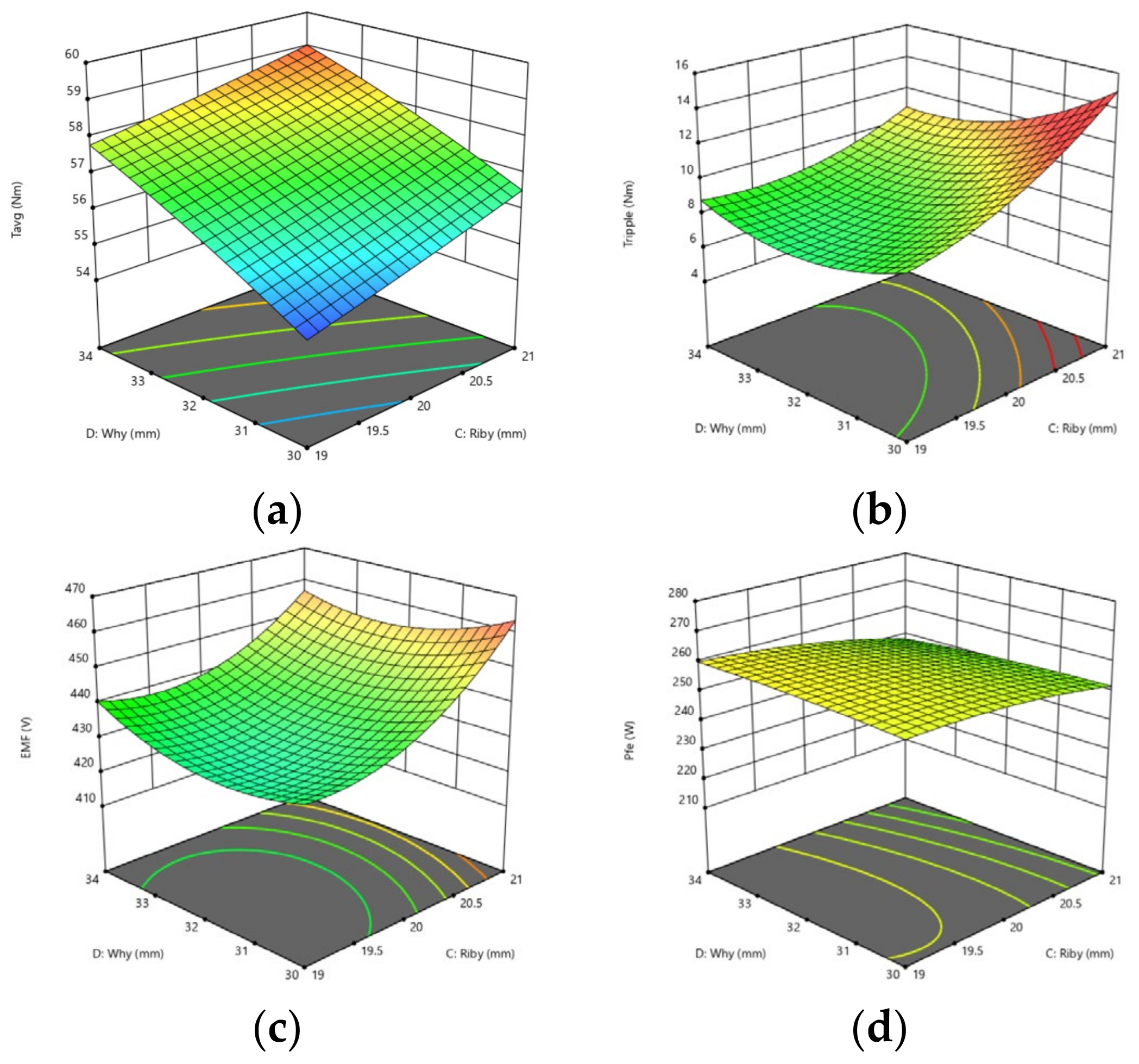
Based on the analysis in Table 10, it is observed that the R² values of the four models are all higher than 0.9, indicating good applicability and strong correlation. The response surface of the optimization objective for the optimization parameters is depicted in Figure 6. It is evident that the response surface model exhibits extreme values, and the optimization parameters also have an optimal range. However, the optimal value range corresponding to each response surface model is not the same. Hence, to mitigate conflicts between design objectives, it is essential to employ multi-objective intelligent optimization algorithms to attain the Pareto optimal solution for multi-objective optimization problems.

4.4. IMOAHA Optimization Results

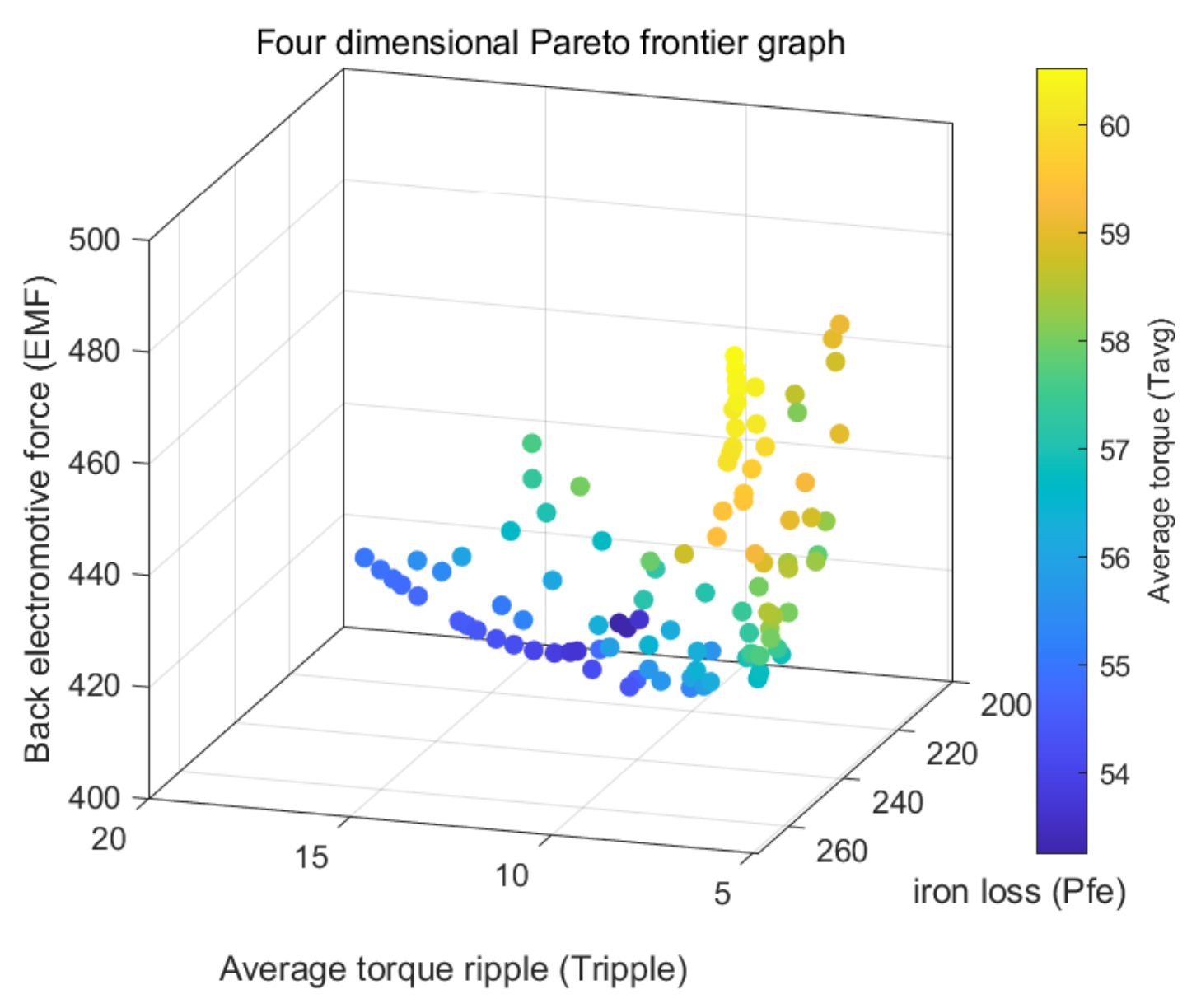
The IMOAHA algorithm introduced in Section 2 is designed in MATLAB and sets the population size and external file to 100 and the number of iterations to 500. The regression equation obtained by the response surface method is optimized and the program is run to obtain the Pareto frontier shown in Figure 7.

In Figure 7, the color of the spheres in the figure indicates the average torque magnitude, where yellow denotes the high average torque value and blue signifies the low average torque value. Considering the performance of IPMSM holistically, the optimal solution for IPMSM was chosen from the four-dimensional Pareto solution set, yielding the optimized parameters for IPMSM under this solution.

5. Simulation Experiment

5.1. Analysis of Simulation Results

IPMSM 2D models before and after optimization are built in Maxwell 2021R1 FEA software, and the performance is compared and analyzed. Since the size of the mesh and the time step are both factors that affect the calculation time of the finite element model in finite element analysis, this paper divides the permanent magnet mesh into 1 mm, the rotor meshes into 2 mm, the stator meshes into 3 mm, and the time step is set to 5 × 10⁻⁵ s. At this time, the calculation time of the finite element is 200 s. The values of motor optimization variables before and after optimization are given in

Table 11. Comparison between optimization parameters and optimization objectives.

Parameter	Before Optimization	After Optimization
Hs2/mm	25.6	24.6
Bs1/mm	3.6	5
Riby/mm	21	19
Why/mm	30	32
Ribv/mm	1	3
HRibv/mm	5	3.5
Tavg/N·m	57.1185	57.3069
Tripple/%	12.9758	3.5331
EMF/V	457.0765	435.7698
Pfe/W	266.3347	242.3543

. The finite element simulation results are shown from Figure 8, Figure 9, Figure 10 and Figure 11.

According to Table 11, reducing the width of the magnetic barrier through optimization decreases magnetic leakage, resulting in an overall improvement in the performance of the motor.

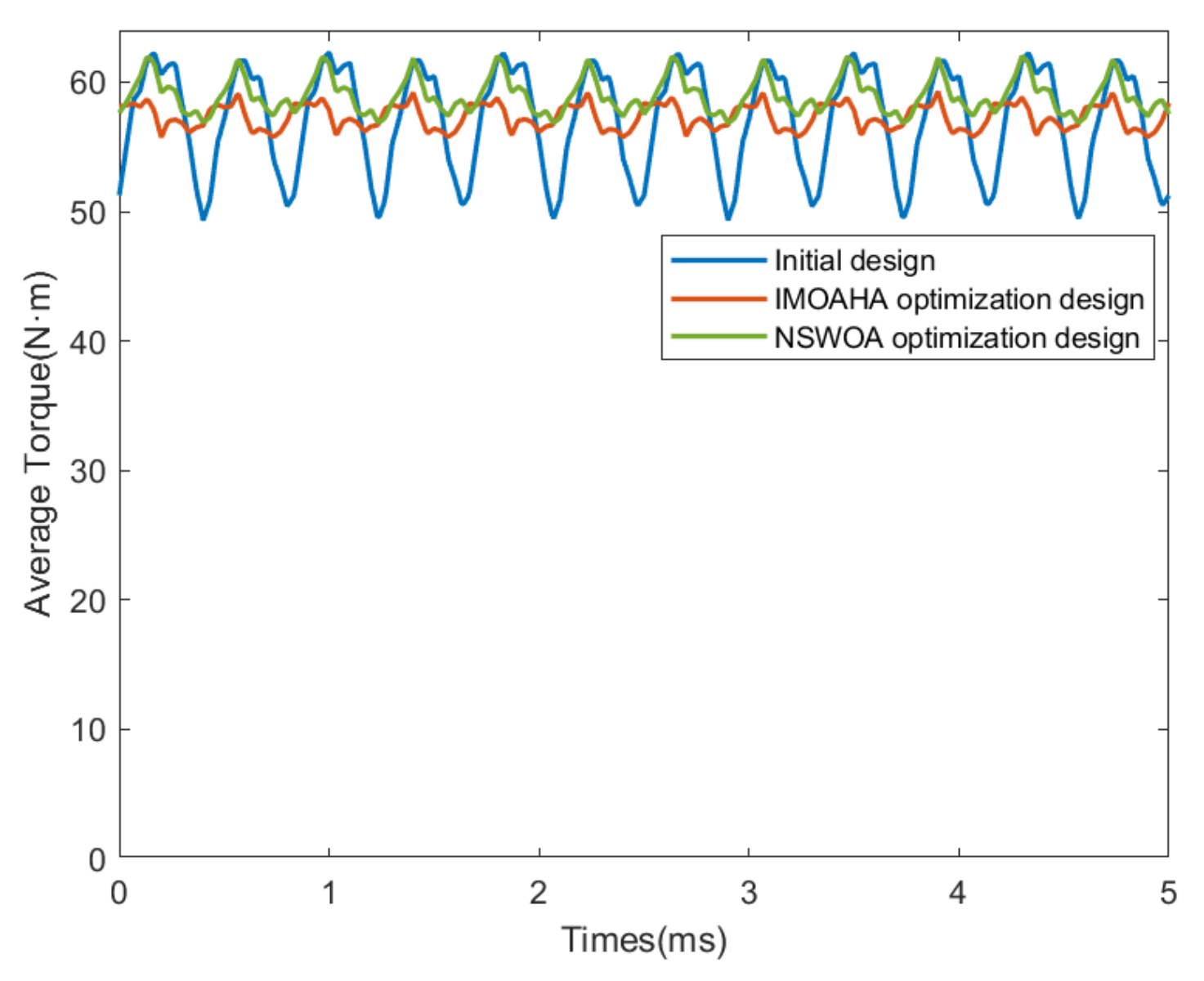
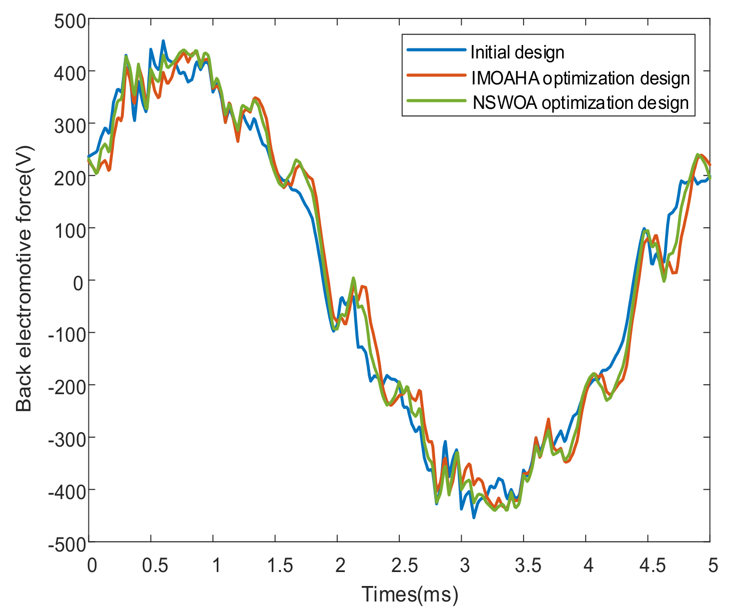
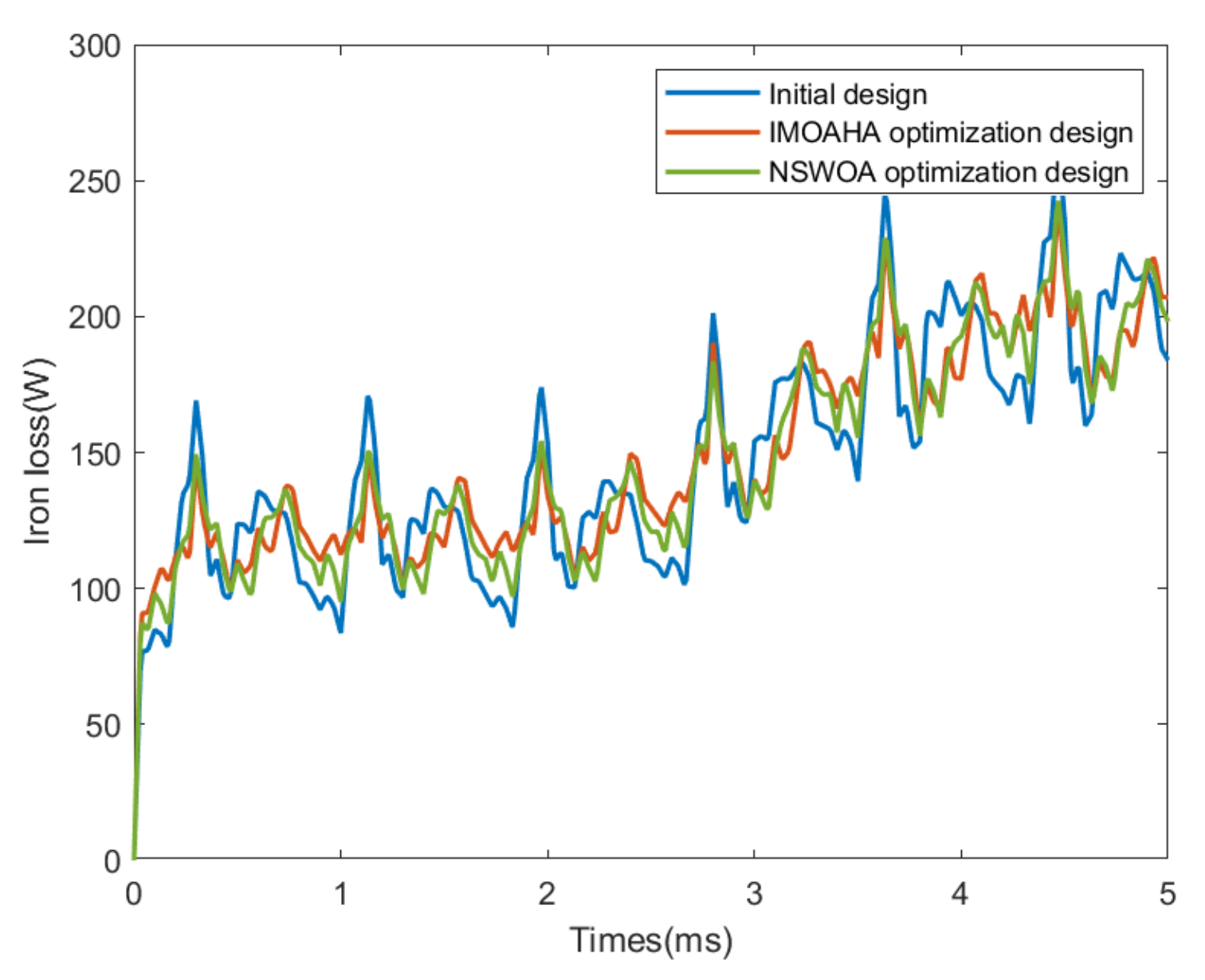
Figure 8 shows the comparison of torque performance before and after optimization. Compared to the initial design, the average torque of the motor increased by 0.33% after optimization, and the torque ripple decreased by 72.77%. Figure 9 and Figure 10 depict the comparison of back electromotive force and iron core loss before and after optimization. Following optimization, the back electromotive force decreased by 4.66% and the iron core loss decreased by 9.01% compared to the initial design. Figure 11 indicates that at rated speed, the efficiency of the IPMSM can reach 97%. The efficiency of the permanent magnet synchronous motor before optimization is 97.01%, and the efficiency of the permanent magnet synchronous motor after optimization is 97.18%. Therefore, the efficiency increase of the permanent magnet synchronous motor after and before optimization is not significant.

A comparison of results demonstrates that the multi-objective optimization design, utilizing the Taguchi method in combination with the IMOAHA algorithm, effectively reduces torque ripple and iron core loss while also improving torque and motor efficiency. This success indicates the feasibility and effectiveness of optimizing IPMSM parameters using the Taguchi method and IMOAHA, highlighting the comprehensive nature of this approach in achieving performance enhancements across multiple key metrics.

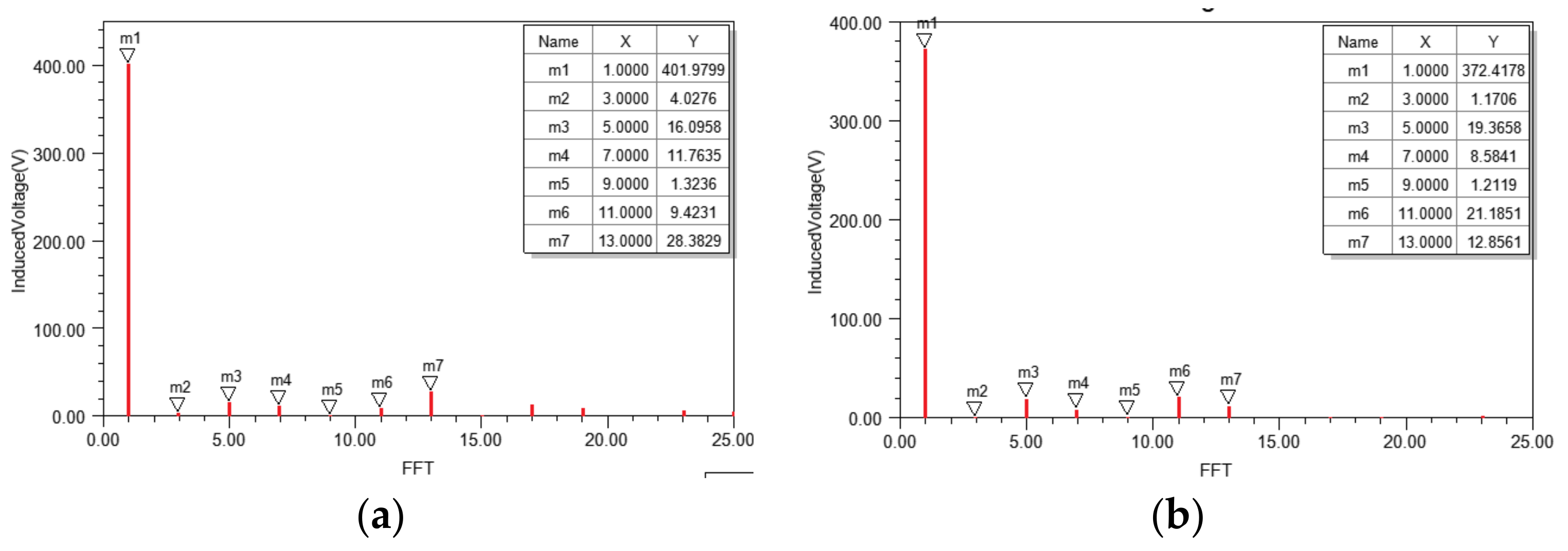
Based on the Fourier decomposition of the back electromotive force before and after optimization, the harmonic values of the back electromotive force before and after optimization can be obtained. From Figure 12, it can be seen that the harmonic values after optimization are reduced. The larger the harmonic of the back electromotive force, the greater the iron loss [32]. Therefore, due to the reduction in the harmonic of the back electromotive force, the iron loss also decreases.

To validate the effectiveness of the enhanced multi-objective artificial hummingbird algorithm, the non-dominated sorting whale optimization algorithm (NSWOA) [33] was employed to optimize the parameters of the internal permanent magnet synchronous motor design. Subsequently, the motor’s performance was evaluated and the comparative outcomes are presented in Figure 8, Figure 9 and Figure 10. Figure 8 reveals that the torque fluctuation of the permanent magnet synchronous motor optimized by the non-dominated sorting whale optimization algorithm is more pronounced and exhibits larger vibrations compared to that optimized by the improved multi-objective artificial hummingbird algorithm. Figure 9 and Figure 10 indicate that the back electromotive force and core loss of the NSWOA-optimized permanent magnet synchronous motor exhibit minimal changes in contrast to the IMOAHA-optimized back electromotive force and core loss. The back electromotive force increases by 1.38% and the core loss increases by 0.82%. Thus, the performance of the motor optimized by the Improved Multi-Objective Artificial Hummingbird Algorithm surpasses that of the motor optimized by the Non-dominated Sorting Whale Optimization Algorithm.

5.2. Simulink Experimental Verification

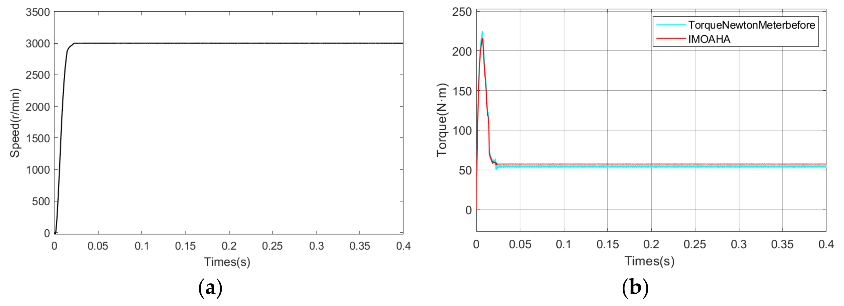
To validate the efficacy of the proposed optimization algorithm, an Internal Permanent Magnet Synchronous Motor (IPMSM) simulation control system was developed in the Matlab/Simulink environment. Initially, a motor load start simulation was performed, with Figure 13a,b illustrating the IPMSM speed waveform and torque waveform, respectively. The complete startup sequence of the IPMSM lasted 0.02 s, leading to stable operation at a speed of 3000 r/min, characterized by minimal overshoot throughout the initiation phase. After startup completion, torque variations occurred, with the torque fluctuation of the original motor markedly exceeding that of the IPMSM optimized through the enhanced multi-objective artificial hummingbird algorithm. The simulation experiment findings indicate that the internal permanent magnet synchronous motor, enhanced by the optimization algorithm, exhibits enhanced stability, thereby validating the efficacy of the optimization algorithm for motor enhancement.

6. Conclusions

This paper presents enhancements to the multi-objective artificial hummingbird algorithm through the incorporation of an adaptive weight method, chaotic mapping, and dynamic crowding entropy. Additionally, it proposes a novel multi-objective optimization design that combines the Taguchi method with the improved multi-objective artificial hummingbird algorithm, thereby offering a comprehensive optimization approach. Firstly, an orthogonal experimental design is conducted on the selected six parameters, utilizing the Taguchi method to identify the parameters significantly impacting the optimization objective. Secondly, a response surface model is employed to analyze the parameters and formulate the equation for the optimization objective function. Subsequently, the improved MOAHA algorithm is utilized to optimize the parameters and obtain the optimal combination. Finally, the optimization results are validated using a finite element model. The results demonstrate that the multi-objective optimization design, combining the Taguchi method and IMOAHA algorithm, effectively overcomes the limitations of single-objective algorithms, while exhibiting high optimization efficiency. The application of the optimized permanent magnet synchronous motor in this paper can serve as a driving motor for new energy vehicles, providing high power density, improving passenger comfort, and reducing vehicle noise.

The approach presented in this article is universally applicable to all configurations of permanent magnet synchronous motors. The core concept of this methodology is to provide optimization parameters and their corresponding objective functions, thereby deriving the optimized results. Consequently, by offering optimization parameters and objective functions, this method can compute the optimized results for any configuration of a permanent magnet synchronous motor.

References

1. Chu, J.; Cheng, H.; Sun, J.; Peng, C.; Hu, Y. Multi-objective optimization design of hybrid excitation double stator permanent magnet synchronous machine. J. IEEE Trans. Energy Convers. 2023, 38, 2364–2375. [Google Scholar] [CrossRef]
2. Sindhya, K.; Manninen, A.; Miettinen, K.; Pippuri, J. Design of a permanent magnet synchronous generator using interactive multiobjective optimization. J. IEEE Trans. Ind. Electron. 2017, 64, 9776–9783. [Google Scholar] [CrossRef]
3. Shen, J.; Chen, X.; Cui, Z.; Ma, L. Optimization design and research on vibration and noise of permanent magnet synchronous motor for vehicle. Prog. Electromagn. Res. M 2021, 100, 105–115. [Google Scholar] [CrossRef]
4. Lee, S.J.; Kim, K.S.; Cho, S.; Jang, J.; Lee, T.H.; Hong, J.P. Optimal design of the magnetizing fixture using Taguchi robust design in the ring-type PMSM. In Proceedings of the 7th IET International Conference on Power Electronics, Machines and Drives (PEMD 2014), Manchester, UK, 8–10 April 2014; pp. 1–6. [Google Scholar]
5. Wu, S.; Pang, X.; Tong, W.; Yao, Y. Design of rotor magnetic barrier structure of built-in permanent magnet motor based on taguchi method. CES Trans. Electr. Mach. Syst. 2023, 7, 193–201. [Google Scholar] [CrossRef]
6. Lai, C.; Feng, G.; Iyer, K.L.V.; Mukherjee, K.; Kar, N.C. Genetic algorithm-based current optimization for torque ripple reduction of interior PMSMs. EEE Trans. Ind. Appl. 2017, 53, 4493–4503. [Google Scholar] [CrossRef]
7. Coello, C.A.C.; Pulido, G.T.; Lechuga, M.S. Handling multiple objectives with particle swarm optimization. EEE Trans. Evol. Comput. 2004, 8, 256–279. [Google Scholar] [CrossRef]
8. Deb, K.; Pratap, A.; Agarwal, S.; Meyarivan, T.A.M.T. A fast and elitist multiobjective genetic algorithm: NSGA-II. IEEE Trans. Evol. Comput. 2002, 6, 182–197. [Google Scholar] [CrossRef]
9. Mirjalili, S.; Saremi, S.; Mirjalili, S.M.; Coelho, L.D.S. Multi-objective grey wolf optimizer: A novel algorithm for multi-criterion optimization. Expert Syst. Appl. 2016, 47, 106–119. [Google Scholar] [CrossRef]
10. Von Lücken, C.; Barán, B.; Brizuela, C. A survey on multi-objective evolutionary algorithms for many-objective problems. Comput. Optim. Appl. 2014, 58, 707–756. [Google Scholar] [CrossRef]
11. Yang, X.S.; Deb, S. Multiobjective cuckoo search for design optimization. Comput. Oper. Res. 2013, 40, 1616–1624. [Google Scholar] [CrossRef]
12. Zhao, W.; Zhang, Z.; Mirjalili, S.; Wang, L.; Khodadadi, N.; Mirjalili, S.M. An effective multi-objective artificial hummingbird algorithm with dynamic elimination-based crowding distance for solving engineering design problems. Comput. Methods Appl. Mech. Eng. 2022, 398, 115223. [Google Scholar] [CrossRef]
13. Xu, R.; Tong, W. Multi-objective Hierarchical Optimization of Interior Permanent Magnet Synchronous Machines Based on Rotor Surface Modification. CES Trans. Electr. Mach. Syst. 2022, 6, 352–358. [Google Scholar] [CrossRef]
14. Sun, K.; Tian, S. Multiobjective optimization of IPMSM with FSCW applying rotor notch design for torque performance improvement. IEEE Trans. Magn. 2022, 58, 8104909. [Google Scholar] [CrossRef]
15. Hong, G.; Wei, T.; Ding, X. Multi-objective optimal design of permanent magnet synchronous motor for high efficiency and high dynamic performance. IEEE Access 2018, 6, 23568–23581. [Google Scholar] [CrossRef]
16. Liu, G.; Wang, Y.; Chen, Q.; Xu, G.; Song, C. Multiobjective deterministic and robust optimization design of a new spoke-type permanent magnet machine for the improvement of torque performance. IEEE Trans. Ind. Electron. 2020, 67, 10202–10212. [Google Scholar] [CrossRef]
17. Qu, C.; Guo, Z.; Hu, Y.; Wang, X.; Han, F. Multi-Objective Optimization Design of a New Permanent Magnet Synchronous Motor Based on the Taguchi Method. Energies 2022, 15, 7347. [Google Scholar] [CrossRef]
18. Liu, X.; Peng, W.; Xie, L.; Zhang, X. Optimization of a Multi-Type PMSM Based on Pyramid Neural Network. Appl. Sci. 2023, 13, 6810. [Google Scholar] [CrossRef]
19. Baek, S.-W.; Lee, S.W. Design Optimization and Experimental Verification of Permanent Magnet Synchronous Motor Used in Electric Compressors in Electric Vehicles. Appl. Sci. 2020, 10, 3235. [Google Scholar] [CrossRef]
20. Hua, Y.; Zhu, H.; Gao, M.; Ji, Z. Multiobjective optimization design of permanent magnet assisted bearingless synchronous reluctance motor using NSGA-II. IEEE Trans. Ind. Electron. 2020, 68, 10477–10487. [Google Scholar] [CrossRef]
21. Ahmadi, S.; Lubin, T.; Vahedi, A.; Taghavi, N. Sensitivity-Based Optimization of Interior Permanent Magnet Synchronous Motor for Torque Characteristic Enhancement. Energies 2021, 14, 2240. [Google Scholar] [CrossRef]
22. Sato, H.; Igarashi, H. Deep learning-based surrogate model for fast multi-material topology optimization of IPM motor. COMPEL—Int. J. Comput. Math. Electr. Electron. Eng. 2021, 41, 900–914. [Google Scholar] [CrossRef]
23. Song, J.; Dong, F.; Zhao, J.; Wang, H.; He, Z.; Wang, L. An efficient multiobjective design optimization method for a PMSLM based on an extreme learning machine. IEEE Trans. Ind. Electron. 2018, 66, 1001–1011. [Google Scholar] [CrossRef]
24. Tsunata, R.; Takemoto, M.; Ogasawara, S.; Orikawa, K. A proposal of a delta-type salient pole variable flux memory motor having large flux barrier for traction applications. In Proceedings of the 2019 IEEE ECCE, Baltimore, MD, USA, 29 September–3 October 2019; pp. 6054–6061. [Google Scholar]
25. Wang, J.; Wang, Y. Electromagnetic Torque Analysis and Structure Optimization of Interior Permanent Magnet Synchronous Machine with Air-Gap Eccentricity. Energies 2023, 16, 1665. [Google Scholar] [CrossRef]
26. Boglietti, A.; Lazzari, M. A simplified method for the iron losses prediction in soft magnetic materials with arbitrary voltage supply. In Proceedings of the Conference Record of IEEE-IAS, Rome, Italy, 8–12 October 2000; pp. 269–276. [Google Scholar]
27. Tsunata, R.; Takemoto, M.; Ogasawara, S.; Orikawa, K. Variable flux memory motor employing double-layer delta-type PM arrangement and large flux barrier for traction applications. IEEE Trans. Ind. Appl. 2021, 57, 3545–3561. [Google Scholar] [CrossRef]
28. Coello, C.A.C.; Cortés, N.C. Solving Multiobjective Optimization Problems Using an Artificial Immune System. Genet. Program. Evolvable Mach. 2005, 6, 163–190. [Google Scholar] [CrossRef]
29. Schott, J.R. Fault Tolerant Design Using Single and Multicriteria Genetic Algorithm Optimization: DTIC Document; Massachusetts Institute of Technology, Department of Aeronautics and Astronautics: Cambridge, MA, USA, 1995. [Google Scholar]
30. Zitzler, E.; Thiele, L. Multiobjective evolutionary algorithms: A comparative case study and the strength Pareto approach. IEEE Trans. Evol. Comput. 1999, 3, 257–271. [Google Scholar] [CrossRef]
31. Liu, X.; Zheng, X.; Wang, X. Analysis of end-effect torque and multi-objective optimization for multi-port spatial permanent magnet synchronous motor. IEEE Trans. Magn. 2022, 58, 8206711. [Google Scholar] [CrossRef]
32. Pisek, P.; Stumberger, B.; Marcic, T.; Virtic, P. Design analysis and experimental validation of a double rotor synchronous PM machine used for HEV. IEEE Trans. Magn. 2012, 49, 152–155. [Google Scholar] [CrossRef]
33. Jangir, P.; Jangir, N. Non-dominated sorting whale optimization algorithm (NSWOA): A multi-objective optimization algorithm for solving engineering design problems. Glob. J. Res. Eng. 2017, 17, 15–42. [Google Scholar]
Figure 1. IPMSM model. (a) Structure of the IPMSM. (b) Schematic diagram of optimized parameters.
Actuators 13 00243 g001
Figure 2. Flow chart of multi-objective artificial hummingbird algorithm.
Actuators 13 00243 g002
Figure 4. Flow chart of multi-objective optimization design for IPMSM.
Actuators 13 00243 g004
Figure 5. The impact of O2v and DMv on optimization objectives. (a) The trend of optimization objective changes under O2v. (b) The trend of optimization objective changes under DMv.
Actuators 13 00243 g005
Figure 6. Response surfaces of optimization objectives Tavg, Tripple, EMF, and Pfe for Riby and Why. (a) Response surface of Tavg. (b) Response surface of Tripple. (c) Response surface of EMF. (d) Response surface of Pfe. (Red represents high and blue represents low).
Actuators 13 00243 g006
Figure 7. Pareto front.
Actuators 13 00243 g007
Figure 8. Comparison of average torque before and after optimization.
Actuators 13 00243 g008
Figure 9. Comparison of EMF before and after optimization.
Actuators 13 00243 g009
Figure 10. Comparison of iron loss before and after optimization.
Actuators 13 00243 g010
Figure 11. Efficiency map.
Actuators 13 00243 g011
Figure 12. Fourier harmonic analysis. (a) Fourier analysis results of back electromotive force before optimization. (b) Fourier analysis results of back electromotive force after optimization.
Actuators 13 00243 g012
Figure 13. IPMSM torque control system simulation results. (a) Rotor speed curve. (b) The output torque curve of the motor before and after optimization.
Actuators 13 00243 g013