Abstract
With the development of the low-altitude economy, the demand for low-altitude flight missions has steadily increased. However, such flights often encounter special circumstances requiring emergency landings. To address this, a forced landing guidance law is designed in this paper, using a small compound-wing aircraft as the research object and based on proportional guidance principles. The guidance law calculates lateral and longitudinal acceleration commands using azimuth and elevation angles provided by a seeker, which are then input into the inner-loop control law to generate control surface commands. These commands guide the aircraft toward a nearby landing point. Hardware-in-the-loop simulations demonstrate the effectiveness and robustness of the proposed guidance law, and flight tests further validate its practical applicability.
1. Introduction
The low-altitude economy encompasses economic activities focused on low-altitude airspace, typically below 3000 m, and includes sectors such as drones, air taxis, low-altitude logistics, and aerial tourism. With the rapid expansion of the low-altitude economy and growing demand for unmanned aerial vehicles (UAVs), the need for low-altitude flight missions has been steadily increasing. Emergency landing refers to an unforeseen event that necessitates an immediate landing due to issues such as engine failure, avionics malfunction, or adverse weather conditions. Ensuring that an aircraft can quickly identify and approach an emergency landing site during a forced landing has become a critical challenge, especially in the UAV sector, where the issue of emergency landings is particularly acute.
Researchers have made significant contributions to the study of emergency landings. One of the primary challenges is the selection and evaluation of emergency landing sites. Coombes et al. [1] proposed a method for evaluating emergency landing sites applicable to any type of aircraft and wind conditions. Later, they introduced a method for assessing the reachability of arbitrary emergency landing sites for UAVs under uniform wind conditions [2]. Fitzgerald et al. [3] focused on the identification of safe landing sites using a machine vision-based approach. In terms of navigation and guidance during emergency landings, Izuta et al. [4] proposed a novel path-planning method for emergency landing trajectories, while Fang et al. [5] presented a wind-informed target-oriented control scheme that optimizes emergency landing paths through a dual-layer model predictive control (MPC) framework. However, these studies have primarily focused on manned aircraft.
Proportional navigation (PN) has demonstrated great potential in guiding UAV emergency landings at low altitudes. As a classical guidance method, PN is widely used in missile interception and target tracking missions by adjusting the line-of-sight rate between the interceptor and the target to achieve efficient navigation and guidance. Several studies [6,7,8,9,10,11,12,13], among others, have improved upon the classical PN algorithm and verified its effectiveness and performance enhancements through simulations. Additionally, other works [14,15,16,17] have investigated the navigation parameters of PN. YANG et al. [18] analyzed the performance of 3D true proportional navigation (RTPN) and 3D true proportional navigation (TPN) based on game theory and subsequently revealed new relationships between six different PN algorithms, comparing their respective performances on a unified basis [19]. Furthermore, studies [20,21] have outlined the necessary conditions for target interception using PN algorithms. Despite the validation of PN-based algorithms through simulations, their application in real flight tests under emergency landing scenarios remains limited. Eng P [22] developed an improved proportional navigation (MPN) algorithm for UAV emergency landings. This algorithm demonstrates robustness against wind direction changes and is adaptable to various aircraft types, although it primarily focuses on longitudinal guidance without addressing lateral navigation.
This study investigates the emergency landing challenges faced by compound-wing UAVs due to propulsion system failures or other factors. In real flight scenarios, vertical descent using rotors is not always feasible due to ground effects, weather conditions, and other environmental factors. Therefore, it is necessary to pre-design emergency landing sites along the flight path and guide the UAV to these sites via the shortest possible trajectory. To address this issue, this research develops a forced landing algorithm based on proportional guidance, enabling the UAV to quickly reach the predetermined landing point. Proportional guidance is primarily applied in missile systems for engaging dynamic targets, requiring real-time estimation of target positions—a key challenge in its implementation. However, in the context of emergency landings, where the landing point is known and static, this algorithm becomes more effective. Furthermore, the design of emergency landing sites must fully consider the UAV’s energy constraints and unpowered glide characteristics to ensure the capability of reaching the landing site even in the event of engine failure.
The remainder of this paper is organized as follows: Section 2 details the design process of the forced landing guidance law, Section 3 presents the inner-loop control law algorithm, Section 4 provides an analysis of the semi-physical test results, and Section 5 describes the setup and analysis of the flight test conditions and results.
2. Development of Emergency Landing Guidance Strategies
2.1. Development of 2D Proportional Navigation Algorithm
As shown in Figure 1, represents the line-of-sight distance between the aircraft and the forced landing point, and is the line-of-sight angle. We define the unit vector in the line-of-sight direction as , then the relative position vector between the aircraft and the forced landing point can be expressed as
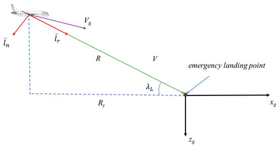
Figure 1.
Diagram of two-dimensional proportional guidance.
By differentiating Equation (1), we obtain
represents the variation in the line-of-sight distance, which corresponds to the change in the magnitude of vector , while denotes the change in the line-of-sight direction, reflecting the variation in the direction of vector within the glide plane. Here, we define , leading to the following equation:
According to the derivative rule for unit vectors in polar coordinates, and are perpendicular, and the magnitude of is 1. Therefore, , and Equation (2) can be expressed as
A two-dimensional line-of-sight coordinate system is formed along the directions of vector and vector . By differentiating Equation (4) again, we obtain:
According to the geometric properties of unit vectors, the derivative of with respect to equals a vector in the opposite direction of , resulting in
Substituting Equation (6) into Equation (5) yields
The projection of the aircraft’s acceleration onto can be expressed as
If the aircraft’s acceleration is defined as perpendicular to the velocity direction, denoted as , and substituted into Equation (8), performing a Laplace transform and simplifying yields
Assuming , we arrive at the following result:
When , the real part of is negative, and the system’s poles are located on the left side of the complex plane. In this case, the system is stable. We can set , which leads to the true PN guidance law:
2.2. Design of 3D Proportional Guidance Law
Three-dimensional proportional navigation is similar to two-dimensional proportional navigation, as it operates on the same fundamental principle: using errors in the line-of-sight (LOS) angular velocity to generate acceleration commands, which are then converted into angular velocity commands to control the actuator surfaces. The key difference in three-dimensional proportional navigation lies in the decomposition of the LOS angular velocity into two components: longitudinal and lateral. As shown in Figure 2, is the unit vector along the LOS direction, the unit vector perpendicular to within the glide plane, and is the vector perpendicular to the glide plane. These vectors form the LOS coordinate system along the directions of , , and .
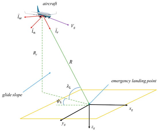
Figure 2.
Diagram of three-dimensional proportional guidance.
After decomposing the LOS angle, two components are obtained: the longitudinal LOS angle and the lateral LOS angle . represents the angle between the UAV-target line and the horizontal plane, while is the angle between the projection of the UAV-target line on the horizontal plane and the x-axis of the ground coordinate system. The range of values for and is . The longitudinal LOS angular velocity is denoted as , and the lateral LOS angular velocity as . Both and can be directly computed by the seeker and transmitted to the flight control system. represents the UAV’s altitude relative to the ground. These LOS angular velocity components generate the longitudinal acceleration command in the direction of and the lateral acceleration command in the direction of , specifically, the following:
Figure 3 illustrates the rotational relationship between the aircraft coordinate system and the line-of-sight (LOS) coordinate system . The LOS coordinate system first rotates by an angle about the axis, followed by a rotation of angle about the current z-axis (which is the axis in the diagram), resulting in alignment with the coordinate system. This leads to the following transformation matrix:
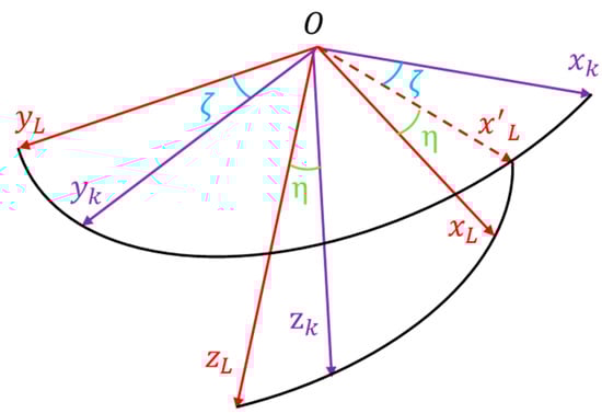
Figure 3.
Transformation relationship between line-of-sight coordinate system and flight path coordinate system.
The angles and can be derived from the geometric relationship between the line-of-sight (LOS) angle and the flight path angle.
where represents the flight path inclination angle, with a range of , and denotes the flight path deviation angle.
Considering the gravitational acceleration g, and transforming and to the flight path coordinate system, we have
The longitudinal and lateral acceleration commands in the flight path coordinate system are obtained as follows:
The roll angle command can be determined using the following equation:
Neglecting the influence of wind, the longitudinal acceleration command in the body-axis coordinate system is given by
For heading control, since we are using the BTT (Bank-to-Turn) control method, we have
Thus, we have obtained the three inputs , , and required for the control law.
3. Control Law
As shown in Figure 4, based on the time-scale separation principle, the control law is divided into inner loops and outer loops. The outer loops for the pitch and yaw channels are designed as acceleration controllers using PI control, while the roll channel’s outer loop is designed for roll angle control using Nonlinear Dynamic Inversion (NDI). The inner loops for all three channels are based on Active Disturbance Rejection Control (ADRC). Since the inner-loop control structures of the three channels are similar, only the inner loop for the pitch channel is discussed in detail here.
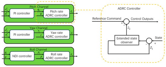
Figure 4.
Controller architecture.
3.1. Outer Loop
- Roll channel;
The outer loop outputs the roll rate command based on the roll angle command, with roll rate control serving as the inner loop for roll angle control. According to the UAV’s rotational dynamics equation about its center of mass, Equation (20) can be derived:
Using the dynamic inversion method, is treated as the desired roll rate, and proportional control is applied for the control of :
In the above equation, represents the roll angle control bandwidth. Substituting Equation (21) into Equation (20) yields the roll angle control law:
where is the roll rate control command generated from the roll angle command, is the roll angle command, and is the current pitch angle.
- 2.
- Pitch channel;
Longitudinal acceleration control uses PI correction in the outer loop, with parameters dynamically adjusted according to dynamic pressure. The longitudinal angular relationship satisfies the following expression:
By differentiating the above equation and considering that the longitudinal acceleration and flight path angle satisfy , combining the two equations gives
Multiplying both sides of the equation by , while neglecting the lateral directional effects, specifically neglecting , results in
where represents the dynamic pressure, is the reference area, is the lift coefficient, and is the mass. Considering and , the transfer function from pitch rate to normal acceleration is obtained as
Since the pitch rate controller can quickly track commands, the relationship between the pitch rate command and the actual pitch rate can be approximated as a first-order inertia system:
where is the control bandwidth of the pitch rate loop. The transfer function from the pitch rate command to the normal acceleration can be expressed as follows:
The above equation has two poles, and , with pole located near the imaginary axis. The control law is designed to cancel pole in order to improve system response. An integrator is introduced to increase the system order and eliminate steady-state error. The design framework of the outer-loop control law for normal acceleration is shown in Figure 5, from which the expression for the pitch rate command can be derived as Equation (29):
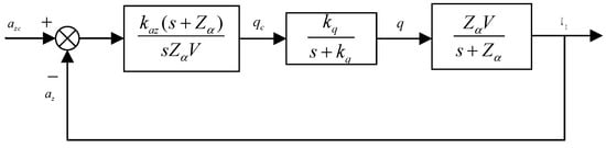
Figure 5.
Diagram of the longitudinal acceleration control.
- 3.
- Yaw channel;
The transfer function from yaw rate to lateral acceleration is given by
where , and with being the lateral force coefficient caused by the sideslip angle.
The relationship between lateral acceleration and sideslip angle can be expressed as
Similar to the longitudinal acceleration control, the angular rate loop can be simplified as a first-order inertia system. By considering the cancellation of pole and introducing an integrator, The design framework of the outer-loop control law for normal acceleration is shown in Figure 6, from which the expression for the yaw rate command can be derived as Equation (32):
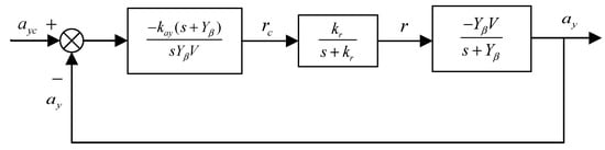
Figure 6.
Diagram of the lateral acceleration control.
3.2. Inner Loop
The pitch rate loop utilizes ADRC control. The control structure is shown in Figure 7:
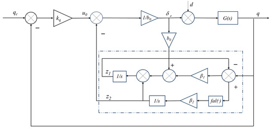
Figure 7.
Inner loop controller architecture for the pitch channel based on ADRC.
The kinematic equation for the pitch angle is
Differentiating both sides of the above equation, we obtain the following:
The angular motion equation about the y-axis can be written as
The general expression for the pitching moment is
Substituting Equation (36) into Equation (35) and simplifying, we obtain
where , is the pitching stability derivative, is the pitching control derivative, is the pitching damping derivative, and is the reference chord length.
Substituting Equation (37) into Equation (34) and simplifying, we obtain
Let and ; then, the Equation (38) can be defined as
Equation (39) can be expressed in the form of a state-space equation as follows:
Design a state observer to monitor the system, and the form of the observer is
where and are the estimations of the angular rate and lumped disturbance for each control channel, respectively; is the measurement value of the angular rate; is the parameter related to the control efficiency; and and are the ESO parameters. The nonlinear function is defined as
where 0 < < 1 and > 0 are the observer parameters, and the sign function is defined as
Reference [23] provides a Lyapunov stability convergence analysis for the ESO, which will not be elaborated upon here. Through proportional control, the closed-loop control bandwidth of the yaw rate controller is , resulting in the final control law output as follows:
4. Hardware-in-the-Loop Simulation
4.1. Hardware-in-the-Loop Simulation Architecture
The hardware-in-the-loop (HIL) simulation system consists of a simulator, flight control system, ground station telemetry software, and data link communication equipment. The UAV’s nonlinear six-degree-of-freedom dynamic model runs on the simulator, while the flight control computer receives model data from the simulator, processes it through the controller, and ultimately sends control command signals back to the simulator to enable model control. The data link facilitates communication both between flight control computers and between the flight control computers and the ground station software. The ground station software includes a display area and a command area, with the display area primarily showing UAV flight status information. The simulator operates on a Speedgoat real-time simulation platform. The ground station computer is responsible for starting the simulator and running the ground station software, establishing communication with the simulator through a network protocol. It connects to a data communication link node to enable wireless communication with all flight control computers involved in the simulation. Communication between the simulator and the flight control computer is conducted via an RS422 serial interface, and the connection between the devices is shown in Figure 8.
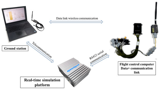
Figure 8.
Device connection diagram for hardware-in-the-loop simulation.
4.2. Hardware-in-the-Loop Simulation Data Analysis
At 0.7 s, the UAV initiated the emergency landing procedure. Prior to this, it maintained level flight at an altitude of 70 m. After receiving the emergency landing command, the UAV entered a dive, with the descent rate gradually increasing. By approximately 16.5 s, the UAV had descended to the final emergency landing altitude of 20 m, with the descent rate reaching −11 m/s. At this point, the emergency landing logic was activated, and the UAV initiated a pull-up maneuver to reduce the descent rate. From the relationship between the flight path angle and the line-of-sight angle in Figure 9c, it is evident that after the emergency landing command was issued, the flight path angle began to converge toward the line-of-sight angle, which aligns with the fundamental characteristics of proportional guidance. Figure 9e shows that the longitudinal line-of-sight angular velocity remained within −1.5°/s, corresponding to the UAV’s descent rate, as reflected in its flight status.
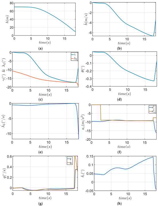
Figure 9.
Hardware-in-the-loop simulation longitudinal data analysis: (a) relative altitude; (b) descent rate; (c) longitudinal line-of-sight angle and flight path angle; (d) pitch angle; (e) longitudinal line-of-sight angular velocity; (f) longitudinal acceleration and longitudinal acceleration command; (g) pitch rate and pitch rate command; (h) elevator deflection command.
After entering the emergency landing phase, the UAV switched to line-of-sight angular velocity guidance. The outer-loop longitudinal control transitioned to a longitudinal acceleration tracking mode, where the longitudinal acceleration command was generated through proportional control based on the longitudinal line-of-sight angular velocity. Figure 9f illustrates that during the approach to the emergency landing point, the changes in longitudinal acceleration closely matched the commanded values, and during the level flight before the emergency landing phase, the longitudinal acceleration remained around −9.8 m/s2. Throughout the descent, the longitudinal acceleration remained relatively stable until the UAV exited the emergency landing logic and performed a pull-up, resulting in a sudden change in longitudinal acceleration. Figure 9g demonstrates that the inner-loop pitch rate command was tracked accurately.
From Figure 10a,b, it can be observed that after entering the emergency landing mode, the lateral acceleration command closely followed the changes in lateral line-of-sight angular velocity. As the UAV approached the target, the lateral line-of-sight angular velocity experienced significant changes, causing the lateral acceleration command to shift toward 0.2 m/s2. The tracking of the lateral acceleration command was accurate, with only small variations, which resulted in the roll angle command remaining near zero. Figure 10e shows the yaw rate command during the emergency landing phase. The yaw rate command was tracked effectively, with the rudder deflection remaining below 2°, ensuring good yaw-rate tracking performance.
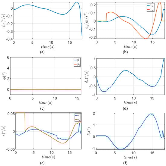
Figure 10.
Hardware-in-the-loop simulation lateral direction data analysis: (a) lateral line-of-sight angular velocity; (b) lateral acceleration and lateral acceleration command; (c) roll angle; (d) aileron deflection command; (e) yaw rate command; (f) rudder deflection command.
5. Flight Test Validation
5.1. Flight Test Mission
Before the flight experiment, a series of tests must be conducted on the UAV. Ground tests include control surface checks, fixed-wing propulsion tests, rotor polarity verification, sensor polarity verification, satellite navigation module testing, and data link range testing for communication reliability. Additionally, a rotor hover test must be performed prior to the UAV’s flight, as shown in Figure 11:
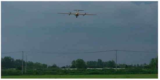
Figure 11.
Compound-wing UAV hover test.
Figure 12 illustrates the mission flight path. In this flight experiment, a rectangular route with seven waypoints was designed, including both a takeoff and landing point. The cruising altitude is set at 70 m relative to the takeoff point, with the path measuring 0.6 km in width and 1.04 km in length, totaling a flight distance of 13 km. Waypoint 1 serves as the rotorcraft takeoff point, where the UAV ascends to 30 m using its rotors before proceeding along the route. The segment between waypoints 1 and 2 marks the transition phase from rotorcraft to fixed-wing mode, during which the altitude remains constant, and the UAV switches to fixed-wing mode before reaching waypoint 2. The section from waypoints 2 to 5 is the climb phase, where the UAV ascends to 70 m relative to the takeoff point by waypoint 5. Upon reaching waypoint 6, the propulsion system is deactivated, and an emergency landing command is issued to simulate an emergency scenario. At this point, the proportional guidance law for emergency landing is automatically engaged, directing the UAV to waypoint 7. As the UAV descends to approximately 20 m above ground under the guidance of the emergency landing law, the vertical landing logic is engaged, with the rotors providing lift for the emergency landing.
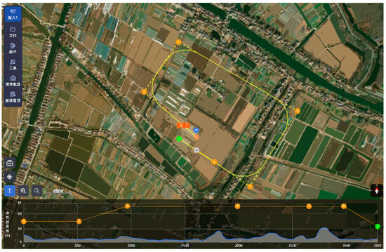
Figure 12.
Flight test mission flight path.
5.2. Flight Test Data Analysis
The flight experiment results were consistent with the hardware-in-the-loop (HIL) simulation. During the flight, the UAV maintained a cruising altitude of 70 m. After receiving the emergency landing command, the UAV began to dive. Comparing the altitude and descent rate data from both the flight experiment and the HIL simulation, it can be observed that the trends are closely aligned. By approximately 15.5 s, the UAV had descended to the final emergency landing altitude of 20 m, with a descent rate of 11.5 m/s. The focus of this experiment was on the relationship between the flight path angle and the line-of-sight angle. Figure 13c shows the curves of the flight path angle and line-of-sight angle obtained from the flight experiment. The curves indicate that after entering the emergency landing mode, the flight path angle gradually converged towards the line-of-sight angle. Throughout the emergency landing, the error between the flight path angle and the line-of-sight angle steadily decreased without any overshoot. In Figure 13e,f, it can be seen that the longitudinal acceleration command, generated from the longitudinal line-of-sight angular velocity, followed the same trend as the line-of-sight angular velocity. Figure 13g shows that in the actual flight, the pitch rate command was accurately tracked. By comparing Figure 9h and Figure 13h, it can be observed that in the actual flight experiment, the elevator deflection required to generate the same pitch rate is greater than that in the simulation. This suggests that the increment in the pitch moment coefficient generated by the elevator in the actual flight is smaller than that predicted by the model.
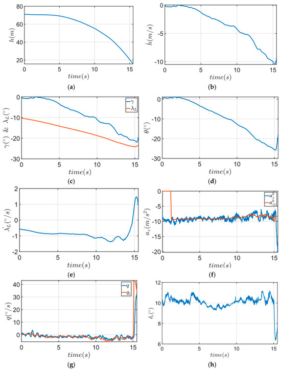
Figure 13.
Flight test longitudinal data analysis: (a) relative altitude; (b) descent rate; (c) longitudinal line-of-sight angle and flight path angle; (d) pitch angle; (e) longitudinal line-of-sight angular velocity; (f) longitudinal acceleration and longitudinal acceleration command; (g) pitch rate and pitch rate command; (h) elevator deflection command.
From Figure 14a,b, it can be seen that during the UAV’s emergency landing phase, the trend of the lateral acceleration command is similar to that of the lateral line-of-sight angular velocity after entering the emergency landing mode. Since the UAV’s velocity is directed toward the landing point during the emergency descent, the lateral line-of-sight angular velocity is zero. However, as the UAV nears the landing point, the lateral line-of-sight angular velocity gradually increases, which is attributed to the seeker losing the lock at close range and requiring re-locking. Figure 14c shows that the roll angle command progressively increases to the right throughout the emergency landing phase. However, the actual lateral acceleration does not change significantly, which can be explained by the presence of strong westerly winds at the test site, causing the UAV to drift to the left. As a result, roll maneuvers were necessary during the emergency landing to counteract the crosswind. Figure 14e demonstrates that the heading inner-loop tracking performed well during the entire process.
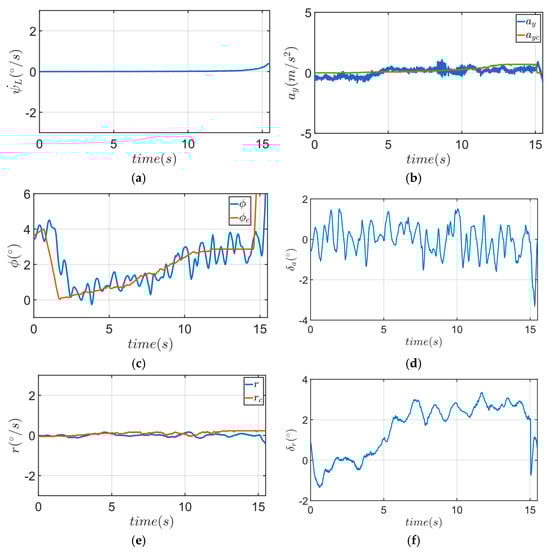
Figure 14.
Flight test lateral direction data analysis: (a) lateral line-of-sight angular velocity; (b) lateral acceleration and lateral acceleration command; (c) roll angle; (d) aileron deflection command; (e) yaw rate command; (f) rudder deflection command.
Figure 15 illustrates the UAV’s mission flight path. The red section of the flight path represents the emergency landing phase, where the UAV executed the emergency descent and approach to the landing point.
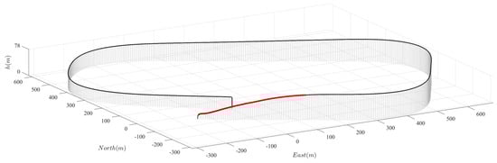
Figure 15.
Flight trajectory of the mission.
6. Conclusions
In summary, emergency landings at low altitudes pose significant challenges to flight safety, particularly in the event of a thrust system failure. As the rise of the low-altitude economy brings increasing attention to the flight safety of small aircraft and UAVs, addressing these challenges has become ever more critical. This paper proposes an emergency landing guidance law based on the principles of three-dimensional proportional guidance, specifically designed for small- and medium-sized compound-wing aircraft. Additionally, the inner-loop control law was designed based on the Active Disturbance Rejection Control (ADRC) theory.
Applying proportional guidance (PG) to UAVs for tracking static emergency landing points eliminates the need to account for tracking errors associated with dynamic targets, as is the case in missile systems. Flight test data demonstrate the algorithm’s remarkable effectiveness. Overall, this study proposes an effective and robust control method that enhances flight safety control during low-altitude emergency landings, allowing for rapid and accurate tracking of the emergency landing point. The findings of this research hold significant practical value for the design and implementation of emergency landing systems for small- and medium-sized aircraft.
Author Contributions
Conceptualization, Z.Z. and Z.G.; methodology, Z.Z.; software, Y.Y. and Z.G.; validation, Z.Z., Z.G. and Y.Y.; formal analysis, Z.Z.; investigation, Y.Y.; resources, Z.Z.; data curation, Y.Y.; writing—original draft preparation, Z.Z. and Y.Y.; writing—review and editing, Z.Z. and Z.G.; visualization, Z.G.; supervision, Y.Y.; project administration, Z.Z. All authors have read and agreed to the published version of the manuscript.
Funding
This research received no external funding.
Data Availability Statement
Data available on request due to restrictions such as privacy or ethical considerations. The data presented in this study are available on request from the corresponding author. The data are not publicly available due to commercial use.
Conflicts of Interest
The company was not involved in the study design, collection, analysis, interpretation of data, the writing of this article or the decision to submit it for publication. The remaining authors declare that the research was conducted in the absence of any commercial or financial relationships that could be construed as a potential conflict of interest.
References
- Coombes, M.; Chen, W.-H.; Render, P. Reachability Analysis of Landing Sites for Forced Landing of a UAS in Wind using Trochoidal Turn Paths. In Proceedings of the 2015 International Conference on Unmanned Aircraft Systems (ICUAS), Denver, CO, USA, 9–12 June 2015. [Google Scholar]
- Coombes, M.; Chen, W.-H.; Render, P. Landing Site Reachability in a Forced Landing of Unmanned Aircraft in Wind. J. Aircr. 2017, 54, 1219–1234. [Google Scholar] [CrossRef]
- Fitzgerald, D.; Walker, R.; Campbell, D. A Vision Based Emergency Forced Landing System for an Autonomous UAV. In Proceedings of the Eleventh Australian International Aerospace Congress, Melbourne, Australia, 17 March 2005. [Google Scholar]
- Izuta, S.; Takahashi, M. Path Planning to Improve Reachability in a Forced Landing. J. Intell. Robot. Syst. 2017, 86, 291–307. [Google Scholar] [CrossRef]
- Fang, X.; Jiang, J.; Chen, W.H. Model Predictive Control With Wind Preview for Aircraft Forced Landing. IEEE Trans. Aerosp. Electron. Syst. 2023, 59, 3995–4004. [Google Scholar] [CrossRef]
- Chen, Y.; Wang, J.; Wang, C.; Shan, J.; Xin, M. A modified cooperative proportional navigation guidance law. J. Frankl. Inst. 2019, 356, 5692–5705. [Google Scholar] [CrossRef]
- Shin, H.S.; Li, K.B. An Improvement in Three-Dimensional Pure Proportional Navigation Guidance. IEEE Trans. Aerosp. Electron. Syst. 2021, 57, 3004–3014. [Google Scholar] [CrossRef]
- Ghosh, S.; Ghose, D.; Raha, S. Capturability of Augmented Pure Proportional Navigation Guidance Against Time-Varying Target Maneuvers. J. Guid. Control Dyn. 2014, 37, 1446–1458. [Google Scholar] [CrossRef]
- Jeon, I.-S.; Lee, J.-I.; Tahk, M.-J. Impact-Time-Control Guidance with Generalized Proportional Navigation Based on Nonlinear Formulation. J. Guid. Control Dyn. 2016, 39, 1885–1890. [Google Scholar] [CrossRef]
- Ghose, D. On the Generalization of True Proportional Navigation. IEEE Trans. Aerosp. Electron. Syst. 1994, 30, 545–555. [Google Scholar] [CrossRef]
- Prasanna, H.M.; Ghose, D. Retro-Proportional-Navigation: A New Guidance Law for Interception of High-Speed Targets. J. Guid. Control Dyn. 2012, 35, 377–386. [Google Scholar] [CrossRef]
- Ulybyshev, Y. Terminal Guidance Law Based on Proportional Navigation. J. Guid. Control Dyn. 2005, 28, 821–882. [Google Scholar] [CrossRef]
- Weiss, H.; Rusnak, I.; Hexner, G. Adaptive Proportional Navigation Guidance. In Proceedings of the 58th Israel Annual Conference, Aviv & Haifa, Israel, 14–15 March 2018. [Google Scholar]
- Adler, F.P. Missile Guidance by Three-Dimensional Proportional Navigation. J. Appl. Phys. 1956, 27, 500–507. [Google Scholar] [CrossRef]
- Becker, K. Closed-Form Solution of Pure Proportional Navigation. IEEE Trans. Aerosp. Electron. Syst. 1990, 26, 526–533. [Google Scholar] [CrossRef]
- Yang, C.D.; Yang, C.C. Optimal Pure Proportional Navigation for Maneuvering Targets. IEEE Trans. Aerosp. Electron. Syst. 1997, 33, 949–957. [Google Scholar] [CrossRef]
- Yuan, P.J.; Chern, J.S. Solutions of True Proportional Navigation for Maneuvering and Nonmaneuvering Targets. J. Guid. Control Dyn. 1992, 15, 268–271. [Google Scholar] [CrossRef]
- Yang, C.D.; Yang, C.C. Analytical Solution of 3D True Proportional Navigation. IEEE Trans. Aerosp. Electron. Syst. 1996, 32, 1509–1522. [Google Scholar] [CrossRef]
- Yang, C.D.; Yang, C.C. A Unified Approach to Proportional Navigation. IEEE Trans. Aerosp. Electron. Syst. 1997, 33, 557–567. [Google Scholar] [CrossRef]
- Ratnoo, A. Analysis of Two-Stage Proportional Navigation with Heading Constraints. J. Guid. Control Dyn. 2016, 39, 156–164. [Google Scholar] [CrossRef]
- Guelman, M. The Closed-Form Solution of True Proportional Navigation. IEEE Trans. Aerosp. Electron. Syst. 1976, 12, 472–482. [Google Scholar] [CrossRef]
- Guo, B.Z.; Zhao, Z. On the convergence of an extended state observer for nonlinear systems with uncertainty. Syst. Control Lett. 2011, 60, 420–430. [Google Scholar] [CrossRef]
- Eng, P. Path planning, guidance and control for a UAV forced landing. Doctoral dissertation, Queensland University of Technology, Brisbane, Queensland, Australia, 2011. [Google Scholar]
Disclaimer/Publisher’s Note: The statements, opinions and data contained in all publications are solely those of the individual author(s) and contributor(s) and not of MDPI and/or the editor(s). MDPI and/or the editor(s) disclaim responsibility for any injury to people or property resulting from any ideas, methods, instructions or products referred to in the content. |
© 2024 by the authors. Licensee MDPI, Basel, Switzerland. This article is an open access article distributed under the terms and conditions of the Creative Commons Attribution (CC BY) license (https://creativecommons.org/licenses/by/4.0/).