Abstract
In fields such as manufacturing and aerospace, remaining useful life (RUL) prediction estimates the failure time of high-value assets like industrial equipment and aircraft engines by analyzing time series data collected from various sensors, enabling more effective predictive maintenance. However, significant temporal diversity and operational complexity during equipment operation make it difficult for traditional single-scale, single-dimensional feature extraction methods to effectively capture complex temporal dependencies and multi-dimensional feature interactions. To address this issue, we propose a Dual-Path Interaction Network, integrating the Multiscale Temporal-Feature Convolution Fusion Module (MTF-CFM) and the Dynamic Weight Adaptation Module (DWAM). This approach adaptively extracts information across different temporal and feature scales, enabling effective interaction of multi-dimensional information. Using the Commercial Modular Aero-Propulsion System Simulation (C-MAPSS) dataset for comprehensive performance evaluation, our method achieved RMSE values of 0.0969, 0.1316, 0.086, and 0.1148; MAPE values of 9.72%, 14.51%, 8.04%, and 11.27%; and Score results of 59.93, 209.39, 67.56, and 215.35 across four different data categories. Furthermore, the MTF-CFM module demonstrated an average improvement of 7.12%, 10.62%, and 7.21% in RMSE, MAPE, and Score across multiple baseline models. These results validate the effectiveness and potential of the proposed model in improving the accuracy and robustness of RUL prediction.
1. Introduction
In today’s large-scale production environments, equipment often operates under high-load conditions, which accelerates the wear and tear of critical components, significantly increasing the risk of equipment failure and leading to severe economic losses and unplanned downtime. Traditional maintenance strategies, such as corrective maintenance, time-based maintenance, and condition-based maintenance, are no longer sufficient to meet the demands of modern, efficient operations [1]. As a key technology in Prognostics and Health Management (PHM), remaining useful life (RUL) prediction plays a crucial role in providing timely and accurate assessments of equipment degradation, offering valuable insights for predictive maintenance. However, the complexity of modern industrial systems, particularly in the context of temporal variability and operational complexity, results in progressive or sudden changes in equipment conditions over time, leading to significant differences in system states at various points. Moreover, under diverse operating conditions, the equipment’s state and RUL are greatly affected, and the interaction between different feature dimensions becomes highly complex [2]. These challenges highlight the need for advanced predictive methods that can better capture the intricate interactions between temporal features and the long-term and short-term dependencies critical for accurate RUL prediction.
Currently, remaining useful life prediction methods can be categorized into three main types: physics-based models, data-driven models, and hybrid models. Physics-based models rely on understanding the failure mechanisms of equipment, analyzing its degradation from fundamental principles, failure mechanisms, and key components. However, as equipment becomes increasingly complex, the construction of physics-based models necessitates fitting a large number of parameters, making model building overly challenging [3]. Hybrid models integrate the strengths of both physics-based and data-driven approaches, improving the accuracy of RUL prediction. Nevertheless, due to their inherent complexity, their application in real-world engineering is limited. In contrast, data-driven models, which leverage technologies such as big data and the Internet of Things (IoT), automatically extract deep features from vast historical datasets, significantly reducing the need for domain expertise and showing broader application prospects [4].
Data-driven RUL prediction methods can be broadly classified into two categories: statistical learning-based methods and machine learning-based methods. Statistical methods aim to model the degradation process of equipment by constructing statistical models to simulate the probability distribution of equipment failure. Machine learning-based approaches focus on extracting useful degradation information from historical monitoring data to address the RUL prediction as a regression problem. However, traditional machine learning methods heavily rely on domain expertise for feature engineering. With the development of deep learning technologies, an increasing number of studies have shifted toward deep learning, which can automatically extract deep features from data, reducing the dependence on manual feature engineering. Therefore, this paper will focus on exploring and analyzing the application of deep learning methods in RUL prediction [5].
With the advancement of sensor deployment and computing power, deep learning has enabled neural networks to automatically extract deeper features from historical data, resulting in more accurate remaining useful life predictions. Currently, the more widely used models are Recurrent Neural Networks (RNNs) and Convolutional Neural Networks (CNNs). RNNs excel at capturing temporal features, while CNNs are effective at extracting multi-scale features [6]. For example, RNNs are often employed to capture regression features in time series data. Khandelwal et al. proposed an RNN-based model for predicting the remaining useful life of lithium-ion batteries by analyzing battery degradation under various operating conditions [7]. Sayah et al. proposed a robustness testing framework for deep LSTM models in RUL prediction, analyzing the model’s resilience and performance under stress functions, and validated it using the C-MAPSS dataset [8]. However, since the input of each time step in an RNN depends on the output of the previous time step, there is a risk of information loss, and the vanishing gradient problem can occur when processing long sequences. In contrast, CNNs can process data in parallel, avoiding the information loss and vanishing gradient issues that arise in RNNs due to sequential processing. When handling time series data, CNNs often employ sliding time windows and perform convolution operations along the temporal dimension to capture the mapping relationships between each time window and the RUL labels. For instance, Keshun et al. proposed a 3D attention-enhanced hybrid neural network model based on CNN and BiLSTM, which extracts local features through a convolutional network and leverages the BiLSTM framework to learn long-dependency nonlinear features, while incorporating a 3D attention module to enhance the model’s learning capability and interpretability [9]. Additionally, in recent years, Multilayer Perceptrons (MLPs) have shown great potential in time series prediction. With their strong representation learning capabilities, MLPs can effectively capture complex temporal dependencies and patterns. For instance, The MLP-Mixer architecture proposed by Tolstikhin et al., although originally designed for image processing, has proven effective for RUL prediction by mixing local features at each time step and global features across time steps. This approach captures temporal degradation information without relying on convolutions or attention mechanisms, offering a new way to process time series data [10]. Although these studies have improved model accuracy in RUL prediction, certain limitations remain.
Firstly, many of these methods focus primarily on feature extraction along the temporal dimension, while neglecting the diversity of features in other dimensions. For example, Zhang et al. proposed a multi-head dual sparse self-attention network, which introduced ProbSparse and LoSparse strategies to optimize the efficiency of time series processing and reduce computational complexity [11]. Zhang et al. developed a novel bidirectional gated recurrent unit with a temporal self-attention mechanism (BiGRU-TSAM) that assigns self-learned weights to RUL prediction tasks at different time points, improving the model’s ability to capture temporal dependencies [12]. Li et al. introduced an RUL prediction method that combines domain knowledge with gated recurrent units (GRUs) and a dual attention mechanism, using temporal attention along with domain knowledge to enhance both accuracy and interpretability [13]. Chen et al. utilized convolutional neural networks to extract temporal features and combined them with a Bayesian long short-term memory network (B-LSTM) to construct a multivariate time series prediction model [14]. Ekambaram et al. introduced a lightweight multilayer perceptron architecture called TSMixer, showcasing the potential of MLP in time series prediction, though it lacks effective interaction across different feature scales [15]. Zhao et al. combined GRU with a multi-head attention mechanism to encode temporal features from battery capacity time series data, while using a re-zero MLP-Mixer model to extract higher-level features, enhancing RUL prediction accuracy for lithium-ion batteries [16]. Jiang et al. proposed a dual-attention-based multiscale convolutional neural network (DAMCNN) that utilizes precise time stage division and multiscale temporal feature extraction to efficiently predict the remaining useful life of rolling bearings [17]. Wang et al. proposed a hybrid model combining Bi-LSTM, Temporal Convolutional Networks (TCNs), and an attention mechanism, which captures time series features at different levels and enhances the ability to handle dynamic degradation in complex systems [18]. Mao et al. proposed a method combining Multi-Scale Convolutional Neural Networks (MCNNs), Decomposition Linear Layer, and Conformal Quantile Regression (CQR), which improves the accuracy of RUL predictions by capturing both long-term trends and local variations in time series features [19]. Lei et al. proposed an interpretable operational condition-aware attention-based domain adaptive network, which aligns the temporal features of the source and target domains through a domain adaptation method and eliminates the impact between time-varying operating conditions and monitoring data via an Operational Condition Attention (OCA) subnetwork, thereby improving the model’s predictive accuracy under complex conditions [20]. Wang et al. proposed a prediction model based on the self-attention mechanism and Temporal Convolutional Network, which captures temporal dependencies through TCN and adaptively assigns weights to time features using the self-attention mechanism, improving the accuracy of remaining useful life predictions [21]. Ren et al. proposed a continuous learning framework based on kernel-space gradient projection, which uses a multi-kernel group convolution module to combine convolution operations at different scales, automatically capturing degradation features over time and adaptively adjusting attention allocation based on operational condition information [22]. Although these methods have made significant progress in temporal feature extraction, they fail to adequately consider critical information from the feature dimension, potentially leading to the loss of key global information and feature interrelationships, which could negatively impact RUL prediction performance under complex working conditions.
Secondly, many of these studies focus on local feature extraction and specific scales, lacking in-depth exploration of cross-scale feature correlations. For instance, Zhang et al. proposed a parallel hybrid neural network combining 1D convolutional neural networks (1-DCNNs) and bidirectional gated recurrent units (BiGRUs) to simultaneously extract both temporal and feature dimension information from historical data for RUL prediction [23]. Remadna et al. introduced a hybrid deep learning model that combines CNN and bidirectional long short-term memory networks, extracting features across both the temporal and feature dimensions to enhance RUL prediction performance [24]. En et al. proposed a dual-mixer model based on supervised contrastive learning, which progressively integrates temporal and feature dimensions while maintaining the consistency of relationships between sample features and degradation processes through a training method called Feature Space Global Relationship Invariance (FSGRI) [25]. Zhang et al. proposed a Self-Attention Mechanism Network with Spatio-Temporal Feature Extraction (SAMN-STFE), which utilizes Convolutional Neural Networks and Bidirectional Long Short-Term Memory networks to extract spatial and temporal features [26]. Deng et al. proposed a remaining useful life prediction method for aero engines based on a CNN-LSTM-Attention framework, where local features are extracted using CNN and then combined with LSTM and an attention mechanism for RUL prediction [27]. While these methods improve performance in processing time series data, they lack a flexible weight allocation mechanism during feature fusion, making it difficult to effectively adjust the model’s focus when dealing with different types of degradation information, leading to suboptimal results.
Inspired by the MLP-Mixer architecture, this paper proposes a Dual-Path Interaction Network model to address the aforementioned issues. The model captures complex relationships between the temporal and feature dimensions through a dual-path structure, enhancing information interaction during feature extraction, thereby improving the quality of feature representation and the accuracy of predictions. This approach effectively avoids the limitations of single-path structures, which may overlook critical features. However, despite the dual-path structure’s ability to capture both temporal and feature dimension information, the feature extraction process still focuses mainly on local and specific scales, failing to fully cover cross-scale information correlations. To further enhance the comprehensiveness and richness of feature extraction, this paper designs a Multiscale Temporal-Feature Convolution Fusion Module (MTF-CFM). This module introduces multiple convolution kernels of different scales through a 1D Convolutional Neural Network for multiscale feature extraction, and generates more expressive feature representations for both the temporal and feature dimensions through concatenation and splitting operations. The multiscale convolution kernel design enables more comprehensive capture of information across different temporal and feature scales. Nevertheless, the effectiveness of feature interaction and fusion largely depends on the proper allocation and dynamic adjustment of weights. To address this, the paper further introduces a Dynamic Weight Adaptation Module (DWAM), which enables dynamic interaction and adaptive weight adjustments between the temporal and feature dimensions, enhancing the model’s predictive performance and flexibility. As a result, the proposed model significantly improves RUL prediction accuracy.
The contributions of this paper are as follows:
- Proposing the Dual-Path Interaction Network architecture: This paper introduces a novel dual-path interaction network architecture, which utilizes a dual-path structure to capture the complex relationships between the temporal and feature dimensions. By preserving more information interactions during the feature extraction process, the dual-path structure improves the quality of feature representations and the accuracy of predictions, effectively avoiding the issue of single-path models neglecting critical features.
- Designing the Multiscale Temporal-Feature Convolution Fusion Module (MTF-CFM): To further enhance the comprehensiveness and richness of feature extraction, this paper designs the MTF-CFM module. By introducing multiple convolutional kernels of different scales for multiscale feature extraction, combined with operations such as concatenation and splitting, the module captures features across both temporal and feature dimensions, generating feature representations with richer expressive capabilities.
- Introducing the Dynamic Weight Adaptation Module (DWAM): To address the challenges of weight allocation and dynamic adjustment in feature interaction and fusion, this paper introduces the Dynamic Weight Adaptation Module. This module enables dynamic interaction and adaptive weight adjustment between the temporal and feature dimensions, improving the model’s prediction performance and flexibility, thereby enhancing the accuracy of RUL prediction.
- Experimental validation on the C-MAPSS dataset: Comprehensive comparative and ablation experiments were conducted on the C-MAPSS dataset to systematically validate the effectiveness and superiority of the proposed method. The results show that the proposed approach significantly outperforms existing methods in terms of RMSE and other evaluation metrics, highlighting its practical applicability. In particular, independent experiments on the MTF-CFM module demonstrated its wide applicability and substantial improvements in model performance across various network architectures, further underscoring its versatility and generalization capability.
2. Materials and Methods
2.1. Remaining Useful Life
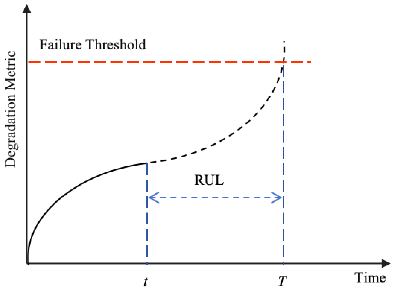
Remaining useful life is defined as the time duration from the current moment until the end of the equipment’s operational life, that is, the time remaining until the system reaches its failure threshold [28]. By analyzing equipment condition monitoring data, environmental data, and other historical information, RUL helps assess the degradation state and predict the failure time of the equipment, providing critical insights for formulating maintenance strategies. RUL is expressed as follows:
where T denotes the moment when the device is no longer performing a function, t denotes the current moment, and denotes the current health state data. A schematic diagram of the device RUL is shown in Figure 1.
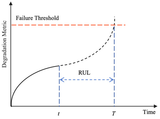
Figure 1.
Equipment RUL schematic.
2.2. Methodologies
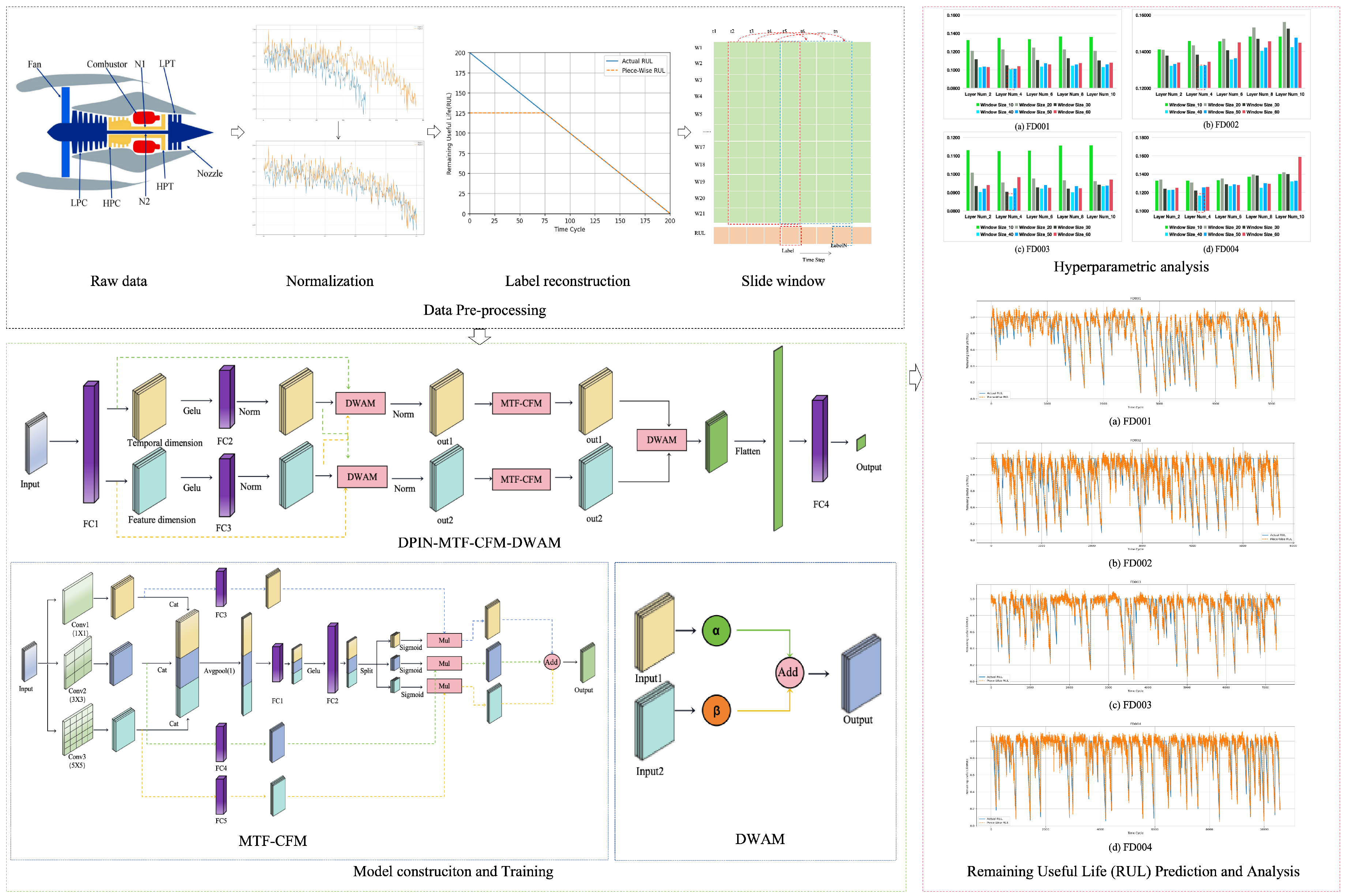
Building on the previous work, we propose a method for RUL prediction called the Dual-Path Interaction Network for RUL Prediction (DPIN-RUL). The overall framework of the model is illustrated in Figure 2. DPIN-RUL consists of three main components: the Dual-Path Interaction Network (DPIN), the Multiscale Temporal-Feature Convolution Fusion Module, and the Dynamic Weight Adaptation Module. The Dual-Path Interaction Network (Section 2.2.1) is responsible for feature extraction and interaction, MTF-CFM (Section 2.2.2) captures and integrates multiscale spatiotemporal information, and DWAM (Section 2.2.3) dynamically adjusts the weights to enhance the accuracy of RUL prediction.
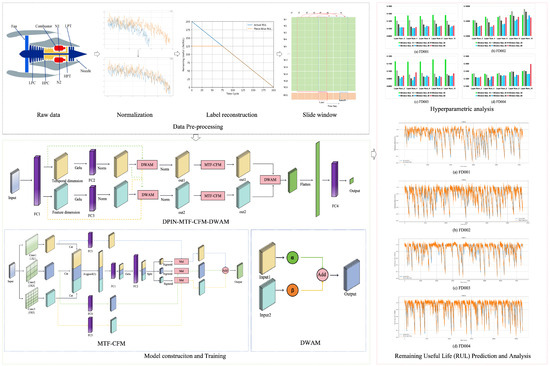
Figure 2.
The general architecture of the proposed model.
2.2.1. Dual-Path Interaction Network
Inspired by the MLP-Mixer framework, this paper proposes a Dual-Path Interaction architecture for RUL prediction. This architecture sets up two parallel paths to extract features independently along the temporal and feature dimensions, effectively capturing complex relationships between these dimensions. The dual-path structure not only ensures the retention of more information interactions but also allows each path to focus on processing features from a single dimension, enabling better feature separation and extraction. This enhances the quality of feature representations and improves the accuracy of RUL predictions. Finally, the outputs from both paths are fused, and a linear layer is applied to generate precise RUL prediction results.
As shown in Figure 3, the input generates two identical outputs after passing through the fully connected layer with shared parameters.

Figure 3.
Dual-Path Interaction Network.
In this context, the refers to the input data, while W and b represent the weight matrix and bias vector of the fully connected layer , respectively. These parameters are used to modify the outputs and , adjusting the network’s learned representation.
- Time and Feature dimension information extraction:Initially, the model applies the activation function to input features and , introducing non-linear transformations (as depicted by the layer in the figure). This step enables the model to capture intricate patterns and non-linear relationships within the input data, facilitating the extraction of complex dependencies across both temporal and feature dimensions. Subsequently, the transformed features are passed through fully connected layers and , where linear transformations are performed via learnable weights and biases, aimed at reconstructing the spatial representations of the temporal and feature dimensions. Next, layer normalization (denoted as in the figure) is applied to the feature representations along the temporal and feature axes, ensuring consistency by mitigating differences in feature scales, which stabilizes the training process and promotes smoother gradients and convergence. Finally, the model produces the outputs and , representing the extracted information from the temporal and feature dimensions, respectively. By leveraging this extraction mechanism, the model enhances its robustness and generalization capabilities when dealing with complex temporal features, thereby improving its performance across diverse application scenarios. The process is as follows.In this process, input needs to be transposed to adjust its shape for temporal feature extraction, while the activation function is applied to introduce non-linearity. and represent the weight matrix and bias vector of the fully connected layer , and and correspond to those of the fully connected layer . These matrices and vectors are primarily used to perform computations on the input, generating new linear combinations. is then applied to these combinations to normalize the outputs and , ensuring they have a mean of 0 and a variance of 1.
- Interaction between Temporal and Feature Dimension Information:Taking the temporal dimension as an example, the output feature captures the complex temporal dependencies inherent in the input data, while , though primarily handling feature dimension information, still retains a degree of temporal correlation. To generate the final temporal dimension output , we perform element-wise summation of the original input feature , the processed temporal feature , and the feature dimension output (denoted by the operation in the figure), effectively fusing the features. The result of this fusion is then passed through a layer normalization process (represented as in the figure) to produce the representative temporal dimension output , thereby enhancing the model’s robustness and generalization ability. The processing of feature dimension information follows a similar approach. Although primarily captures temporal dimension features, it still contains some information from the feature dimension. By fusing these elements, the representation of the feature dimension is strengthened. The element-wise summation of the original input feature , the processed feature dimension output , and the temporal dimension feature (illustrated by the operation) is followed by layer normalization to obtain a stable feature dimension output .Either or needs to be transposed to ensure that , , , and have the same shape. Then, element-wise summation is performed across different dimensions (temporal and feature dimensions, as shown by the operation in Figure 3), followed by applying (as indicated by the operation in Figure 3) for layer normalization.
- Multi-layer Feature Extraction and Fusion Mechanism:We introduce the Dual-Path Interaction Layer (DPI Layer), a mechanism akin to the mixing layers in MLP-Mixer [10], for deep feature extraction and fusion through the stacking of multiple DPI layers. Compared to a single feature extraction layer, which has inherent limitations in capturing complex patterns, the multi-layer DPI structure allows for iterative feature extraction and interaction, enabling the model to capture more intricate and in-depth information across both temporal and feature dimensions. Within each DPI layer, the model undergoes multiple rounds of non-linear transformations and normalization, which enhances its robustness and generalization capability. By stacking multiple DPI layers, the model progressively extracts richer multidimensional features, leading to a significant improvement in the accuracy of remaining useful life prediction. After several iterations of processing the temporal and feature dimensions, the final outputs from both dimensions, and , are fused through element-wise summation to obtain a more comprehensive feature representation . Finally, the fused feature is flattened and passed through a fully connected layer for a linear transformation, generating the final RUL prediction output.Element-wise summation is performed between and (as shown by the operation in the Figure 3). The Flatten operation unfolds the data, and W and b represent the weight matrix and bias vector of the fully connected layer . is the final output, which represents the RUL prediction for each sample.
2.2.2. Multiscale Temporal-Feature Convolution Fusion Module (MTF-CFM)
In the previous section, we utilized N Dual-Path Interaction layers to extract temporal dimension features and feature dimension features . However, there remain certain limitations in terms of feature richness and multi-scale feature capturing. While N DPI layers are capable of extracting temporal and feature information, this extraction is largely confined to local features and specific scales, failing to comprehensively capture multi-scale features. Moreover, a single feature extraction path may overlook critical multi-scale features, limiting the model’s ability to fully understand and represent complex data patterns. To address these issues, this paper introduces the Multi-scale Temporal-Spatial Feature Convolutional Fusion Module, which employs convolutional kernels of varying sizes to extract multi-scale features from the input data. By combining connection and splitting operations, this module generates feature representations with enriched expressiveness across both temporal and feature dimensions.
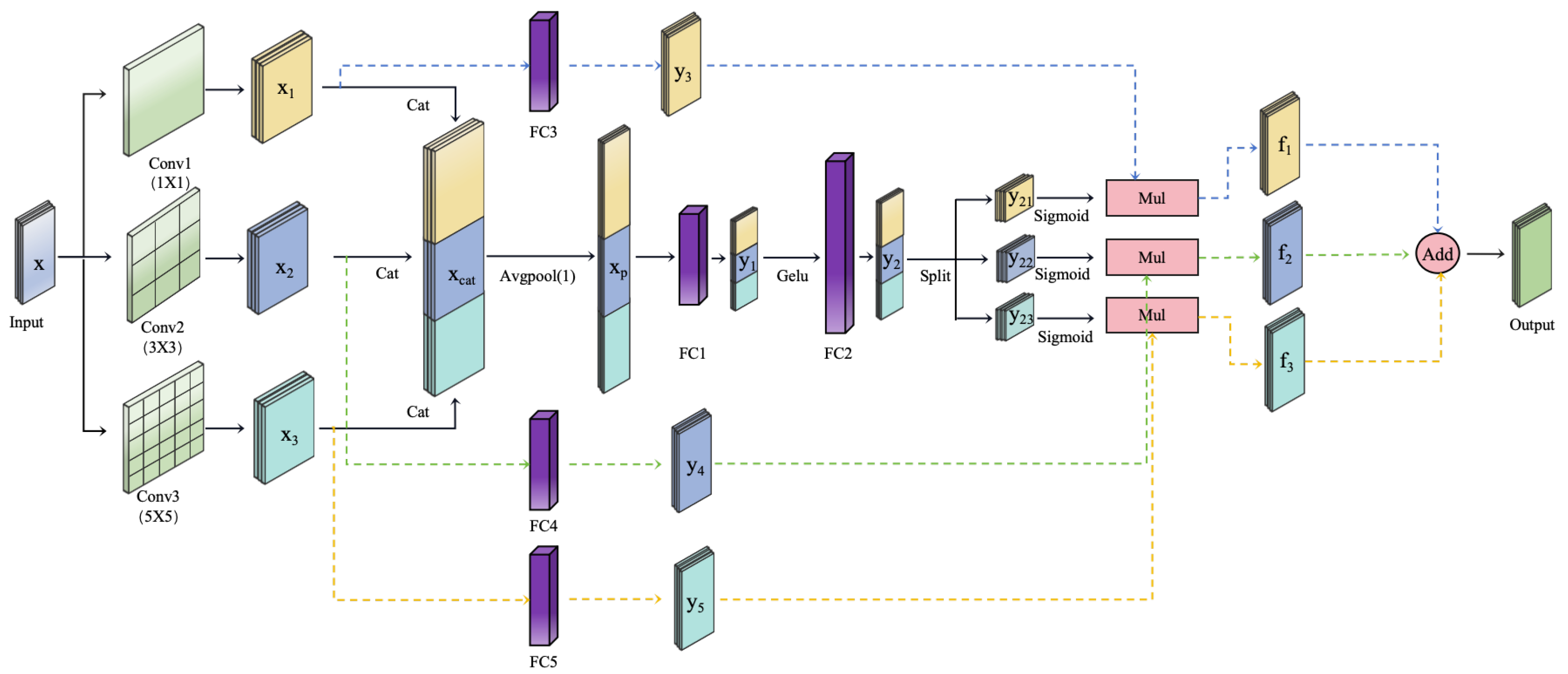
As shown in Figure 4, taking the temporal dimension features as an example, the MTF-CFM module enhances the model’s ability to extract both local and global information from temporal features through parallel 1D convolution layers of varying kernel sizes: 1 × 1 ( in the figure), 3 × 3 (), and 5 × 5 (). The 1 × 1 convolution provides the smallest receptive field, capturing features point-wise and efficiently fusing channel information, thus focusing on local details and point-specific features. The 3 × 3 convolution, with a moderate receptive field, captures shorter temporal dependencies in local regions, extracting medium-scale local features. The 5 × 5 convolution, offering a larger receptive field, spans a longer temporal range, allowing the model to capture global patterns and long-range dependencies. By employing this parallel multi-scale convolution operation, the model is capable of comprehensive feature extraction from temporal data across different receptive fields, ensuring enriched information representation at local, medium, and global levels.
where x represents the input, and refers to convolution, with the weights and biases corresponding to the 1D convolutional layers for different kernel sizes. Specifically, i = 1, 2, 3 correspond to the 1 × 1, 3 × 3, and 5 × 5 convolutions, respectively.
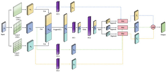
Figure 4.
Multiscale Temporal-Feature Convolution Fusion Module.
Furthermore, the outputs of the three convolutional layers with different scales are integrated through a concatenation operation (denoted as the cat operation in the figure). The output features , , and , derived from the 1 × 1, 3 × 3, and 5 × 5 convolution kernels, are concatenated along the feature channel dimension to form a comprehensive multi-scale feature representation . This integration ensures that the model simultaneously focuses on both local details and global patterns. To further optimize the representation of the feature dimension, an average pooling operation (denoted as in the figure) is applied, reducing the feature dimension to a single dimension and removing redundant feature information. This approach retains only the temporal dimension features, thereby improving the efficiency of feature processing by concentrating on the temporal aspect.
where represents the concatenation operation, which combines , , and along the feature dimension. refers to an adaptive average pooling operation, which adjusts the output size to the desired target dimension, in this case, reducing the feature dimension of to 1.
Subsequently, the multi-scale integrated feature is split (denoted as the split operation in the figure) into the corresponding outputs of the 1 × 1, 3 × 3, and 5 × 5 convolution kernels, , , and , and a activation function is applied to generate feature weights. These weights are used to dynamically adjust the importance of features at each scale. Simultaneously, the original convolution outputs , , and are passed through fully connected layers , and , respectively, for linear transformation, resulting in feature vectors , , and . The generated weights are then applied element-wise to the corresponding feature vectors , and (represented by the operation in the figure), yielding the weighted features , , and . Finally, , , and are summed element-wise (denoted as the operation) to produce the final output feature that encapsulates multi-scale temporal information.
where and through and correspond to the weight matrices and biases of fully connected layers to , respectively. refers to the Gaussian Error Linear Unit activation function. (as shown by the operation) represents the operation that divides into , , and . refers to the activation function that generates feature weights , , and , which are multiplied by the corresponding vectors (represented by the operation) to obtain the weighted features. Finally, the three branches of weighted features are summed element-wise (as denoted by the operation) to produce the final output.
This dynamic weighting and fusion mechanism allows for the full expression and integration of features across different convolutional scales, enhancing the model’s capacity to capture multi-scale temporal dependencies and global patterns. The combination of concatenation and splitting operations ensures that information extracted from different convolution kernels is effectively fused, while the splitting process allows the model to extract richer contextual information from the extended temporal dimension features. This improves the model’s ability to process and accurately represent temporal features, ensuring it can flexibly handle both local and global patterns in time series data.
2.2.3. Dynamic Weight Adaptation Module (DWAM)
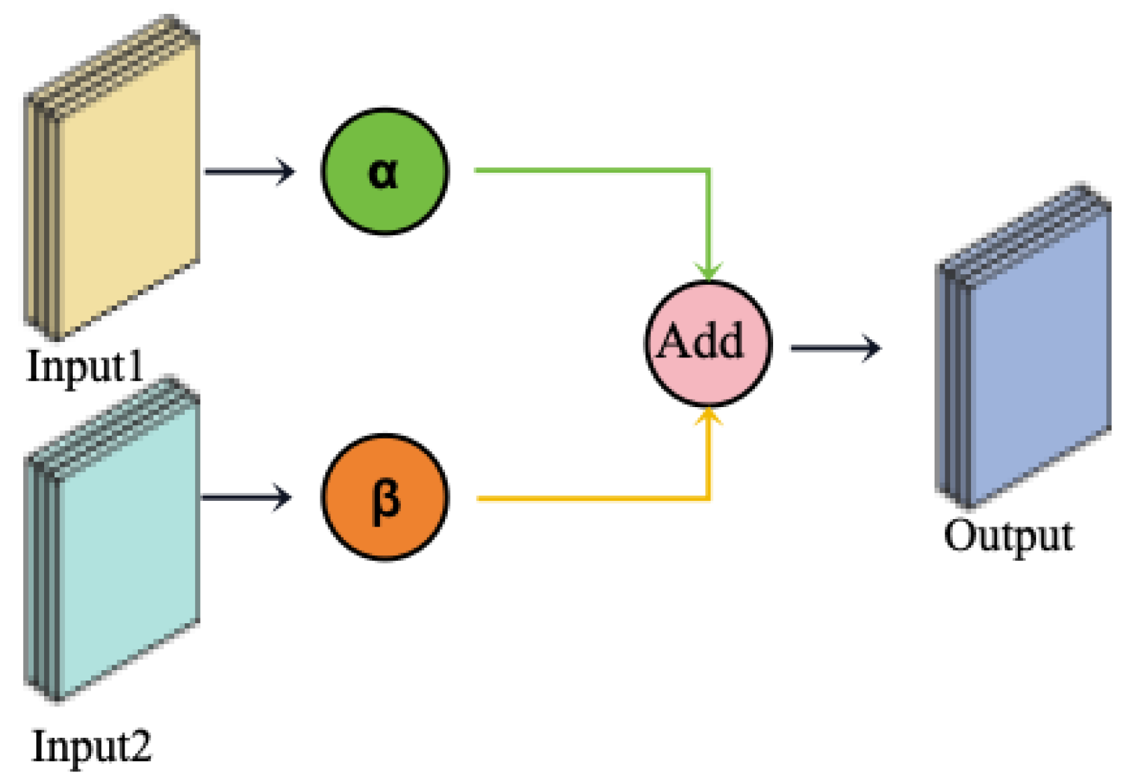
In the previous work, multi-scale temporal and feature dimension features were extracted, and these features were weighted and fused. However, the effectiveness of feature interaction and fusion largely depends on the reasonable allocation and dynamic adjustment of feature weights. To address this issue, this paper introduces the Dynamic Weight Adaptation Module, which aims to achieve dynamic weight adjustment during feature fusion. This optimizes feature interaction and improves the model’s predictive performance and flexibility. The core of DWAM lies in the introduction of dynamic weights, which flexibly adjust the contribution of each feature during the final fusion based on the importance of different features. The DWAM model is shown in Figure 5.
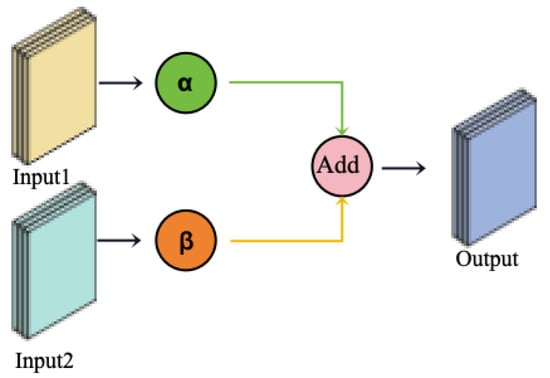
Figure 5.
Dynamic Weight Adaptation Module.
In the model architecture described in this paper, DWAM sets dynamic weight variables to perform dynamic weighted fusion on temporal features ( and ) and feature dimension features ( and ). Taking temporal feature fusion as an example, DWAM calculates a comprehensive feature representation based on the dynamic weights of the input (output from temporal feature extraction) and (output from feature dimension extraction), as shown in the following equation:
where and are dynamic weight variables which can be adjusted according to the importance of the features, ensuring a reasonable contribution of the temporal and feature dimensions in the comprehensive feature representation. In the final output, the temporal information and feature information incorporate the dynamic weight sum, leading to the overall model output:
By adaptively adjusting the dynamic weights, DWAM effectively enhances the model’s flexibility and robustness, allowing for more reasonable weight allocation between different features, thereby improving the accuracy of RUL prediction.
3. Experiment
In this section, we focus on the C-MAPSS dataset, which is very widely used in the field of RUL, to compare with other methods. Section 3.1 presents information about this dataset, Section 3.2 performs preprocessing work on the dataset, Section 3.3 performs hyperparametric simulation experiments, Section 3.4 performs controlled experiments to verify the validity of the model, and Section 3.5 performs ablation experiments to verify the validity of the module.
In addition, all experiments conducted in this paper were carried out in an experimental platform with PyTorch2.2.2, Python3.9.19, installed with NVIDIA GeForce RTX4080. And in order to avoid generating randomness, all experiments were replicated five times and averaged.
3.1. Dataset Description
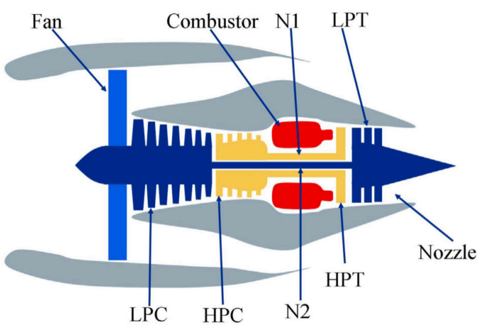
This paper focuses on experiments in the C-MAPSS dataset, which is very widely used in the PHM field, and is a simulated engine degradation dataset developed and made available by NASA, specifically for health management studies of aero engines.
Figure 6 shows the architecture of the aircraft engine, with specific parameters detailed in Table 1. Besides Table 2 provides detailed information on the data collected by the deployed sensors.

Figure 6.
Schematic diagram of the engine model in the C-MAPSS dataset.

Table 1.
Engine Model Structure Variables in the C-MAPSS Dataset.

Table 2.
Description of schematic diagram of the engine model.
The C-MAPSS dataset consists of four different sub-datasets: FD001, FD002, FD003, and FD004. Each sub-dataset contains multiple instances of engine degradation, and for each instance, there are several time steps of data recorded before the occurrence of a failure. Each time step’s record includes various sensor measurements and operational conditions. The dataset description is shown in Table 3.

Table 3.
Description of C-MAPSS dataset.
In addition, since the RUL prediction problem of the engine can be applied to the regression problem, for this reason, the metrics RMSE, MAPE and Score, which are commonly used in RUL prediction, are adopted as the evaluation indexes of the model performance.
where N is the number of test engines, and and represent the ith engine’s predicted value and real value, respectively.
3.2. Data Pre-Processing
3.2.1. Data Selection and Normalization
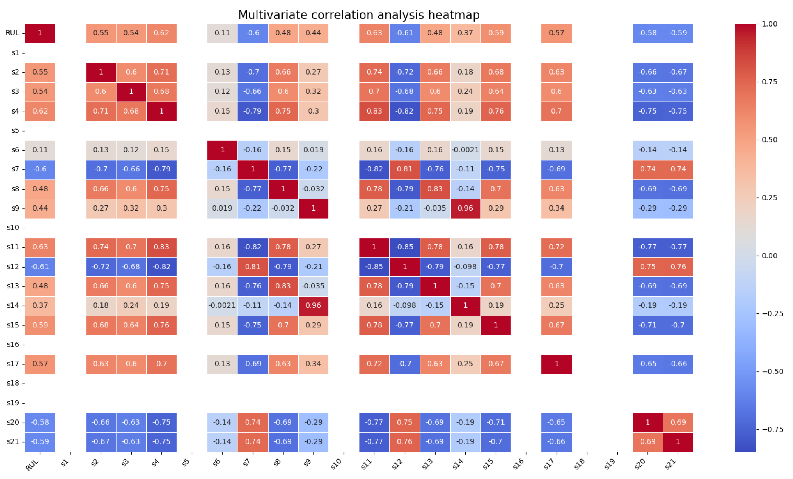
In real-world industrial applications, the contribution of data from different sensors to remaining useful life (RUL) prediction can vary significantly. Therefore, to ensure data quality, we performed an analysis on the 24 deployed sensors in the C-MAPSS dataset to remove those with poor correlation. Specifically, we analyzed the data collected from all sensors in the FD001 subset. As shown in Figure 7, the values of sensors S1, S5, S10, S16, S18, and S19 remain nearly constant throughout the entire lifecycle of the aircraft engine, indicating that these sensors have weak relevance to the RUL prediction task.
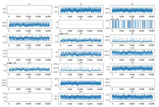
Figure 7.
Sensor value trends across the aircraft engine lifecycle.
Further confirmation was made by calculating the Pearson correlation coefficients between the sensor readings and RUL. As shown in Figure 8, the results confirm that sensors S1, S5, S10, S16, S18, and S19 have correlation coefficients close to 0 with RUL, verifying their weak contribution to the prediction task. Consequently, we selected sensors S2, S3, S4, S6, S7, S8, S9, S11, S12, S13, S14, S15, S17, S20, and S21 as inputs to our model.
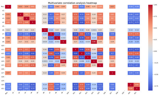
Figure 8.
Pearson correlation coefficients between sensor readings and RUL.
Furthermore, in the C-MAPSS dataset, the varying ranges of multiple types of sensor data resulted in significant differences in absolute values and magnitudes. To address this issue, we applied the Min-Max normalization strategy to scale all sensor values to the range of [−1, 1], eliminating scale differences. This ensures that high-value features do not disproportionately influence the model, while low-value features are not overlooked. Moreover, this normalization helps reduce floating-point errors in numerical calculations, improves numerical stability, and accelerates model convergence.
where represents the normalized data, X is the original data, and represent the maximum and minimum values in the data.
3.2.2. Slide Window
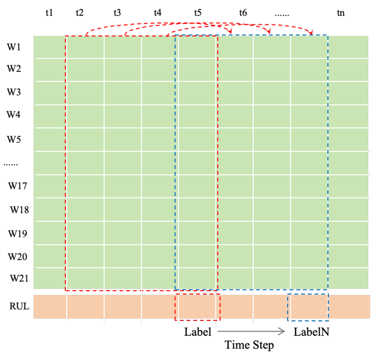
In time series data-related tasks, the primary focus is on analyzing the feature changes between adjacent data points of a variable at different time steps. A sliding window is often used as an effective method to extract useful features. In the C-MAPSS dataset, for the task of predicting the remaining useful life of engines, using data from multiple time steps typically captures more detailed degradation trend information compared to single time step data, significantly improving the model’s predictive performance, as illustrated in Figure 9.
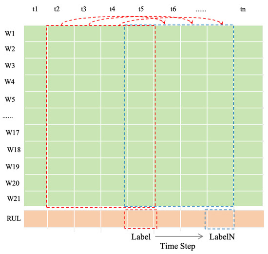
Figure 9.
The process of the sliding window.
3.2.3. RUL Label Reconstruction
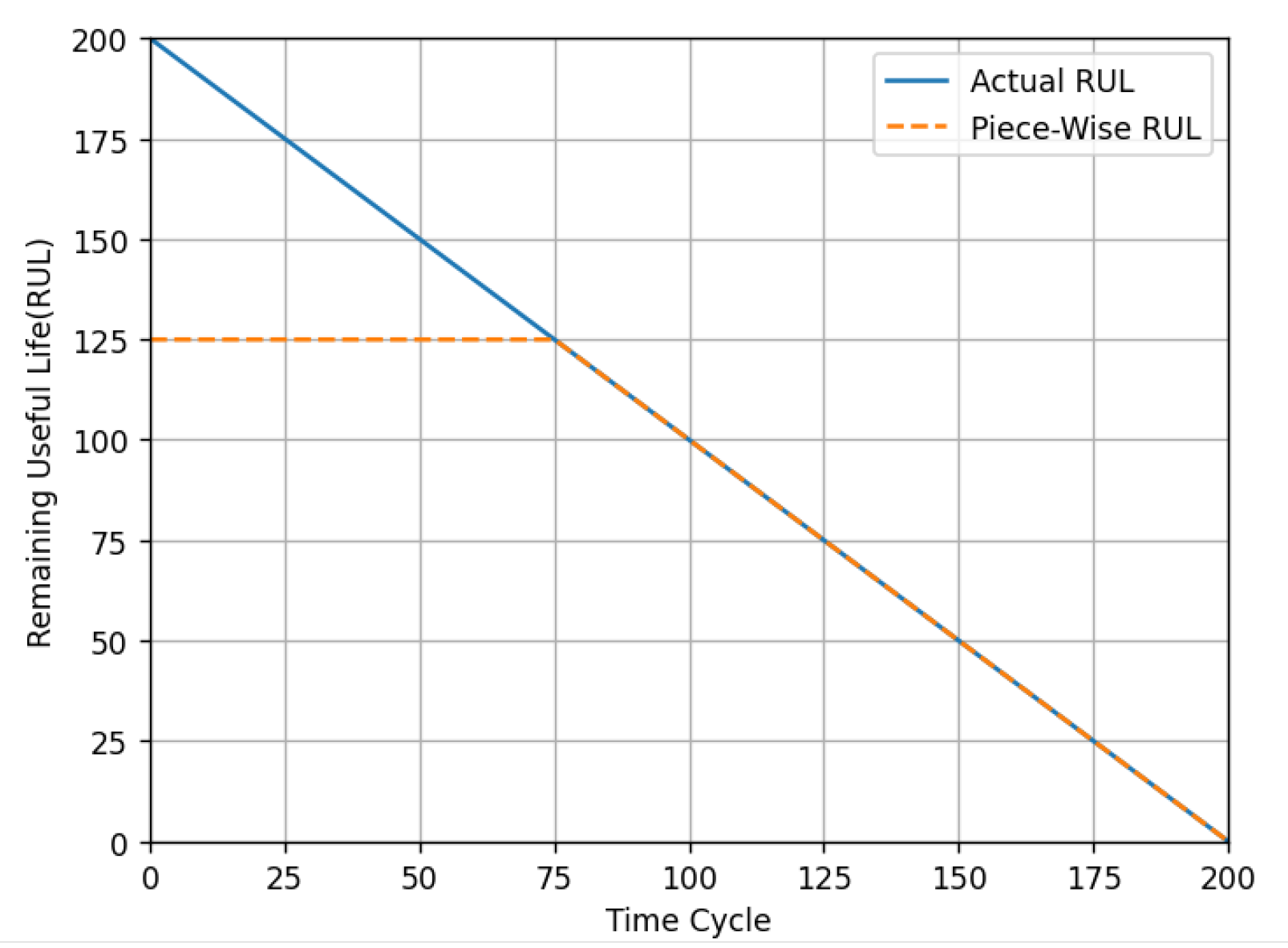
The entire lifecycle of the engine can be divided into two phases: the healthy phase and the degradation phase. During the healthy phase, the RUL remains at a relatively high and constant value, whereas in the degradation phase, the RUL declines significantly. To more effectively capture the engine’s lifecycle and provide more accurate RUL predictions, a piecewise linear model is employed. Multiple studies have validated that setting the RUL to 125 during the healthy phase is effective, and in this work, we adopt the same approach by setting the RUL to 125. After constructing samples using a sliding window approach, the RUL of the last cycle within each sample window is used as the label for that sample, as illustrated in Figure 10.
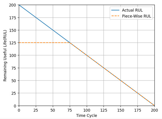
Figure 10.
Segmented linear function of RUL.
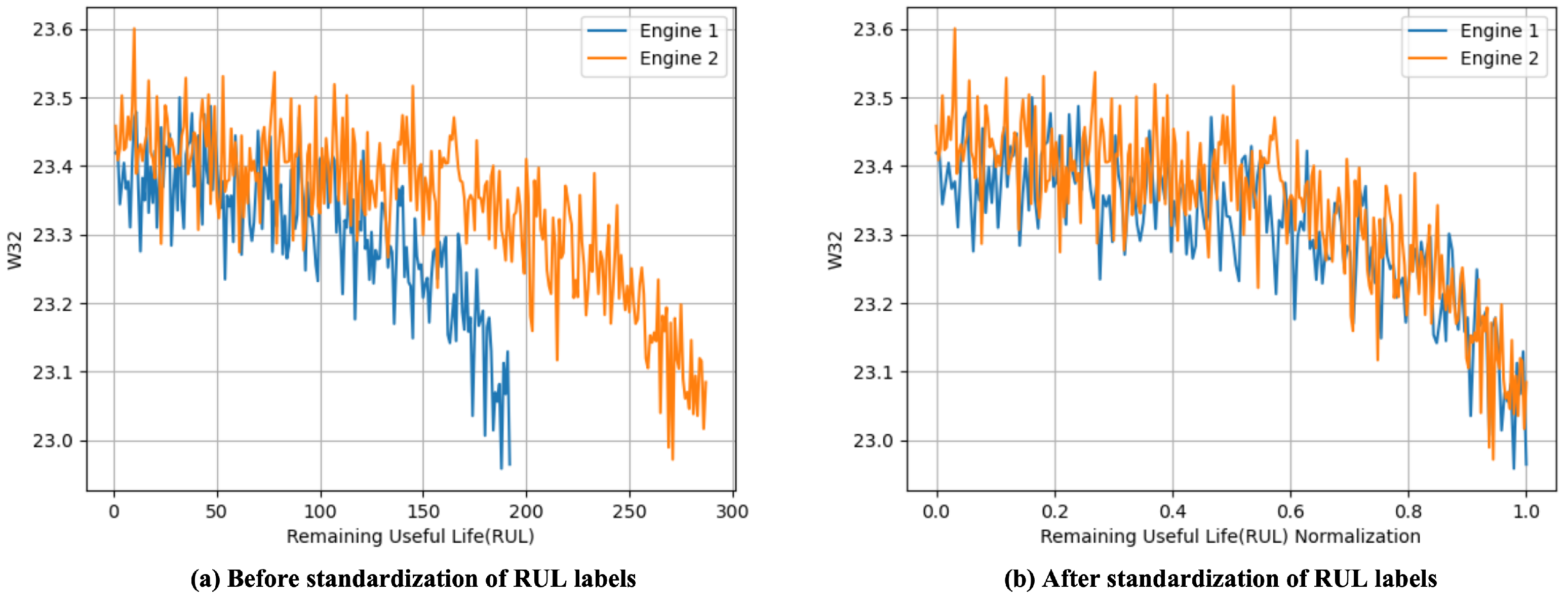
Additionally, to reduce the impact of varying degradation rates between different engines on model optimization, as shown in Figure 11, the RUL labels are standardized [25]. This involves transforming the RUL labels from specific absolute values (number of cycles) into relative proportions (RUL percentage). By doing so, samples with different degradation rates can be compared on the same scale, thereby enhancing the model’s generalization ability and improving optimization performance.
where is the standardized RUL label with the value range of [0, 1], and is the original RUL label, and is the maximum lifecycle of this engine.
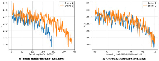
Figure 11.
The of Remaining Useful Life (RUL) Prediction with and without Label Standardization.
3.3. Hyperparameter Experiments
In this section, we study two key hyperparameters in the model: the window size and the number of DPI layers, and preliminarily verify the effectiveness of the model to explore the influence of hyperparameters under different complex working conditions.
The time window size W determines the length of the input data sequence that the model processes, directly influencing its ability to capture temporal dependencies. In related studies [11,12,23], it has been suggested to use W = 30 as the optimal window size for handling the C-MAPSS dataset to capture these dependencies. However, [29] tested various window sizes (1, 10, 20, 30, 40, 50, 60) to assess their impact on model performance, offering a broader range of options. Based on this, we adopt the values to explore the optimal W for our proposed model, with serving as the baseline for our experiments.
The number of DPI layers N controls the depth of feature extraction and the interaction between temporal and feature dimensions. In similar research [25], an in-depth exploration of N was conducted, testing values to determine their effect on model performance, with yielding the best results. Drawing from this work, we set the range of N to to investigate the optimal number of layers for our model, again using as the baseline.
Therefore, in our final setup, and , with and serving as the baseline model for the hyperparameter experiments. The root mean square error (RMSE) metric is used to identify the optimal combination of hyperparameters for our model.
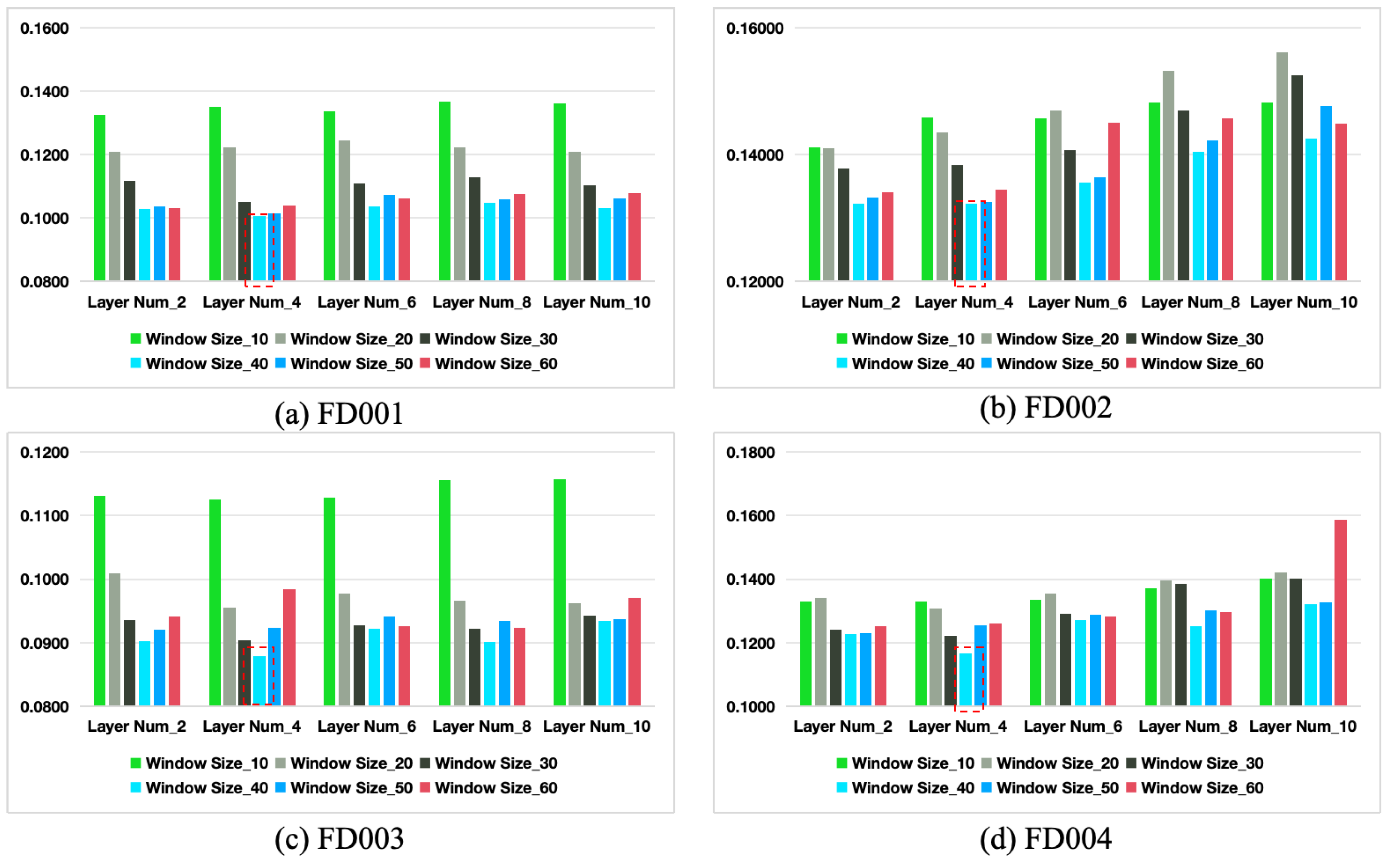
Based on the results in Table 4, when N is fixed, the RMSE metric first decreases and then increases as the window size W increases from 10 to 60. The model achieves the best performance across all four datasets when for the current number of DPI layers N. Similarly, when W is fixed, the RMSE also follows a similar trend of first decreasing and then increasing as N increases from 2 to 6. The model performs best across the four datasets when for the current window size W. Therefore, from a comprehensive analysis, the optimal parameter combination for our model is and . Compared to the baseline model (, ), the RMSE decreases by 12.70%, 6.47%, 7.33%, and 11.08% on the FD001, FD002, FD003, and FD004 datasets, respectively.

Table 4.
Experimental results of hyperparameter combinations for W and N.
Furthermore, as shown in Figure 12, the window size W directly influences the model’s ability to capture temporal features. Smaller window sizes may fail to capture long-term trends and dependencies, leading to reduced performance, particularly under complex operating conditions. On the other hand, if the window size W is too large, it may capture excessive temporal information, introducing unnecessary redundancy that increases computational complexity and the risk of overfitting, thereby reducing the mode’s generalization ability. Regarding the number of DPI layers N, this parameter controls the depth of feature extraction and the interaction between temporal and feature dimensions. With fewer layers, the model may be unable to adequately capture complex patterns in the data, negatively impacting performance. Conversely, too many layers may introduce noise and increase the risk of overfitting, thereby compromising generalization.
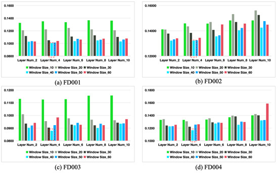
Figure 12.
The RMSE with different hyperparameters on the four datasets.
Thus, based on the experimental results for both window size W and the number of DPI layers N, an intermediate window size and an appropriate number of feature extraction layers enable the model to achieve optimal predictive performance without introducing redundancy or overfitting. The combination of and is identified as the optimal parameter setting for our model.
Therefore, all the hyperparameter settings adopted in the experiments of this paper are shown in Table 5.

Table 5.
Experimental hyperparameter configuration.
3.4. Comparison Experiments
In this chapter, we compare our method with state-of-the-art approaches in the field using the C-MAPSS dataset to validate the effectiveness of the model.
- LSTM [8]: A standard Long Short-Term Memory network for time series prediction.
- BTSAM [12]: A hybrid neural network that combines 1D Convolutional Neural Networks with Bidirectional Gated Recurrent Units in parallel.
- CNN-GRU [23]: A multi-dimensional feature fusion network that combines Convolutional Neural Networks and Gated Recurrent Units.
- DAMCNN [17]: A Deep Attention Mechanism Convolutional Neural Network designed to capture long-term dependencies in time series data.
- IMDSSN [11]: An Integrated Multi-head Dual Sparse Self-Attention Network (IMDSSN) based on an improved Transformer.
- MLP-Mixer [10]: A deep network architecture for multidimensional feature extraction that can be used for time series data.
- TS-Mixer [15]: A time series-based Mixer architecture designed to extract and mix features across multiple temporal windows.
- Dual-Mixer [25]: A dual-path feature extraction network that leverages the MLP-Mixer framework for parallel temporal and feature dimension interaction and extraction.
In addition, “-M” refers to the incorporation of the Multiscale Temporal-Feature Convolution Fusion Module, which is used to verify the effectiveness of this module. Models with the suffix indicate the inclusion of the MTF-CFM module, representing an improvement to the original model. The column labeled “Improvement” indicates the performance gains, with bold text highlighting the globally optimal performance metrics.
From Table 6, we can see that our proposed method achieved RMSE values of 0.0969, 0.1316, 0.086, and 0.1148 on the four datasets; MAPE values of 9.72%, 14.51%, 8.04%, and 11.27%; and Score values of 59.93, 209.39, 67.56, and 215.35. To comprehensively evaluate the performance of each model across all subsets, we calculated the average values for various metrics.

Table 6.
Comparative experiment results on C-MAPSS dataset.
- Compared to the second-best method, our proposed approach improved RMSE by 4.81%, 2.95%, 2.82%, and 7.64% across the four datasets, with an average improvement of 4.56%. For MAPE, the improvements were 8.47%, 12.91%, 5.74%, and 19.44%, with an average improvement of 11.64%. For the Score metric, the improvements were 2.43%, 5.06%, 4.35%, and 12.25%, averaging 6.02%.
- To validate the effectiveness of the MTF-CFM module, we computed the average improvements for all models across the four datasets. RMSE improved by 5.38%, 6.96%, 6.51%, and 9.63%, with an average improvement of 7.12%. For MAPE, the improvements were 8.51%, 13.18%, 9.53%, and 11.24%, averaging 10.62%. The Score metric improved by 5.09%, 7.78%, 6.44%, and 9.52%, with an average improvement of 7.21%.
These results demonstrate that our proposed model outperforms current state-of-the-art methods across all four datasets, with particularly strong performance on the more complex FD002 and FD004 datasets. This indicates that our model can more accurately predict RUL under complex conditions. Furthermore, the MTF-CFM module consistently enhances RUL prediction performance across all scenarios, showcasing its robustness and potential for wide applicability.
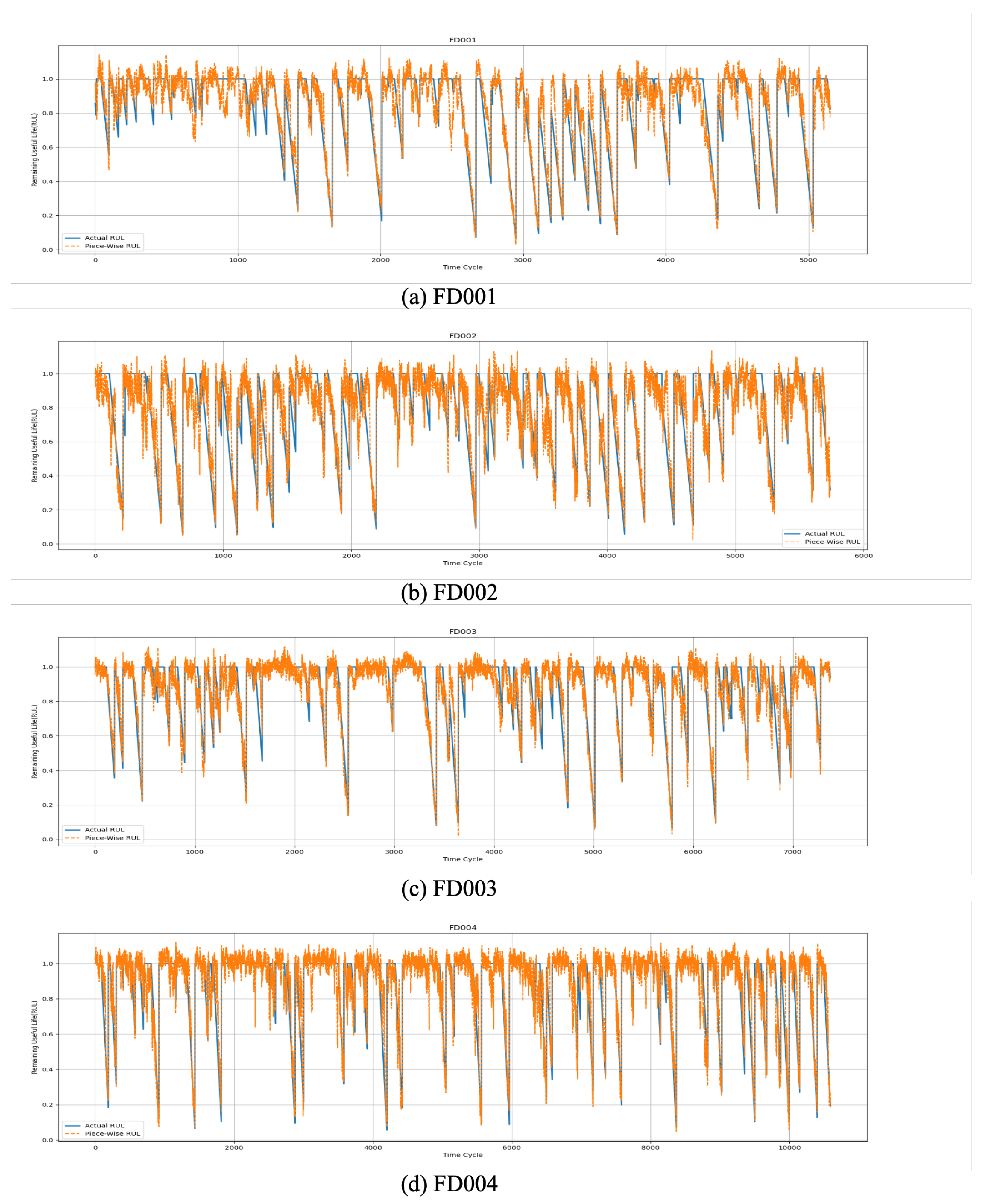
To provide a more intuitive demonstration of our algorithm’s performance on the C-MAPSS dataset, we conducted a visualization analysis comparing the actual and predicted RUL values for selected engines, as shown in Figure 13. From the figure, it can be observed that, aside from slight deviations at certain points, the predicted RUL values closely align with the actual RUL values in most cases. This result highlights the high accuracy of our proposed method in predicting engine RUL.
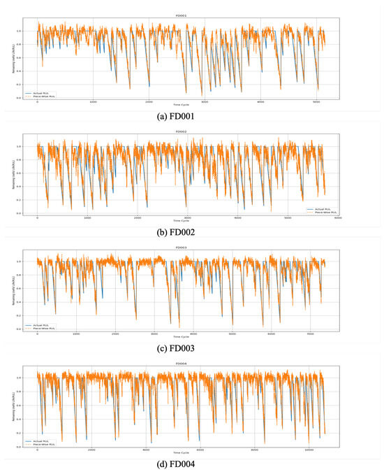
Figure 13.
Remaining useful life prediction on the C-MAPSS dataset.
To further supplement the explanation of the model parameters, we used the most complex FD004 dataset from the C-MAPSS dataset as an example, supplementing the experiment from three perspectives: the number of parameters, the model’s average running time, and memory usage.
According to Table 7, our proposed model demonstrates a balanced performance in terms of parameter count, average runtime, and memory usage. While the number of parameters in the proposed model (81,944) is slightly higher than some models, such as TS-Mixer (26,897), it remains significantly lower than the BTSAM model (2,824,528), indicating that our model strikes a good balance in terms of complexity. In terms of runtime, the proposed model averages 244.322 s, which, although slower than CNN-GRU (78.016 s) and DAMCNN (58.9 s), is notably more efficient than the more complex BTSAM model (377.798 s). Additionally, the proposed model exhibits moderate memory usage at 467 MiB, slightly exceeding TS-Mixer (349 MiB) and MLP-Mixer (340 MiB), but still demonstrating better memory efficiency than most other models.

Table 7.
Performance comparison of different models based on parameters, average running time, and memory usage.
Considering the inherent randomness of deep learning models, we conducted five repeated experiments for each dataset and included the standard deviation () in Table 6 to provide a more comprehensive evaluation. The standard deviation reflects the degree of dispersion in the results, offering insight into the model’s stability and consistency across different runs. From the distribution of values in Table 6, it is evident that our proposed model maintains relatively low RMSE and MAPE standard deviations across all four datasets. For instance, in the FD001 dataset, the RMSE is 0.0011, while in the FD004 dataset, it is 0.0029, indicating minimal fluctuation in prediction errors and high stability. In contrast, the CNN-GRU and IMDSSN models exhibit higher standard deviations, especially in the FD003 and FD004 datasets, where the larger variations in RMSE and MAPE values suggest less reliable performance under complex conditions. To further substantiate the effectiveness of the MTF-CFM module, we employed a t-test to compare the model’s performance before and after incorporating the module and treated the models with and without the MTF-CFM module as paired samples. After confirming that the differences between the paired samples follow a normal distribution, we performed a paired t-test using the following hypotheses:
Hypothesis 1.
: The MTF-CFM module has no effect on improving model performance.
Hypothesis 2.
: The MTF-CFM module has a significant effect on improving model performance.
The formula for the t-test is as follows:
where is the mean difference between the paired samples, is the standard deviation of the differences, is the number of paired observations.
In Table 8, with the exception of the MAPE metric for the CNN-GRU model, the test statistics for all other models are less than 0, indicating that the models incorporating the MTF-CFM module outperform those without it. Additionally, since p < 0.05, we reject the null hypothesis , at the significance level, accepting the alternative hypothesis . This confirms a statistically significant difference between the two models. Therefore, based on the provided metrics, the model with the MTF-CFM module demonstrates superior performance compared to the model without it.

Table 8.
The t-test results for FD004 Dataset.
3.5. Ablation Experiment
In this section, we design four sets of ablation experiments to validate the DPIN architecture, the MTF-CFM module, and the DWAM module within the model. We also analyze the effectiveness of the proposed MTF-CFM module in comparison to existing attention-based modules.
- DPIN-Del: This variant removes the feature interaction part of the dual-path network within the DPIN architecture, leaving only the dual-path outputs.
- DPIN: This is the baseline architecture of the model, designed to verify the importance of dual-path feature interaction by comparison with 1.
- DPIN-MTF-CFM: This variant combines the baseline architecture with the proposed MTF-CFM module, aiming to validate the effectiveness of the MTF-CFM module.
- DPIN-DWAM: This variant integrates the baseline architecture with the DWAM gating unit, aiming to verify the effectiveness of the DWAM unit.
- DPIN-MTF-CFM-DWAM: This represents the full architecture of the model, serving as the benchmark for the ablation experiment.
The experimental results in Table 9 show that after the interaction of the dual-path network, the model’s RMSE improved by an average of 4.40%, MAPE by 7.53%, and Score by 5.38%. This indicates that effective interaction between the time and feature dimensions is crucial for improving the accuracy and stability of RUL prediction.

Table 9.
Comparative ablation experiment results in C-MAPSS dataset.
After adding the MTF-CFM module, RMSE improved by an average of 2.76%, MAPE by 6.09%, and Score by 5.38%. These results demonstrate that the Multiscale Temporal-Feature Convolution Fusion Module significantly enhances the model’s ability to capture complex degradation patterns. When the DWAM module was added, RMSE improved by an average of 3.46%, MAPE by 4.96%, and Score by 5.30%, indicating that DWAM enables the model to dynamically adjust weights according to changes in the input features, thereby improving the model’s flexibility and adaptability when handling varying and complex equipment conditions.
When both the MTF-CFM and DWAM modules were integrated, RMSE improved by an average of 8.23%, MAPE by 19.63%, and Score by 11.88%. This comprehensive improvement suggests that the synergy between these two modules allows the model to achieve a higher level of performance in capturing multi-dimensional feature information and performing dynamic adjustments. This synergy significantly boosts the model’s prediction accuracy and stability, particularly in complex RUL prediction tasks.
Overall, these experimental results underscore the importance of feature interaction between the time and feature dimensions and validate the critical role of each proposed module in the overall model performance. Each module is indispensable, and their combination maximizes the performance of the RUL prediction model.
4. Discussion
The results of this study indicate that the proposed Dual-Path Interaction Network, combined with the MTF-CFM and DWAM modules, effectively enhances the model’s capability to capture complex degradation patterns and dynamically adjust to varying conditions. The significant improvements across multiple metrics—particularly in the FD002 and FD004 datasets, which represent more complex operational scenarios—highlight the robustness and flexibility of the model. The incorporation of multi-scale feature extraction and dynamic weight adaptation not only improves prediction accuracy but also provides better generalization across different conditions. However, the improvements are more pronounced in datasets with more complex conditions, suggesting that the model’s ability to handle simpler datasets could still be further optimized.
Moreover, while the ablation studies clearly demonstrate the contributions of each module, the model’s performance could benefit from additional enhancements in terms of computational efficiency and scalability. Future research could explore lightweight adaptations of the proposed modules to ensure that the model remains practical for real-time applications in industrial settings. Furthermore, exploring advanced techniques such as self-attention mechanisms or hybrid models could further improve the adaptability of the model across different RUL prediction tasks.
5. Conclusions
In this paper, we proposed a novel framework for remaining useful life prediction based on the Dual-Path Interaction Network. By integrating the Multiscale Temporal-Feature Convolution Fusion Module and the Dynamic Weight Adaptation Module, the model effectively captures complex patterns and dynamically adjusts to varying conditions in both time and feature dimensions. The proposed model was extensively tested on the C-MAPSS dataset, and the results showed that it outperforms state-of-the-art methods in RUL prediction tasks.
Through ablation experiments, we validated the individual contributions of the MTF-CFM and DWAM modules, confirming their effectiveness in enhancing the model’s prediction performance and stability. However, despite these improvements, the model has certain limitations, particularly in terms of computational efficiency and adaptability to simpler operational conditions. The current setup, with its parameter configuration, may result in higher computational costs, which can be further optimized, especially for scenarios where less complex models could suffice. In future research, we aim to address these limitations by improving computational efficiency and tailoring the model to better suit varied operational environments. We also plan to explore the application of the model in other industrial scenarios, such as predicting the lifetimes of key components in germ rice processing equipment. Additionally, we will investigate the use of transfer learning techniques to enhance the model’s generalization capabilities across different domains, thereby broadening its industrial applicability.
Author Contributions
Conceptualization, Z.L. and B.L.; methodology, Z.L.; validation, C.F. and J.W.; formal analysis, C.F.; data curation, L.X.; writing—original draft preparation, Z.L.; writing—review and editing, S.J.; visualization, H.Z.; project administration and funding acquisition B.L. All authors have read and agreed to the published version of the manuscript.
Funding
This work was supported in part by the following funding sources: The National Natural Science Foundation of China under Grant: 32472000. The Maior Scientific and Technological Achievements Transformation Proiect of Heilongjiang Province: CG18A006. The 2023 new round of ’double first-class’ discipline collaborative innovation results incubation project in Heilongjiang Province: LJGXCG2023-005.
Institutional Review Board Statement
Not applicable.
Informed Consent Statement
Not applicable.
Data Availability Statement
The original contributions presented in the study are included in the article; further inquiries can be directed to the corresponding author.
Acknowledgments
The authors would like to thank the Institute of Applied Electronics, China Academy of Engineering Physics for supporting this research project.
Conflicts of Interest
The authors declare no conflicts of interest.
References
- Liu, L.; Song, X.; Zhou, Z. Aircraft engine remaining useful life estimation via a double attention-based data-driven architecture. Reliab. Eng. Syst. Saf. 2022, 221, 108330. [Google Scholar] [CrossRef]
- Huang, C.; Bu, S.; Lee, H.H.; Chan, C.H.; Kong, S.W.; Yung, W.K. Prognostics and health management for predictive maintenance: A review. J. Manuf. Syst. 2024, 75, 78–101. [Google Scholar] [CrossRef]
- Shi, Y.; Cui, Y.; Cheng, H.; Li, L.; Li, X.; Kong, X. Multi-representation transferable attention network for remaining useful life prediction of rolling bearings under multiple working conditions. Meas. Sci. Technol. 2023, 35, 025037. [Google Scholar] [CrossRef]
- Zhang, Q.; Yang, P.; Liu, Q. A dual-stream spatio-temporal fusion network with multi-sensor signals for remaining useful life prediction. J. Manuf. Syst. 2024, 76, 43–58. [Google Scholar] [CrossRef]
- Ferreira, C.; Gonçalves, G. Remaining Useful Life prediction and challenges: A literature review on the use of Machine Learning Methods. J. Manuf. Syst. 2022, 63, 550–562. [Google Scholar] [CrossRef]
- Wu, F.; Wu, Q.; Tan, Y.; Xu, X. Remaining Useful Life Prediction Based on Deep Learning: A Survey. Sensors 2024, 24, 3454. [Google Scholar] [CrossRef]
- Khandelwal, K.S.; Shete, V.V. Design of regression neural network model for estimating the remaining useful life of lithium-ion battery. Intell. Decis. Technol. 2024, 18, 1615–1633. [Google Scholar] [CrossRef]
- Sayah, M.; Guebli, D.; Al Masry, Z.; Zerhouni, N. Robustness testing framework for RUL prediction Deep LSTM networks. ISA Trans. 2021, 113, 28–38. [Google Scholar] [CrossRef]
- Keshun, Y.; Guangqi, Q.; Yingkui, G. A 3D attention-enhanced hybrid neural network for turbofan engine remaining life prediction using CNN and BiLSTM models. IEEE Sens. J. 2023, 24, 21893–21905. [Google Scholar] [CrossRef]
- Tolstikhin, I.O.; Houlsby, N.; Kolesnikov, A.; Beyer, L.; Zhai, X.; Unterthiner, T.; Yung, J.; Steiner, A.; Keysers, D.; Uszkoreit, J.; et al. Mlp-mixer: An all-mlp architecture for vision. Adv. Neural Inf. Process. Syst. 2021, 34, 24261–24272. [Google Scholar]
- Zhang, J.; Li, X.; Tian, J.; Luo, H.; Yin, S. An integrated multi-head dual sparse self-attention network for remaining useful life prediction. Reliab. Eng. Syst. Saf. 2023, 233, 109096. [Google Scholar] [CrossRef]
- Zhang, J.; Jiang, Y.; Wu, S.; Li, X.; Luo, H.; Yin, S. Prediction of remaining useful life based on bidirectional gated recurrent unit with temporal self-attention mechanism. Reliab. Eng. Syst. Saf. 2022, 221, 108297. [Google Scholar] [CrossRef]
- Li, Y.; Chen, Y.; Shao, H.; Zhang, H. A novel dual attention mechanism combined with knowledge for remaining useful life prediction based on gated recurrent units. Reliab. Eng. Syst. Saf. 2023, 239, 109514. [Google Scholar] [CrossRef]
- Chen, S.; He, J.; Wen, P.; Zhang, J.; Huang, D.; Zhao, S. Remaining Useful Life Prognostics and Uncertainty Quantification for Aircraft Engines Based on Convolutional Bayesian Long Short-Term Memory Neural Network. In Proceedings of the 2023 Prognostics and Health Management Conference (PHM), Paris, France, 31 May–2 June 2023; pp. 238–244. [Google Scholar]
- Ekambaram, V.; Jati, A.; Nguyen, N.; Sinthong, P.; Kalagnanam, J. Tsmixer: Lightweight mlp-mixer model for multivariate time series forecasting. In Proceedings of the 29th ACM SIGKDD Conference on Knowledge Discovery and Data Mining, Long Beach, CA, USA, 6–10 August 2023; pp. 459–469. [Google Scholar]
- Zhao, L.; Song, S.; Wang, P.; Wang, C.; Wang, J.; Guo, M. A MLP-Mixer and mixture of expert model for remaining useful life prediction of lithium-ion batteries. Front. Comput. Sci. 2024, 18, 185329. [Google Scholar] [CrossRef]
- Jiang, F.; Ding, K.; He, G.; Lin, H.; Chen, Z.; Li, W. Dual-attention-based multiscale convolutional neural network with stage division for remaining useful life prediction of rolling bearings. IEEE Trans. Instrum. Meas. 2022, 71, 3525410. [Google Scholar] [CrossRef]
- Wang, J.; Wang, Y.; Li, J. Interpretable and efficient RUL prediction of turbofan engines using EM-enhanced Bi-LSTM with TCN and attention mechanism. Eng. Res. Express 2024, 6, 035507. [Google Scholar] [CrossRef]
- Mao, S.; Li, X.; Zhao, B. Remaining useful life prediction based on time-series features and conformalized quantile regression. Meas. Sci. Technol. 2024, 35, 126113. [Google Scholar] [CrossRef]
- Lei, Z.; Su, Y.; Feng, K.; Wen, G. Interpretable operational condition attention-informed domain adaptation network for remaining useful life prediction under variable operational conditions. Control. Eng. Pract. 2024, 153, 106080. [Google Scholar] [CrossRef]
- Wang, H.; Li, D.; Li, Y.; Zhu, G.; Lin, R. Method for Remaining Useful Life Prediction of Turbofan Engines Combining Adam Optimization-Based Self-Attention Mechanism with Temporal Convolutional Networks. Appl. Sci. 2024, 14, 7723. [Google Scholar] [CrossRef]
- Ren, X.; Qin, Y.; Li, B.; Wang, B.; Yi, X.; Jia, L. A core space gradient projection-based continual learning framework for remaining useful life prediction of machinery under variable operating conditions. Reliab. Eng. Syst. Saf. 2024, 252, 110428. [Google Scholar] [CrossRef]
- Zhang, J.; Tian, J.; Li, M.; Leon, J.I.; Franquelo, L.G.; Luo, H.; Yin, S. A parallel hybrid neural network with integration of spatial and temporal features for remaining useful life prediction in prognostics. IEEE Trans. Instrum. Meas. 2022, 72, 3501112. [Google Scholar] [CrossRef]
- Remadna, I.; Terrissa, S.; Sayah, M.; Ayad, S.; Zerhouni, N. Boosting RUL prediction using a hybrid deep CNN-BLSTM architecture. Autom. Control. Comput. Sci. 2022, 56, 300–310. [Google Scholar] [CrossRef]
- Fu, E.; Hu, Y.; Peng, K.; Chu, Y. Supervised Contrastive Learning based Dual-Mixer Model for Remaining Useful Life Prediction. arXiv 2024, arXiv:2401.16462. [Google Scholar] [CrossRef]
- Zhang, Y.; Liu, K.; Zhang, J.; Huang, L. Self-attention Mechanism Network Integrating Spatio-Temporal Feature Extraction for Remaining Useful Life Prediction. J. Electr. Eng. Technol. 2024, 1–16. [Google Scholar] [CrossRef]
- Deng, S.; Zhou, J. Prediction of remaining useful life of aero-engines based on CNN-LSTM-Attention. Int. J. Comput. Intell. Syst. 2024, 17, 232. [Google Scholar] [CrossRef]
- Dong, L.; Jian, S.; Zirui, L.; Haoyu, G. Prognostics and health management for electromechanical system: A review. J. Adv. Manuf. Sci. Technol. 2022, 2, 2022015. [Google Scholar]
- Lai, Z.; Liu, M.; Pan, Y.; Chen, D. Multi-dimensional self attention based approach for remaining useful life estimation. arXiv 2022, arXiv:2212.05772. [Google Scholar]
Disclaimer/Publisher’s Note: The statements, opinions and data contained in all publications are solely those of the individual author(s) and contributor(s) and not of MDPI and/or the editor(s). MDPI and/or the editor(s) disclaim responsibility for any injury to people or property resulting from any ideas, methods, instructions or products referred to in the content. |
© 2024 by the authors. Licensee MDPI, Basel, Switzerland. This article is an open access article distributed under the terms and conditions of the Creative Commons Attribution (CC BY) license (https://creativecommons.org/licenses/by/4.0/).

