Abstract
Piezoelectric actuators (PEAs) are extensively used for scanning and positioning in scanning probe microscopy (SPM) due to their high precision, simple construction, and fast response. However, there are significant challenges for instrument designers due to their nonlinear properties. Nonlinear properties make precise and accurate control difficult in cases where position feedback sensors cannot be employed. However, the performance of PEA-driven scanners can be significantly improved without position feedback sensors if an accurate mathematical model with low computational costs is applied to reduce hysteresis and other nonlinear effects. Various methods have been proposed for modeling PEAs, but most of them have limitations in terms of their accuracy and computational efficiencies. In this research, we propose a variant DenseNet-type neural network (NN) model for modeling PEAs in an AFM scanner where position feedback sensors are not available. To improve the performance of this model, the mapping of the forward and backward directions is carried out separately. The experimental results successfully demonstrate the efficacy of the proposed model by reducing the relative root-mean-square (RMS) error to less than 0.1%.
1. Introduction
High-speed atomic force microscopy (HS-AFM) is one of the most powerful tools used to measure the topographic properties of various materials at the nanoscale with high resolution and speed [1,2]. Three-dimensional topography can also be captured by scanning a sample surface with a sharp tip attached to a cantilever and by measuring the interaction between the tip and the surface. The performance of HS-AFM is significantly impacted by the particularity of its instrumental components, with the nano-positioning stage directly affecting imaging [3,4].
Piezoelectric actuators (PEAs) are commonly utilized devices for controlling extremely small-scale positioning due to their high precision, high-speed response, large actuation force, and ease of integration [5,6,7]. In HS-AFM, PEAs are used to scan the AFM tip across the sample surface in a controlled manner that allows for the quick data acquisition required for high-speed imaging. Despite their advantages and widespread applications, all PEAs intrinsically exhibit nonlinearity properties, such as creep and hysteresis, which can considerably degrade the accuracy in nano-positioning. Hysteresis is easily the most complex, laborious, and concerning nonlinear characteristic, as it causes deviations in the achieved motion from the desired motion in a nano-positioning system. Hence, minimizing the effects of hysteresis is extremely important [5,6,8]. The hysteresis behavior of piezoelectric actuators is described using hysteresis models, such as physics-based and data-based phenomenological models. However, in addition to the hysteresis caused by the physical properties of the material, it also depends on the rate of the input signal, which makes the compensation process much more complicated [9,10]
Over the years, several approaches have been proposed to overcome the impact of hysteresis and to enhance the performance of PEAs. They can be categorized in three groups: (1) feedback control, (2) model-based feedforward compensation, and (3) combined feedback and feedforward control. In feedback control, positioning is monitored and compensated by added position feedback sensors to adjust the control signal based on the difference between the desired output and the actual output. Effects due to hysteresis can be significantly reduced through closed-loop feedback control. However, the effectiveness of this method is limited by the noise in the position feedback sensors and the bandwidth of PEAs, especially in systems with large delays or high control gains [11,12,13]. Feedforward–feedback controllers have been applied in several recent studies due to their high accuracy [5,8,14]. However, this method still requires expensive position feedback sensors. In this regard, a model-based feedforward compensation is the optimal alternative for compromising between costs, performance, and stability requirements. The basic concept of feedforward compensation is to construct a mathematical model to simulate the nonlinearity of PEAs and then reshape the input to linearize the output, thus resulting in a more precise and effective control [15].
The most important factor affecting the performance of feedforward control is how close a given model for hysteresis is to the actual hysteresis of the PEAs used [16]. Some of widely used models for compensation are Bouc–Wen (BW), Preisach, Prandtl–Ishlinskii (PI), and intelligent algorithms. Although widely used, the effectiveness of these aforementioned models is often limited due to limitations such as high computational costs and difficulty in deriving their inverse hysteresis models [5,7,14].
Recently, researchers have started to apply techniques associated with artificial neural network (ANNs) to feedforward compensation. A major benefit of using ANNs is their capacity to effectively model complex and nonlinear relationships between input and output variables. Their high flexibility and adaptability allow neural networks to learn and adapt to different input data without having to manually adjust parameters, thereby providing accurate results in a wide range of applications. In [1], a feedforward multi-layer neural network is used to shape a proper control signal based on the expected output. Another example of a multi-layer neural network is proposed in [17] where the authors used a multi-layer feedforward neural network-based inverse hysteresis model to increase the bandwidth of the system up to 1000 Hz. In [18], an online neural-network-based sliding mode control is utilized to obtain a robust, precise adaptive control for the piezoelectric tube scanner. The authors of [6] used a feedback controller combined with a Hammerstein–Wiener model to eliminate the hysteresis effect and enhance the PEA performance.
Although artificial neural networks are a powerful tool for dealing with nonlinear problems, they still have some limitations when using a simple fully connected neural network (FCNN) structure. In complicated problems that need a deep neural network such as modeling PEAs, increasing the number of layers can lead to the gradient vanishing problem, where the model cannot effectively learn from data to adjust its weights.
In this research, a variant DenseNet-type neural network model is proposed to deal with the nonlinear behaviors of PEAs. The concept behind a DenseNet is to enhance the information flow inside the architecture by using skip connections, thereby giving this method the ability to make decisions based on all layers instead of the last layer. A skip connection is a shortcut that allows information to bypass any intermediate layer to be added directly to the output of the preceding layer. This, in turn, facilitates the flow of information in the network and helps to address the issue of gradient vanishing during training and to enhance the model accuracy. Considering that the complexity of the problem is directly proportional to the number of layers and neurons in the neural network, a multi-model approach with a dense neural network is applied to model each PEA. This approach involves calculating each forward and backward movement based on distinct models, thereby simplifying the modeling process compared to incorporating both the forward and backward movements of a PEA into a single model.
2. Materials and Methods
2.1. Materials and Experimental Setup
The schematic of the experimental setup to analyze the hysteresis of PEAs is shown in Figure 1.
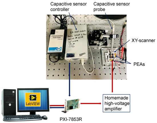
Figure 1.
Experimental setup used to collect data for analyzing the hysteresis of the piezoelectric actuator.
The Thorlab PK4FQP2 PEA used in this study is a discrete piezoelectric stack made from lead zirconate titanate (PZT) ceramic. It is made up of piezoelectric chips bonded with glass beads and epoxy. The displacement at the maximum drive voltage provided is 20 µm ± 15%, according to the manufacturer. The characteristics of the Thorlab PK4FQP2 are shown in Table 1.

Table 1.
Thorlab PK4FQP2 piezoelectric stack specifications.
The PEAs are arranged symmetrically to the supporting base of a homemade XY scanner (maximum XY scan range ∼27 × 27 μm2) and drive the supporting base in the X (fast direction) and Y (slow direction) axes, respectively.
A homemade high-voltage amplifier with a small signal bandwidth of 110 kHz and an output current of 200 mA is used to drive the PEAs. The output displacement of the XY scanner is measured by using a capacitive sensor (5504, MicroSense, LLC, Lowell, MA, USA) and its gauging module (5810, MicroSense, LLC, Lowell, MA, USA). The output signal from the capacitive sensor module is acquired and displayed by using a field programmable gate array (FPGA) module with real-time input/output (RIO) (PXI-7853R, National Instruments, Austin, TX, USA). The PEA’s response is measured after the triangular input signals with different amplitudes (25 V, 50 V, 75 V, and 100 V) are used to drive each axis. Figure 2 shows the relationship between the input voltage and the output displacement of the scanner. We collected 2000 samples for each trajectory (1000 samples each for forward and backward directions) for different amplitude inputs. The whole experimental procedure was repeated 20 times to reduce measurement errors.
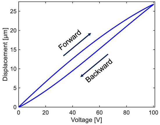
Figure 2.
Hysteresis curve between the input voltage and the displacement for the X-axis of the homemade scanner.
2.2. DenseNet-Type Neural Network Model
An artificial neural network (ANN) is a type of computer programming where instead of manually coding a set of rules, a programmer enables the computer to learn from data and to build the rules itself. Although in most cases the rules may be unclear, the computer gains the ability to make new decisions based on the input data and the learned rules. There are many types of ANN models designed for specific purposes, such as convolutional neural networks (CNNs) and recurrent neural networks (RNNs) suitable for image and language processing, respectively. Among the various neural networks, fully connected neural networks (FCNNs) (Figure 3) have been very popular. An FCNN comprises interconnected artificial neurons arranged in sequential layers. Each neuron aggregates inputs from other neurons, processes them to generate an output, and then passes this output to subsequent neurons in the network. Although an FCNN is utilized as a useful tool for prediction and classification, its accuracy is restricted by problems related to the number of neurons and layers in the hidden layer. In other words, the number of neurons and layers significantly impacts the network performance. Too few hidden connections will hinder the learning process, while too many layers inside the model will cause a vanishing gradient issue when the network is trained by using the back-propagation learning rule in a deep neural network [19,20,21].
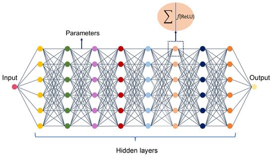
Figure 3.
Structure of a fully connected layer model.
Some common models have focused on mitigating the effects of the vanishing gradient problem, including using a rectified linear unit (ReLU) as an activation function [22,23], a residual neural network (ResNet) [24,25], or a densely connected convolutional network (DenseNet) [26,27]. ReLU is a fairly simple and effective activation function. Having a gradient of 0 or 1 makes ReLU less susceptible to the vanishing gradient problem. By using skip connections, ResNet can deal with the vanishing gradient problem to some extent. However, ResNet is not effective in deep neural networks [28]. DenseNet is a method that has been used in many studies to achieve a higher accuracy in image processing [29,30,31]. The structure of DenseNet is quite similar to that of ResNet. Whereas ResNet employs an additional operator to pass the information from the previous layer to a deeper layer, DenseNet uses concatenation to combine the previous layer with all deeper layers. These concatenated layers bring the information from the input to every layer inside the model and finally to the output. This causes the output to be directly affected by every layer inside the model, solving the problem of gradient vanishing.
A DenseNet-type neural network model includes three primary parts: an input layer, hidden layers, and an output layer. The purpose of the input layer is to receive the data and then to send them to the hidden layers to start the training process. In this research, the hidden layers are designed with eight inner layers and six artificial neurons in each layer. Each artificial neuron receives inputs from all the neurons in the previous layer according to their weights (w) and biases (b) and then passes the results through an activation function, as shown in Figure 4. The performed calculation is represented in the form of a transfer function:
where , f, , and b are the input, activation function, weight, and bias at an artificial node and its connection, respectively. n is the total number of neurons in the previous layer. The information is transmitted through the network by repeating the above calculation for each layer until it reaches the output node.
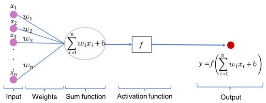
Figure 4.
Mathematical formulation behind an ANN node.
The ReLU function applied as an activation function in this network is given as follows:
The proposed model is an unclear function that represents the relationship between the position and the voltage, expressed as below:
where F is the transfer function of the PEA defined by the DenseNet model structure. This transfer function determines how the neural network utilizes input information to produce the output by performing calculations based on weights and biases and then passing it through an activation function to transmit information.
Eliminating some connections in the network does not reduce the accuracy of the model. It also improves the computational time and cost. Therefore, a variant of the DenseNet structure was applied in this study to deal with the nonlinear problem of the PEAs. Instead of using all the shortcuts in a DenseNet, we only use the shortcuts shown in Figure 5 as the model structure.
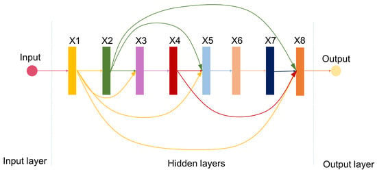
Figure 5.
Structure of the variant DenseNet-type fully connected model.
2.3. Identification Process
Figure 6 illustrates the flow chart of building a mathematical model to solve the nonlinear problems of the PEAs using a DenseNet-type artificial neural network. This process includes four steps:
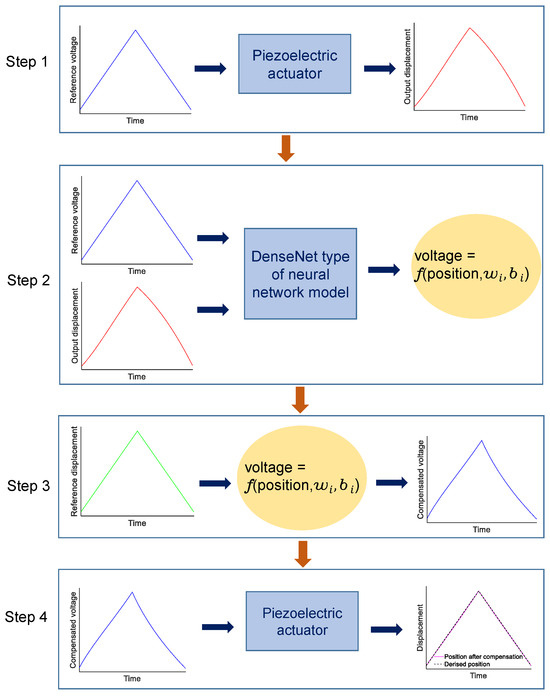
Figure 6.
Identification process.
- Step 1:
- Data collection.In this step, a triangular-wave control signal with a sampling frequency of 1 Hz is applied to the PEAs to obtain the relationship between the control signal and the position of the PEAs.
- Step 2:
- Train the neural network model using the collected data.Before the training process, each dataset is randomly separated into two parts: 80% and 20% of the original datasets are used for training and testing, respectively. Then, the datasets are continuously divided into two parts: trace and retrace. To enhance the accuracy of the control framework, modeling is performed separately for trace and retrace. To minimize the sensor and/or measurement errors, the data used for training is averaged from 10 separate measurements. Training begins by initializing random weights and biases for all nodes inside the model. The model then uses gradient descent (GD) as an optimization algorithm to adjust these weights and biases so that the error between the predicted and expected results is minimized. The function that represents the difference between the predicted results and the actual data is called the loss function. In this work, the mean squared error (MSE) shown in Equation (3) is employed as the loss function.where m represents the number of samples in a dataset. and are the actual output and predicted output of the instance, respectively. The weight and bias are updated as shown below:where k is the training iteration and n is the learning rate. After the model training process finishes, the model structure and a set of parameters including weights and biases are saved for the next step. The training for each forward/backward direction at each amplitude lasts for about 20 min with 12,000 epochs for 100 V, 9000 epochs for 75 V, 7000 epochs for 50 V, and 5000 epochs for 25 V. TensorFlow, a powerful and flexible library in machine learning and artificial intelligence, is used to build and train the hidden layer. The entire process in this step is performed in the Google Colaboratory framework.
- Step 3:
- Generate the compensated control signal.In this step, the reference data (expected position) are passed through the model obtained in Step 2. This process is performed in Python. The output of the model is a set of compensated control signals corresponding to each input reference data
- Step 4:
- Drive the PEAs using the compensated signal.
2.4. Performance Metrics
To facilitate the evaluation of the quality of the trained model and the performance of the control framework, the root mean squared error (RMSE) and relative root mean squared error (RRMSE) are calculated as below:
where N is the length of the analyzed data. and represent the actual result and the predicted/desired result at sample, respectively.
3. Results and Discussion
3.1. Fitting of Hysteresis Curve by the Proposed Artificial Neural Network Model
Figure 7 illustrates the fitting of the ANN model for the hysteresis measured at amplitudes of 25 V, 50 V, 75 V, and 100 V for (a) the X-axis and (b) the Y-axis. The accuracy of the proposed ANN model for each axis is assessed and shown in Table 2. For the X-axis, the RMSE is less than 0.05 m and the RRMSE is less than 0.08% for all amplitudes. For the Y-axis, the RMSE is less than 0.06 m and the RRMSE is less than 0.1% for all amplitudes.
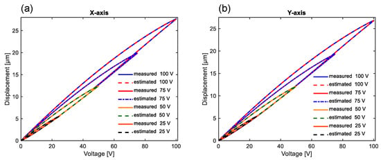
Figure 7.
Hysteresis curves fitted with a DenseNet-type neural network for (a) the X-axis and (b) the Y-axis.

Table 2.
Metrics for the X- and Y-axes calculated for different driving amplitudes.
3.2. Compensation Result
A custom-written LabVIEW code in combination with the trained model is utilized to drive the PEAs. Then, the achieved displacement is measured to check how well the overall compensation scheme works. Figure 8 shows the uncompensated displacements, desired trajectories, and compensated displacements (left) and the corresponding hysteresis error (right) of the X- and Y-axes for different driving voltages.
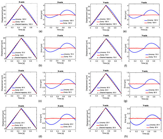
Figure 8.
Comparison of uncompensated/compensated trajectories with desired trajectories (left) and hysteresis error (right) for different driving voltages: (a) 100 V, (b) 75 V, (c) 50 V, (d) 25 V for the X-axis and (e) 100 V, (f) 75 V, (g) 50 V, (h) 25 V for the Y-axis.
The performance of the control framework is evaluated by using the RMSE and RRMSE as metrics calculated based on the deviations of the uncompensated/compensated trajectories from the desired trajectory, and the results are presented in Table 3. The RMSE values of both the X- and Y- axes show a significant decrease after the compensation process. The RRMSE values also show a substantial improvement. Compared to other methods, such as PI [32,33] and BW [34], which have RRMSE values of about 1%, a simple neural network model using a polynomial algorithm has RRMSE values of 1.59% [35], and a feedback-combined Hammerstein–Wiener model has RRMSE values of 0.38%) [6]. Our proposed method provides relatively high precision for piezo control, thereby significantly enhancing the efficiency of the system’s performance.

Table 3.
Metrics calculated for the X- and Y-axes to evaluate the performance of the control framework.
3.3. AFM Imaging
To investigate the performance of the proposed model applied to AFM imaging, we acquired tapping mode images of DVD data tracks with a homemade tip-scanning AFM. Unlike conventional sample scanning AFM systems, where a cantilever remains stationary while the sample under investigation is raster scanned by an XY-scanner, in our AFM system, the XY-scanner is attached to the AFM head and the cantilever is mounted on the supporting base of the XY-scanner. The cantilever is moved with the supporting base through the control of the PEAs, while the sample remains stationary. A Bruker RTESP-300 cantilever with a resonance frequency of 300 kHz is used to obtain images in tapping mode. A custom-written LabVIEW real-time code is utilized to control the AFM and to collect data. All images are of a scan size of about 5.5 m by 5.5 m at a resolution of 256 pixels by 256 pixels.
For the initial test, we collect images at a scan frequency of 1 Hz. The tapping mode images of DVD data tracks in trace and retrace directions are collected by our homemade tip-scanning AFM without compensation, as illustrated in Figure 9a,b, respectively. As observed in Figure 9c, the line profiles in the trace and retrace images show size distortions and position offsets due to the nonlinearities of the PEAs used in the scanner. For comparison, images obtained with the linearized scanner are shown in Figure 9d,e. The trace and retrace images are visually matching, and the distortions are significantly reduced. The line profiles shown in Figure 9f are nearly identical, clearly demonstrating that the linearization of the PEA-driven scanner is successfully achieved.
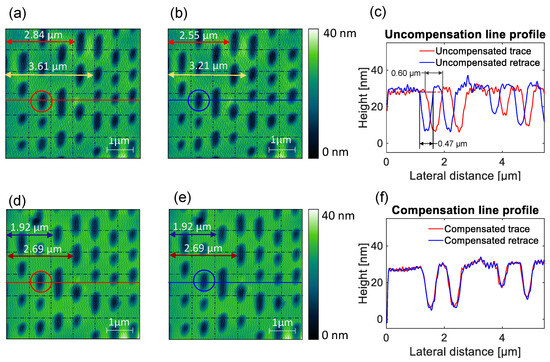
Figure 9.
Tapping mode images of DVD data tracks obtained at 1 Hz with (a) an uncompensated scanner (trace) and (b) an uncompensated scanner (retrace). (c) A line profile for the red and blue lines in (a,b). Tapping mode images of DVD data tracks obtained at 1 Hz with(d) a compensated scanner (trace) and (e) a compensated scanner (retrace). (f) A line profile for the red and blue line in (d,e).
Our proposed model is also applied to higher scanning frequencies. Figure 10 shows the AFM images of DVD data tracks obtained with the compensated and uncompensated scanner operated at 5 Hz and 30 Hz. At high frequencies, edges in the images begin to show the effects of scanner vibrations caused by the sudden momentum change in the scanner movement when driven by a triangular waveform. However, the near absence of distortions and position offsets in the trace and retrace images clearly demonstrates the effectiveness of our proposed DenseNet-type neural network for PEA compensation.
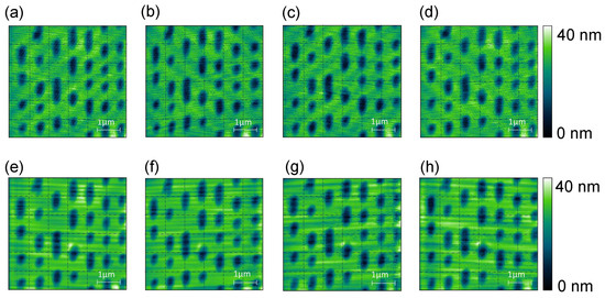
Figure 10.
Tapping mode images of DVD data tracks obtained at 5 Hz with (a) an uncompensated scanner (trace), (b) an uncompensated scanner (retrace), (c) a compensated scanner (trace), and (d) a compensated scanner (retrace), and at 30 Hz with (e) an uncompensated scanner (trace), (f) an uncompensated scanner (retrace), (g) a compensated scanner (trace), and (h) a compensated scanner (retrace).
4. Conclusions
In this work, we have successfully applied a neural network model to solve the problem of PEA modeling. With the adaptability of neural networks and a clever approach to designing a model structure, we have achieved high accuracy in modeling our piezo device compared to other existing methods such as PI, BW, or other traditional methods. In doing so, we successfully compensated for the highly nonlinear properties of PEAs. Furthermore, we have applied the results from the NN modeling to obtain images of DVD data tracks. Analyses of the obtained images clearly demonstrate the effectiveness of our proposed method in linearizing nonlinear PEA-driven scanners at various frequencies.
Author Contributions
Conceptualization, T.T.N. and Y.J.L.; methodology, T.T.N.; software, T.T.N. and L.O.O.; hardware, T.T.N.; validation, T.T.N.; formal analysis, T.T.N.; data curation, T.T.N.; writing—original draft preparation, T.T.N., O.M.J. and T.N.N.; review and editing, Y.J.L.; supervision, Y.J.L.; project administration, Y.J.L.; funding acquisition, Y.J.L. All authors have read and agreed to the published version of the manuscript.
Funding
This work is supported by Basic Science Research Program through the National Research Foundation of Korea (NRF) funded by the Ministry of Education (NRF-2021R1I1A3056881).
Institutional Review Board Statement
Not applicable.
Informed Consent Statement
Not applicable.
Data Availability Statement
The original contributions presented in this study are included in this article, and further inquiries can be directed to the corresponding authors.
Conflicts of Interest
The authors declare no conflicts of interest.
References
- Othman, Y.S.; Mahmood, I.A.; Rashid, N.K.A.M.; Darsivan, F.J. Artificial neural network based hysteresis compensation for piezoelectric tube scanner in atomic force microscopy. In Proceedings of the TENCON 2012 IEEE Region 10 Conference, Cebu, Philippines, 19–22 November 2012; pp. 1–5. [Google Scholar]
- Javazm, M.R.; Pishkenari, H.N. Observer design for topography estimation in atomic force microscopy using neural and fuzzy networks. Ultramicroscopy 2020, 214, 113008. [Google Scholar] [CrossRef]
- Tao, Y.D.; Li, H.X.; Zhu, L.M. Hysteresis modeling with frequency-separation-based Gaussian process and its application to sinusoidal scanning for fast imaging of atomic force microscope. Sens. Actuator A Phys. 2020, 311, 112070. [Google Scholar] [CrossRef]
- Asmari, N.; Kangül, M.; Andany, S.H.; Karimi, A.; Fantner, G.E. Data-Driven Feedforward Hysteresis Compensation with Genetic Algorithm for Atomic Force Microscope. In Proceedings of the 2022 International Conference on Manipulation, Automation and Robotics at Small Scales (MARSS), Toronto, ON, Canada, 25–29 July 2022; pp. 1–6. [Google Scholar]
- Napole, C.; Barambones, O.; Calvo, I.; Velasco, J. Feedforward compensation analysis of piezoelectric actuators using artificial neural networks with conventional PID controller and single-neuron PID based on Hebb learning rules. Energies 2020, 13, 3929. [Google Scholar] [CrossRef]
- Napole, C.; Barambones, O.; Calvo, I.; Derbeli, M.; Silaa, M.Y.; Velasco, J. Advances in tracking control for piezoelectric actuators using fuzzy logic and hammerstein-wiener compensation. Mathematics 2020, 8, 2071. [Google Scholar] [CrossRef]
- Soares Barbosa, M.P.; Rakotondrabe, M.; Hultmann Ayala, H.V. Deep learning applied to data-driven dynamic characterization of hysteretic piezoelectric micromanipulators. In Proceedings of the 21st IFAC World Congress, Berlin, Germany, 11–17 July 2020; Volume 53, pp. 8559–8564. [Google Scholar]
- Ding, B.; Li, Y. Hysteresis compensation and sliding mode control with perturbation estimation for piezoelectric actuators. Micromachines 2018, 9, 241. [Google Scholar] [CrossRef] [PubMed]
- Tao, Y.D.; Li, H.X.; Zhu, L.M. Rate-dependent hysteresis modeling and compensation of piezoelectric actuators using Gaussian process. Sens. Actuator A Phys. 2019, 295, 357–365. [Google Scholar] [CrossRef]
- Delibas, B.; Arockiarajan, A.; Seemann, W. Rate dependent properties of perovskite type tetragonal piezoelectric materials using micromechanical model. Int. J. Solids Struct. 2006, 43, 697–712. [Google Scholar] [CrossRef]
- Yong, Y.K.; Moheimani, S.R.; Kenton, B.J.; Leang, K.K. Invited review article: High-speed flexure-guided nanopositioning: Mechanical design and control issues. Rev. Sci. Instrum. 2012, 83, 121101. [Google Scholar] [CrossRef]
- Tian, Y.; Ma, Y.; Lu, K.; Yang, M.; Zhao, X.; Wang, F.; Zhang, D. Modeling and control methodology for an XYZ micro manipulator. Rev. Sci. Instrum. 2019, 90, 105007. [Google Scholar] [CrossRef]
- Hosseini, N.; Nievergelt, A.P.; Adams, J.D.; Stavrov, V.T.; Fantner, G.E. A monolithic MEMS position sensor for closed-loop high-speed atomic force microscopy. Nanotechnology 2016, 27, 135705. [Google Scholar] [CrossRef]
- Liang, Y.; Xu, S.; Hong, K.; Wang, G.; Zeng, T. Neural network modeling and single-neuron proportional–integral–derivative control for hysteresis in piezoelectric actuators. Meas. Control 2019, 52, 1362–1370. [Google Scholar] [CrossRef]
- Li, Y.; Bechhoefer, J. Feedforward control of a piezoelectric flexure stage for AFM. In Proceedings of the 2008 American Control Conference, Seattle, WA, USA, 11–13 June 2008; pp. 2703–2709. [Google Scholar]
- Wang, D.; Yu, P.; Wang, F.; Chan, H.Y.; Zhou, L.; Dong, Z.; Li, W.J. Improving atomic force microscopy imaging by a direct inverse asymmetric PI hysteresis model. Sensors 2015, 15, 3409–3425. [Google Scholar] [CrossRef] [PubMed]
- Qin, Y.; Zhang, Y.; Duan, H.; Han, J. High-bandwidth hysteresis compensation of piezoelectric actuators via multilayer feedforward neural network based inverse hysteresis modeling. Micromachines 2021, 12, 1325. [Google Scholar] [CrossRef] [PubMed]
- Ling, J.; Feng, Z.; Zheng, D.; Yang, J.; Yu, H.; Xiao, X. Robust adaptive motion tracking of piezoelectric actuated stages using online neural-network-based sliding mode control. Mech. Syst. Signal Process. 2021, 150, 107235. [Google Scholar] [CrossRef]
- Dongare, A.D.; Kharde, R.R.; Kachare, A.D. Introduction to artificial neural network. Int. J. Eng. Innov. Technol. 2012, 2, 189–194. [Google Scholar]
- Agatonovic-Kustrin, S.; Beresford, R. Basic concepts of artificial neural network (ANN) modeling and its application in pharmaceutical research. J. Pharm. Biomed. Anal. 2000, 22, 717–727. [Google Scholar] [CrossRef]
- Liu, M.; Chen, L.; Du, X.; Jin, L.; Shang, M. Activated gradients for deep neural networks. IEEE Trans. Neural Netw. Learn. Syst. 2021, 34, 2156–2168. [Google Scholar] [CrossRef]
- Oh, J.; Kim, S.; Lee, C.; Cha, J.H.; Yang, S.Y.; Im, S.G.; Choi, S.Y. Preventing Vanishing Gradient Problem of Hardware Neuromorphic System by Implementing Imidazole-Based Memristive ReLU Activation Neuron. Adv. Mater. 2023, 35, 2300023. [Google Scholar] [CrossRef]
- Glorot, X.; Bordes, A.; Bengio, Y. Deep sparse rectifier neural networks. In Proceedings of the Fourteenth International Conference on Artificial Intelligence and Statistics, Fort Lauderdale, FL, USA, 11–13 April 2011; Volume 15, pp. 315–323. [Google Scholar]
- Borawar, L.; Kaur, R. ResNet: Solving vanishing gradient in deep networks. In Proceedings of the International Conference on Recent Trends in Computing ICRTC 2022, Ghaziabad, India, 3–4 June 2022; Volume 600, pp. 235–247. [Google Scholar]
- He, K.; Zhang, X.; Ren, S.; Sun, J. Deep residual learning for image recognition. In Proceedings of the IEEE conference on computer vision and pattern recognition (CVPR), Las Vegas, NV, USA, 27–30 June 2016; pp. 770–778. [Google Scholar]
- Shaik, S.; Kirthiga, S. Automatic modulation classification using DenseNet. In Proceedings of the 2021 5th International Conference on Computer, Communication and Signal Processing (ICCCSP), Chennai, India, 24–25 May 2021; pp. 301–305. [Google Scholar]
- Hasan, N.; Bao, Y.; Shawon, A.; Huang, Y. DenseNet convolutional neural networks application for predicting COVID-19 using CT image. SN Comput. Sci. 2021, 2, 389. [Google Scholar] [CrossRef]
- Li, H.; Xu, Z.; Taylor, G.; Studer, C.; Goldstein, T. Visualizing the loss landscape of neural nets. Adv. Neural Inf. Process. Syst. 2018, 31, 6391–6401. [Google Scholar]
- Liao, T.; Li, L.; Ouyang, R.; Lin, X.; Lai, X.; Cheng, G.; Ma, J. Classification of asymmetry in mammography via the DenseNet convolutional neural network. Eur. J. Radiol. Open 2023, 11, 100502. [Google Scholar] [CrossRef] [PubMed]
- Iandola, F.; Moskewicz, M.; Karayev, S.; Girshick, R.; Darrell, T.; Keutzer, K. Densenet: Implementing efficient convnet descriptor pyramids. arXiv 2014, arXiv:1404.1869. [Google Scholar]
- Wadhwa, G.; Jayanthi, N.; Mathur, M. A deep convolutional neural network approach for detecting malignancy of ovarian cancer using densenet model. Ann. Romanian Soc. Cell Biol 2021, 25, 4449–4458. [Google Scholar]
- Gu, G.Y.; Zhu, L.M.; Su, C.Y. Modeling and compensation of asymmetric hysteresis nonlinearity for piezoceramic actuators with a modified Prandtl–Ishlinskii model. IEEE Trans. Ind. Electron. 2013, 61, 1583–1595. [Google Scholar] [CrossRef]
- Alunda, B.O.; Chepkoech, M.; Byeon, C.C.; Lee, Y.J.; Soyeun, P.A.R.K. Prandtl-Ishlinskii Model-based Hysteresis Compensation of a Piezoelectric Scanner for Atomic Force Microscopy. New Phys. Sae Mulli 2017, 67, 1520–1527. [Google Scholar] [CrossRef]
- Otieno, L.O.; Nguyen, T.T.; Park, S.J.; Lee, Y.J.; Alunda, B.O. Feedforward compensation for hysteresis and dynamic behaviors of a high-speed atomic force microscope scanner. J. Korean Phys. Soc. 2022, 80, 325–336. [Google Scholar] [CrossRef]
- Qian, F.; Guo, Z.W.; Xu, S.A.; Wang, G.R.; Li, Y.T. Hysteresis Neural Network Modeling and Compensation of Piezoelectric Actuator. Appl. Mech. Mater. 2014, 635, 1426–1430. [Google Scholar] [CrossRef]
Disclaimer/Publisher’s Note: The statements, opinions and data contained in all publications are solely those of the individual author(s) and contributor(s) and not of MDPI and/or the editor(s). MDPI and/or the editor(s) disclaim responsibility for any injury to people or property resulting from any ideas, methods, instructions or products referred to in the content. |
© 2024 by the authors. Licensee MDPI, Basel, Switzerland. This article is an open access article distributed under the terms and conditions of the Creative Commons Attribution (CC BY) license (https://creativecommons.org/licenses/by/4.0/).