Abstract
This paper presents a data-driven model-free adaptive containment control (MFACC) scheme for uncertain rehabilitation exoskeleton robots, where the robotic exoskeleton dynamics are uncertain with saturation constraints. To handle uncertainties of the robotic dynamics, a model-free adaptive control (MFAC) strategy is established by linearizing the robotic exoskeleton dynamics into an equivalent data model. Considering the integral additive effect of the traditional MFAC method, an improved MFAC controller is designed in this paper. Since actuators with saturation constraints constantly affect the safety of patients during rehabilitation training, we construct a new criterion function with active constraints for the critical function of the MFAC algorithm and adopt the Hildreth quadratic programming algorithm to find the constrained optimal solution to overcome this limitation. The proposed MFACC scheme is rigorously proven by the compression mapping method to demonstrate model-free stability. Finally, the proposed control scheme is verified to be effective by simulation studies of the robotic SimMechanics model.
1. Introduction
In recent years, numerous studies have shown that the upper limb robotic exoskeleton significantly improves motor recovery in stroke patients [1,2,3]. The structure of rehabilitation robots has been designed as a wearable style for the training of stroke patients [4]. At present, research institutions have developed a variety of upper limb robotic equipment, such as MIT-MANUS [5], MIME [6], ARMin II [7], REHAROB [8], CADEN-7 [9], CAREX [10], etc. However, for a long time, most of the research on upper limb robotic rehabilitation has mainly focused on the innovation of mechanical structures [11]. In contrast, research on issues such as the safety of robotic systems has been insufficient. Meanwhile, the key role of control methods has not been fully explored [12]. Therefore, we must design reliable control strategies that guarantee the safety of interaction control between rehabilitation robots and patients and enable rehabilitation robots to adapt to the changing dynamics of the environment.
Common strategies such as impedance control and position control are used to control manipulators. Recently, researchers have achieved control of manipulators with uncertainties by employing adaptive neural network methods, fuzzy methods, and compensation methods. In [13], an adaptive neural network control strategy based on a high-gain observer was designed to deal with the dead-zone effect and uncertainties of the robot’s dynamics. For unknown nonlinear systems [14], adaptive fuzzy controllers with disturbance observers were utilized to handle these conditions. An adaptive neural network combined with a nonlinear observer control scheme [15] was utilized to handle the uncertainties of the robotic system. In [16], a man–machine interaction system was designed. An adaptive impedance control strategy combined with the barrier Lyapunov function of adaptive parameter learning could solve the physical limitations, transient disturbances, and time-varying characteristics of dynamics. In [17,18], Yu proposed using neural networks to compensate for uncertainties in robotic dynamics. As mentioned above, the majority of these control methods are model-based. Before the design of controllers, the dynamical model of the robot is known, or the model structure has been determined and the parameters can be estimated. However, due to the interaction between the exoskeleton and the human upper limb, including nonlinear coupling between the robot and the affected limb and unknown interference effects, the interaction model exhibits time-varying irregularities and uncertainties. Facing irregularities and uncertainties of the interacting model, the application of the model-based controller has encountered significant challenges.
Industrialization has been developed to augment the complexity of factory models and produce and store a large amount of process data information. Therefore, when an accurate model is not available, process data are refined and used in data-driven control theories and methods to achieve effective control of these processes [19,20,21]. This also paves the way for the design of controllers for increasingly complex nonlinear systems. The design of the DDC method only utilizes I/O data and knowledge obtained through data processing and holds convergence, stability, and robustness under certain assumptions. Unfortunately, as we know, not all DDC methods are suitable for uncertain robotic exoskeletons, such as PID [22], iterative feedback tuning (IFT) [23], virtual reference feedback tuning (VRFT) [24], etc. These above DDC methods do not contain any explicit information about the controlled system, but the issue is how to determine the structures of the controller in advance. It is as difficult to design an appropriate controller structure for nonlinear systems with uncertain dynamics as it is to obtain an accurate model.
As another typical DDC method, model-free adaptive control (MFAC) [25,26,27,28,29,30,31] does not need the controlled object’s explicit or implicit model information. Through utilizing the I/O measurable data to estimate pseudo-partial derivatives (PPDs) or pseudo-partitioned Jacobian matrices (PPJMs) and designing the criterion function for minimizing control inputs, the MFAC scheme is constructed, which realizes the effective control of the underlying control system. The aim is to replace the state space model with a PPD or PPJM description of the dynamics model. In [25,26], Hou proposed MFAC schemes based on a compact-form dynamic linearization (CFDL) data model, partial-form dynamic linearization (PFDL) data model, and full-form dynamic linearization (FFDL) data model. Since the MFAC algorithm does not relate to the mathematical models, external measurement signals, or training processes, it only utilizes measurable data to obtain controllers. It avoids the drawbacks of model-based methods or other DDC methods, such as poor robustness and uneasy identification of parameters, and effectively solves the problem of the controller’s design during active rehabilitation training.
Recently, some studies have been conducted on the MFAC approach with saturation constraints. In [32], model-free adaptive containment control was presented for multi-agent systems with input constraints, which only utilizes I/O data to design the adaptive control law. Similarly, a distributed MFAC algorithm [33] was proposed for multi-agent systems with output saturation, where the agent dynamics were unknown. Further, a new pseudo-partial derivative (PPD) parameter estimation method [34] was proposed. In [34], although the rate saturation of the control volume was set, no optimization was made for the possible saturation, and the amplitude saturation of the actuator was not considered. In robotic systems, the MFAC methods [35,36] seem to focus more on the modeling problem and less on the saturation of actuators. Ignoring the saturation effect for control system design will make the system unstable and place the user in a dangerous environment, which is not allowed. Therefore, it has essential meaning in designing the saturation constraint control in exoskeleton robots.
In this work, uncertain dynamics control and constrained control for rehabilitation exoskeleton robots are investigated here, and the article’s contributions are summarized as follows.
(1) A new MFACC scheme with uncertain dynamics and input saturation constraints can be constructed for rehabilitation exoskeleton robots. The design of the controller is independent of the parameters of the control object model and enables adaptive control under uncertainties.
(2) An improved MFAC algorithm is designed to effectively solve the problems of considerable overshooting and slow convergence speed caused by the integral additive effect when the existing MFAC method [26,34] is applied to the rehabilitation robot.
(3) Under the MFAC criterion function, a new criterion function is proposed. The optimization problem is solved by using Hildreth’s quadratic programming method [37]. The control law with constraints ensures the safe operation of the patient–robot interaction movement.
(4) In this paper, the boundedness of the tracking error and the stability of bounded inputs and outputs are guaranteed by using the proof method based on compression mapping [25,26], which provides an effective way to analyze the stability of the proposed scheme.
Finally, the remainder of the article is arranged as follows. The problem statement is formulated in Section 2; the design and stability analysis of the MFACC scheme are provided in Section 3; simulation experiments and results analysis are given in Section 4; the conclusion of this article is in Section 5.
2. Problem Statement
The dynamical model of the n-link rigid exoskeleton robot system with uncertainties can be presented as follows:
where is the vector of joint variables and denotes the degrees of freedom (DOF); denotes the symmetric inertia matrix; denotes the Coriolis and centrifugal forces; denotes gravitational force torques; denotes frictional force torques; denotes interactive torques; denotes the generalized input force torques.
If and are available for the robotic exoskeleton, let and . As a result, model (1) becomes the following equation:
where is the robotic output and is the control input. denotes the composition of interactive torque, gravitational force torques, and frictional force torques.
If we assume that there is a sampling period such that , , where s denotes an instantaneous moment, the state form of the dynamical model (2) can be described as follows:
It can be seen from the dynamical model (3) that the robotic system output is related to control inputs and outputs . Therefore, the dynamical model (3) can be equivalently transformed into a data model by the FFDL method [20]. To obtain the data model, we define a vector to represent all outputs and control inputs.
Therefore,
The following assumptions are made for transforming the FFDL data model of the robotic system (3).
Assumption 1
([25]). The partial derivatives of with respect to control inputs
and outputs
are continuous.
Assumption 2
([25]). The robotic system satisfies the generalized Lipschitz condition of , where
,
for any time
and
is a positive constant, as in Assumption 3.
Assumption 3
([26]). The signs of pseudo-partitioned Jacobian matrices (PPJM) are assumed unchanged for all elements of
, and
, namely,
(or
) is satisfied.
For convenience in the description of the following Theorem 1, let , .
Theorem 1.
If the robotic exoskeleton (3) satisfies Assumptions 1, 2, and 3, then
; when
, the robotic system (3) can be approximately equivalent according to the following FFDL data model:
Proof.
According to the definition of and the dynamical model (3), we obtain the following:
Let
By using the differential mean value theorem and Assumption 1, (5) can be rewritten as follows:
where and are the partial derivative values of with respect to outputs and inputs at some point in the interval of and .
For each fixed s, it is assumed that there is a numerical matrix such that the following equation exists:
If the condition is satisfied, (8) must have at least one solution for each instant s.
Let
and then we obtain .
This completes the proof. □
The MFAC algorithm utilizes dynamic linearization techniques to transform the original nonlinear model into a virtual equivalent data model and control on this basis. Among the existing MFAC methods with saturation constraints, only a few studies [32,34] considered the problem of incomplete actuator saturation. For robotic exoskeletons, the executive ability of the actuator is limited, which is embodied in the boundedness of the amplitude and change rate of the control quantity. Therefore, this article considers the following settings.
and are defined as the minimum and maximum limits for , and and are set as the minimum and maximum limits for . The expressions are as follows:
Then, the complete execution capability of the actuator can be described as follows:
where is the incremental control signal and is the control signal.
3. The MFACC Scheme Design and Its Stability Analysis
3.1. The FFDL-MFACC Scheme Design
We can consider the following criterion function by utilizing I/O data:
where is the weighting factor.
Differentiating (12) yields the following:
where denotes the step-size factor.
In the algorithm (13), the model-free adaptive control is essentially “Time-varying output feedback control and Time-varying error integration control”, which has the integral additive effect. To solve this problem, this paper takes the difference between two control inputs as the control quantity and adopts the incremental FFDL-MFAC to design the algorithm. Finally, the weight factor is introduced to improve the control accuracy, and its expression is as follows:
where denotes the weighting factor.
Remark 1.
The proposed algorithm (14) can effectively avoid the integral additive effect, and the control input
is related to the last three measurements , , and , which can be easily weighted to obtain better control results. On the other hand, control inputs of the algorithm (13) are related to all the past states. Once an error occurs in method (13), the changes in the control inputs will lead to significant changes in the system or even cause system oscillations.
Subsequently, considering that saturation nonlinearity dramatically influences the stability of motion control. The control law (14) needs to be modified. The actuator capability (11) must be set as follows:
Then, the increased range of the control quantity can be described as follows:
By using (12), (14), and (16), we can achieve the following transformation:
The equivalent descriptions of (17) are as follows:
Ignoring the constant , the original problem (18) is transformed into a dual problem. The new criterion function is described as follows:
where are Lagrange multipliers.
Let , and it yields the following:
To obtain optimal Lagrange multipliers of (20), Hildreth’s quadratic programming [37] is given in Algorithm 1.
| Algorithm 1: Hildreth’s quadratic programming |
| Step1: Define the matrix , the vector , the vector , Lagrange multipliers satisfy Step2: Parameters initialization , , , Step3: while or do Step4: end while Step5: Output the optimal Lagrange multipliers |
Remark 2.
Algorithm 1 utilizes iterative approximation of Lagrange multipliers to obtain the optimal solution, and the whole process does not involve matrix inverse operation and is easy to implement programmatically. The final control law (20) is composed of a global optimization solution and a corrective term generated by the active constraint. There are not inequality constraints; the solution of criterion function (18) is .
Next, we must consider the following criterion function for the estimated PPJM:
where is a weighting factor.
Minimizing (21), and one obtains
where denotes the step-size factor.
Then, by substituting , into (22), and letting , the FFDL-MFACC scheme based on uncertainties of the interacting model and the input constraints can be constructed as follows:
where , is the initial matrix of ; is the estimated PPJM of . For reading convenience, Figure 1 shows the block diagram of the FFDL-MFACC scheme.
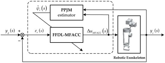
Figure 1.
The block diagram of the FFDL−MFACC scheme.
3.2. Stability Analysis
Theorem 2.
If the robotic exoskeleton (3) is controlled by using the FFDL-MFACC schemes (23)–(25), when
is constrained by condition (11), the following properties can be observed: when the desired signal
,
is a positive number; when , the rehabilitation robot (3) guarantees that (1)
is bounded; (2)
and
are bounded.
Proof.
Theorem 1 is proved in two parts. In part 1, the boundedness of the PPJM estimated matrix is analyzed. For analytical convenience, the estimated error is defined as , . Part 2 proves the boundedness of the tracking error, control input, and system output.
Part 1: By combining (4) and (23) and considering norms and , the following expressions can be obtained:
It should be noted that and , where , , , and . Considering that the robotic system is Lipschitz, there are positive constants , such that , , and thus , . Therefore, , meaning that the following equation holds:
This means that (28) is convergent after s iterations, so we can conclude that and are bounded.
Part 2: Firstly, it is proved that there exists such that:
where is a diagonal matrix, and is the ith diagonal element in the matrix. is the n-dimensional column vector. is a positive number. , are satisfied as follows:
Therefore, the following equation is easily obtained:
denotes the spectral norm, and since ,, , and are all bounded; therefore, the following expressions can be obtained:
Let , ; when , the following equation can be obtained:
Using to denote the spectrum of the matrix, one can obtain the following expression:
According to Theorem 1, when , one obtains the following expression:
This results in a sufficiently small , and a norm , as shown below:
Next, the tracking error is defined as . Using (4), (28), and (29), one can obtain the following equations:
Considering norms on both sides of (38), the following expression can be obtained:
where .
When , . By combining (29) and (39), one obtains the following expressions:
By using (40) and , we can observe that is bounded. From (33), we know that is bounded. Therefore, is bounded; the conclusion (1) of Theorem 2 holds. In addition, is bounded, and the output sequence is also bounded since the reference input signal is bounded. Because the saturation limit is added, the constraint condition is satisfied; it is clear that it is bounded. Thus, conclusion (2) holds. □
Corollary 1.
When holds, the conclusion of Theorem 2 can be strengthened as follows: (1) the system converges in the sequence of tracking errors, namely ; (2) and are bounded.
Proof.
When , we can obtain the following expressions using (38)–(40):
As , one can obtain the following expression using (41):
That is, conclusion (1) of corollary 1 holds. The proof of conclusion (2) in corollary 1 is similar to the proof of conclusion (2) in Theorem 2. □
4. Simulation and Results
In this experiment, the robotic simulation model was built in Simulink using SolidWorks software 2023 SP3 and the SimMechanics toolbox (https://ww2.mathworks.cn/help/sm/gs/simmechanics-first-and-second-generation-comparison.html accessed on 23 July 2022) [35]. The mechanical device has 5-DOF (shoulder, elbow and wrist). To demonstrate the superiority of the proposed FFDL-MFACC scheme, extensive simulation experiments are considered in Examples 1, 2, and 3. In Examples 1 and 2, two control schemes, the adaptive observer-based MFAC scheme [34] and the adaptive sliding mode control (ASMC) scheme [38] are compared with the proposed FFDL-MFACC scheme (23)–(25) in the 3-DOF robot (shoulder and elbow). In Example 3, we perform the 5-DOF robot control according to the FFDL-MFACC scheme (23)–(25).
In this paper, the desired angle velocities [39] are set as , , , ; . We set the simulation time as and sampling period .
4.1. Example 1
To compare the control effect when the actuators are saturated, the execution ability of the actuators is set at , . In Example 1, the desired trajectories of 3-DOF are . The common parameters of the adaptive observer-based MFAC and the FFDL-MFACC are shown in Table 1.

Table 1.
Parameter setting for the adaptive observer-based MFAC and the FFDL-MFACC.
(1) The adaptive observer-based MFAC performance
The estimated PPJM of the adaptive observer-based MFAC scheme is described as follows:
where is the output’s estimated error. is the output’s observed value . is the element on the diagonal of the matrix , , and .
The control input is described as follows:
where the parameters of the adaptive observer-based MFAC scheme are chosen as , , and the other parameters are shown in Table 1. Figure 2 shows the adaptive observer-based MFAC simulation results of 3-DOF.
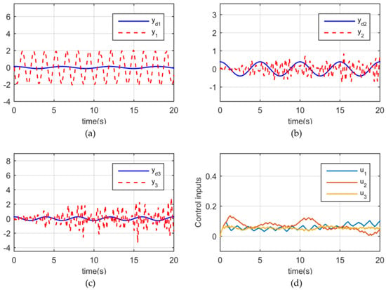
Figure 2.
The adaptive observer−based MFAC simulation results of 3−DOF. (a) Trajectory tracking y1. (b) Trajectory tracking y2. (c) Trajectory tracking y3. (d) Control inputs u1−u3.
(2) The FFDL-MFACC performance
The MFACC scheme is given by (23)–(25). The parameters of the Hildreth quadratic programming method are set as , , , and . The weighting factor is . Figure 3 shows the MFACC simulation results of 3-DOF.
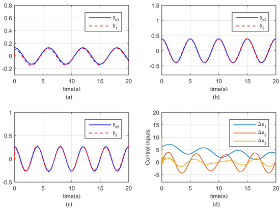
Figure 3.
The FFDL−MFACC simulation results of 3−DOF. (a) Trajectory tracking y1. (b) Trajectory tracking y2. (c) Trajectory tracking y3. (d) Control inputs ∆u1−∆u3.
4.2. Example 2
To verify the robustness of the proposed FFDL-MFACC scheme, an external payload torque was put on the 3-DOF robotic manipulator at the time . The external payload was set as . In Example 2, the desired trajectories of 3-DOF are , and the common parameters of FFDL-MFACC are shown in Table 1. Table 2 shows the performance indexes of the root mean square (RMS) from the ASMC scheme and the FFDL-MFACC scheme in the 3-DOF simulation, respectively.

Table 2.
Performance indexes of the ASMC and the FFDL-MFACC schemes.
(1) The ASMC performance
The adaptive sliding mode control (ASMC) scheme is described as follows:
where , and are unknown parameters for the model. is defined as the sliding surface. denotes the unknown parameter vector, where . The parameters of the ASMC scheme are set as , , and . Let , and Figure 4 shows the ASMC simulation results of 3-DOF.
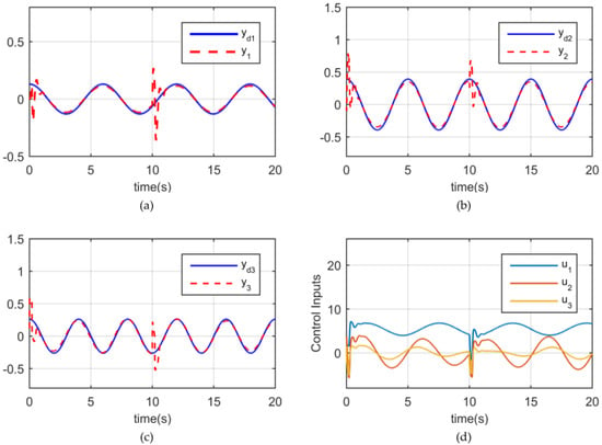
Figure 4.
The ASMC simulation results of 3−DOF. (a) Trajectory tracking y1. (b) Trajectory tracking y2. (c) Trajectory tracking y3. (d) Control inputs u1−u3.
(2) The FFDL-MFACC performance
The MFACC scheme is given by (23)–(25). The parameters of the Hildreth quadratic programming method are set as , , , and . The weighting factor is . Figure 5 shows the MFACC simulation results of 3-DOF.
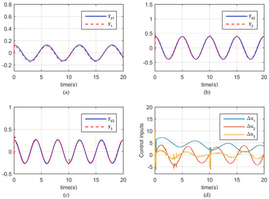
Figure 5.
The FFDL−MFACC with the external payload torque simulation results of 3−DOF. (a) Trajectory tracking y1. (b) Trajectory tracking y2. (c) Trajectory tracking y3. (d) Control inputs ∆u1−∆u3.
Table 2 shows the performance indexes of the root mean square (RMS) from the ASMC scheme and the FFDL-MFACC scheme in the 3-DOF simulation, respectively.
4.3. Example 3
We must consider the controlled joint changes from 3-DOF to 5-DOF and observe the change in trajectories.
(1) The FFDL-MFACC performance
The FFDL-MFACC scheme is given by (23)–(25). The weighting factor is . The parameters of the Hildreth quadratic programming method are set as , , , and . Figure 6 shows the MFACC simulation results of 5-DOF.
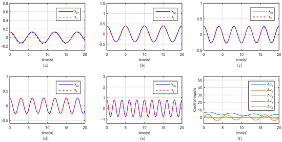
Figure 6.
The FFDL−MFACC simulation results of 5−DOF. (a) Trajectory tracking y1. (b) Trajectory tracking y2. (c) Trajectory tracking y3. (d) Trajectory tracking y4. (e) Trajectory tracking y5. (f) Control inputs ∆u1−∆u5.
4.4. Results Analysis
In Examples 1–3, Figure 2a–c, Figure 3a–c, Figure 4a–c and Figure 5a–c show trajectory tracking of the adaptive observer-based MFAC scheme, the ASMC scheme, and the proposed FFDL-MFAC scheme for the 3-DOF; Figure 6a–e show trajectory tracking for 5-DOF; Figure 2, Figure 3, Figure 4, Figure 5d and Figure 6f show the control signals.
(1) In Example 1, when the actuators are saturated, Figure 2a–c and Figure 3a–c show that the multi-joint tracking performance of the FFDL-MFACC scheme is more stable and fluctuates less than the adaptive observer-based MFAC scheme. In comparative simulation experiments, we find that even with smaller control inputs (see Figure 2d), the adaptive observer-based approach [34] still fails to achieve satisfactory control performance and has more fluctuations in trajectory tracking. It indicates that the FFDL-MFACC method has a good control effect on robot systems with input constraints.
(2) In Example 2, it is clear from Figure 4a–c and Figure 5a–c that the proposed FFDL-MFACC scheme can effectively deal with uncertainties from the external payload torques. Moreover, Table 2 shows that the multi-joint tracking performance of the proposed FFDL-MFACC scheme has more minor dynamic errors than the ASMC scheme. It means that the proposed scheme can handle uncertainties in the robotic exoskeleton system.
(3) In Example 3, when the controlled joint changes from 3-DOF to 5-DOF, it can be seen from Figure 6a–e that the FFDL-MFACC scheme still maintains satisfactory tracking performance. This demonstrates the adaptability of the proposed scheme.
5. Conclusions
This paper presents a data-driven FFDL-MFACC scheme for uncertain rehabilitation exoskeleton robots with input constraints. Firstly, an improved MFAC controller is proposed to address the integral additive effect problem when the existing MFAC method is applied to the robot exoskeleton. The entire controller has a few parameters that need to be adjusted online. Secondly, Hildreth’s quadratic programming procedure method effectively solves the saturated nonlinear problem in the robotic exoskeleton system. Thirdly, the convergence of multi-joint tracking errors and the stability of the bounded input sequence and bounded output sequence of the robotic exoskeleton are proven by the contraction mapping principle. Finally, multiple sets of simulation experiments can be performed on the SimMechanics model to verify the effectiveness of the FFDL-MFACC scheme. In future work, our task will be to plan the practical application of the FFDL-MFACC method in robotic exoskeletons.
Author Contributions
Conceptualization, X.P. and X.F.; methodology, X.P. and L.W.; software, X.P. and L.W.; validation, X.P., X.F. and Y.Z.; formal analysis, X.P. and X.F.; investigation, X.P.; writing—original draft preparation, X.P.; visualization, X.P.; supervision, L.W. and J.W.; project administration, J.W.; funding acquisition, J.W. All authors have read and agreed to the published version of the manuscript.
Funding
This work is supported by the “National Natural Science Foundation of China” (grant 61873054 and 61503070).
Data Availability Statement
Data are contained within the article.
Conflicts of Interest
The authors declare no conflicts of interest.
References
- Sawaki, L. Use-dependent plasticity of the human motor cortex in health and disease. IEEE Eng. Med. Biol. Mag. 2005, 24, 36–39. [Google Scholar] [CrossRef] [PubMed]
- Ito, S.; Kawasaki, H.; Ishigure, Y.; Natsume, M.; Mouri, T.; Nishimoto, Y. A design of fine motion assist equipment for disabled hand in robotic rehabilitation system. J. Frankl. Inst. 2011, 348, 79–89. [Google Scholar] [CrossRef]
- Luijten, F.; Chu, B.; Rogers, E. Iterative learning control for stroke rehabilitation with input dependent muscle fatigue modeling. In Proceedings of the 2018 Annual American Control Conference, Milwaukee, WI, USA, 27–29 June 2018; pp. 6396–6401. [Google Scholar]
- Kang, H.B.; Wang, J.H. Adaptive robust control of 5 DOF Upper-limb exoskeleton robot. Int. J. Control Autom. Syst. 2015, 13, 733–741. [Google Scholar] [CrossRef]
- Hogan, N.; Krebs, H.I.; Charnnarong, J.; Srikrishna, P.; Sharon, A. MIT-MANUS: A workstation for manual therapy and training. I. In Proceedings of the Proceedings IEEE International Workshop on Robot and Human Communication, Nice, France, 12–14 May 1992; pp. 161–165. [Google Scholar]
- Lum, P.S.; Burgar, C.G.; Van der Loos, M.; Shor, P.C.; Majmundar, M.; Yap, R. The MIME robotic system for upper-limb neuro-rehabilitation: Results from a clinical trial in subacute stroke. In Proceedings of the 9th International Conference on Rehabilitation Robotics, Chicago, IL, USA, 28 June–1 July 2005; pp. 511–514. [Google Scholar]
- Nef, T.; Mihelj, M.; Riener, R. ARMin: A robot for patient-cooperative arm therapy. Med. Biol. Eng. Comput. 2007, 45, 887–900. [Google Scholar] [CrossRef]
- Fazekas, G.; Horvath, M.; Toth, A. A novel robot training system designed to supplement upper limb physiotherapy of patients with spastic hemiparesis. Int. J. Rehabil. Res. 2006, 29, 251–254. [Google Scholar] [CrossRef]
- Perry, J.C.; Rosen, J.; Burns, S. Upper-limb powered exoskeleton design. IEEE/ASME Trans. Mechatron. 2007, 12, 408–417. [Google Scholar] [CrossRef]
- Mao, Y.; Agrawal, S.K. Design of a cable-driven arm exoskeleton (CAREX) for neural rehabilitation. IEEE Trans. Robot. 2012, 28, 922–931. [Google Scholar] [CrossRef]
- Lee, M.; Rittenhouse, M.; Abdullah, H.A. Design issues for therapeutic robot systems: Results from a survey of physiotherapists. J. Intell. Robot. Syst. 2005, 42, 239–252. [Google Scholar] [CrossRef]
- Proietti, T.; Crocher, V.; Roby-Brami, A.; Jarrasse, N. Upper-limb robotic exoskeletons for neurorehabilitation: A review on control strategies. IEEE Rev. Biomed. Eng. 2016, 9, 4–14. [Google Scholar] [CrossRef]
- Li, Z.; Huang, Z.; He, W.; Su, C.Y. Adaptive impedance control for an upper limb robotic exoskeleton using biological signals. IEEE Trans. Ind. Electron. 2016, 64, 1664–1674. [Google Scholar] [CrossRef]
- Chen, Z.; Li, Z.; Chen, C.P. Disturbance observer-based fuzzy control of uncertain MIMO mechanical systems with input nonlinearities and its application to robotic exoskeleton. IEEE Trans. Cybern. 2016, 47, 984–994. [Google Scholar] [CrossRef] [PubMed]
- Yang, Z.; Peng, J.; Liu, Y. Adaptive neural network force tracking impedance control for uncertain robotic manipulator based on nonlinear velocity observer. Neurocomputing 2019, 331, 263–280. [Google Scholar] [CrossRef]
- Li, Z.; Liu, J.; Huang, Z.; Peng, Y.; Pu, H.; Ding, L. Adaptive impedance control of human–robot cooperation using reinforcement learning. IEEE Trans. Ind. Electron. 2017, 64, 8013–8022. [Google Scholar] [CrossRef]
- Yu, X.; He, W.; Li, Y.; Xue, C.; Li, J.; Zou, J.; Yang, C. Bayesian estimation of human impedance and motion intention for human–robot collaboration. IEEE Trans. Cybern. 2019, 51, 1822–1834. [Google Scholar] [CrossRef]
- Yu, X.; He, W.; Li, H.; Sun, J. Adaptive fuzzy full-state and output-feedback control for uncertain robots with output constraint. IEEE Trans. Syst. Man Cybern. Syst. 2020, 51, 6994–7007. [Google Scholar] [CrossRef]
- Yin, S.; Ding, S.X.; Xie, X.; Luo, H. A review on basic data-driven approaches for industrial process monitoring. IEEE Trans. Ind. Electron. 2014, 61, 6418–6428. [Google Scholar] [CrossRef]
- Yin, S.; Li, X.; Gao, H.; Kaynak, O. Data-based techniques focused on modern industry: An overview. IEEE Trans. Ind. Electron. 2014, 62, 657–667. [Google Scholar] [CrossRef]
- Hou, Z.S.; Wang, Z. From model-based control to data-driven control: Survey, classification and perspective. Inf. Sci. 2013, 235, 3–5. [Google Scholar] [CrossRef]
- Astrom, K.J.; Hagglund, T. PID Controllers: Theory, Design and Tuning, 2nd ed.; The International Society of Measurement and Control: Research Triangle Park, NC, USA, 1995. [Google Scholar]
- Hjalmarsson, H.; Gevers, M.; Gunnarsson, S.; Lequin, O. Iterative feedback tuning: Theory and applications. IEEE Control Syst. Mag. 1998, 18, 26–41. [Google Scholar]
- Campi, M.C.; Lecchini, A.; Savaresi, S.M. Virtual reference feedback tuning: A direct method for the design of feedback controllers. Automatica 2002, 38, 1337–1346. [Google Scholar] [CrossRef]
- Hou, Z.; Jin, S. Model Free Adaptive Control: Theory and Applications; CRC Press: Boca Raton, FL, USA, 2013. [Google Scholar]
- Hou, Z.; Xiong, S. On model-free adaptive control and its stability analysis. IEEE Trans. Autom. Control 2019, 64, 4555–4569. [Google Scholar] [CrossRef]
- Wang, Y.; Wang, Z. Model-free adaptive tracking control for networked nonlinear systems with data dropout. Int. J. Robust Nonlinear Control 2022, 32, 1453–1468. [Google Scholar] [CrossRef]
- Liu, D.; Liu, N.; Li, T. Event-triggered model-free adaptive control for nonlinear systems with output saturation. Int. J. Robust Nonlinear Control 2023, 33, 7204–7220. [Google Scholar] [CrossRef]
- Hou, Z.; Bu, X. Model-free adaptive control with data dropouts. Expert Syst. Appl. 2011, 38, 10709–10717. [Google Scholar] [CrossRef]
- Hou, Z.; Jin, S. Data-driven model-free adaptive control for a class of MIMO nonlinear discrete-time systems. IEEE Trans. Neural Netw. 2011, 22, 2173–2188. [Google Scholar] [PubMed]
- Zhu, Y.; Hou, Z. Controller dynamic linearisation-based model-free adaptive control framework for a class of non-linear system. IET Control Theory Appl. 2015, 9, 1162–1172. [Google Scholar] [CrossRef]
- Liu, T.; Hou, Z. Model-free adaptive containment control for unknown multi-input multi-output nonlinear MASs with output saturation. IEEE Trans. Circuits Syst. I Regul. Pap. 2023, 70, 2156–2166. [Google Scholar] [CrossRef]
- Bu, X.; Liang, J.; Hou, Z.; Chi, R. Data-driven terminal iterative learning consensus for nonlinear multiagent systems with output saturation. IEEE Trans. Neural Netw. Learn. Syst. 2020, 32, 1963–1973. [Google Scholar] [CrossRef]
- Xu, D.; Jiang, B.; Shi, P. A novel model-free adaptive control design for multivariable industrial processes. IEEE Trans. Ind. Electron. 2014, 61, 6391–6398. [Google Scholar] [CrossRef]
- Wang, X.; Li, X.; Wang, J.; Fang, X.; Zhu, X. Data-driven model-free adaptive sliding mode control for the multi degree-of-freedom robotic exoskeleton. Inf. Sci. 2016, 327, 246–257. [Google Scholar] [CrossRef]
- Yang, H.; Gao, X.; Chen, Y.; Hao, L. Hammerstein adaptive impedance controller for bionic wrist joint actuated by pneumatic muscles. IEEE Access 2018, 7, 47–56. [Google Scholar] [CrossRef]
- Wang, L. Model Predictive Control System Design and Implementation Using Matlab; Springer: Berlin/Heidelberg, Germany, 2009. [Google Scholar]
- Slotine, J.J.; Li, W. On the adaptive control of robot manipulators. Int. J. Robot. Res. 1987, 6, 49–59. [Google Scholar] [CrossRef]
- Głowiński, S.; Krzyżyński, T.; Pecolt, S.; Maciejewski, I. Design of motion trajectory of an arm exoskeleton. Arch. Appl. Mech. 2015, 85, 75–87. [Google Scholar] [CrossRef]
Disclaimer/Publisher’s Note: The statements, opinions and data contained in all publications are solely those of the individual author(s) and contributor(s) and not of MDPI and/or the editor(s). MDPI and/or the editor(s) disclaim responsibility for any injury to people or property resulting from any ideas, methods, instructions or products referred to in the content. |
© 2024 by the authors. Licensee MDPI, Basel, Switzerland. This article is an open access article distributed under the terms and conditions of the Creative Commons Attribution (CC BY) license (https://creativecommons.org/licenses/by/4.0/).