A Soft Sensor Model for Predicting the Flow of a Hydraulic Pump Based on Graph Convolutional Network–Long Short-Term Memory

Abstract

The hydraulic pump plays a pivotal role in engineering machinery, and it is essential to continuously monitor its operating status. However, many vital signals for monitoring cannot be directly obtained in practical applications. To address this, we propose a soft sensor approach for predicting the flow signal of the hydraulic pump based on a graph convolutional network (GCN) and long short-term memory (LSTM). Our innovative GCN-LSTM model is intricately designed to capture both spatial and temporal interdependencies inherent in complex machinery, such as hydraulic pumps. We used the GCN to extract spatial features and LSTM to extract temporal features of the process variables. To evaluate the performance of GCN-LSTM in predicting the flow of a hydraulic pump, we construct a real-world experimental dataset with an actual hydraulic shovel. We further evaluated GCN-LSTM on two public datasets, showing the effectiveness of GCN-LSTM for predicting the flow of hydraulic pumps and other complex engineering operations.

1. Introduction

The hydraulic pump is a crucial power component that is widely used in modern industrial equipment, including mining and metallurgy, national defense construction, power systems, agricultural machinery, chemicals and petroleum, and shipbuilding [1,2,3]. The performance of a hydraulic pump directly affects the operational efficiency and accuracy of the powered mechanical equipment. Therefore, continuous monitoring of the operating status of the hydraulic pump is of significant practical importance and can help operators detect and solve hydraulic pump failures in a timely manner, ensuring the safe operation of the equipment [4,5,6]. However, in many real-world engineering applications, real-time monitoring through direct sensing is often impractical due to factors such as harsh working environments, the prohibitive cost of monitoring equipment, and difficulty in sensor installation. Additionally, the complex and nonlinear features of the operating process present challenges for equipment process monitoring, fault diagnosis, and health assessment [7]. To address these issues, soft sensor technology has been proposed. It estimates or predicts the conditions of a physical system based on other process variables that can be easily measured [8,9]. A basic soft sensor framework includes auxiliary variable selection, data acquisition, establishment of soft sensor models, and subsequent online model application [10].

Generally, soft sensing technology encompasses two main types of methods: mechanism-based models and data-driven models. Mechanism-based methods offer good interpretability and can explain the interrelationships between systems and components [11]. However, mechanism models inevitably introduce modeling errors due to the dynamic nature of the production process, affecting measurement accuracy and limiting practical operations [12]. Data-driven methods do not require extensive prior knowledge and can establish accurate soft measurement models by acquiring multiple data information from the equipment through sensor installation, provided relatively complete data are ensured. Data-driven soft measurement methods have gained popularity due to their better adaptability and accuracy compared to mechanism models. These methods mainly fall into two categories: traditional machine learning models and deep learning models [13]. Traditional data-driven methods are based on statistical inference [14], regression analysis [15], and machine learning [16], including principal component analysis (PCA) [17], partial least squares (PLS) [18], support vector machines (SVMs) [19], artificial neural networks (ANNs) [20], and principal component regression (PCR) [21]. They are widely used for linear and steady-state system modeling. However, these machine learning models have proven inadequate for accurate soft sensing in complex industrial processes [22]. To more effectively simulate complex industrial processes and extract nonlinear and dynamic information from data, data-driven models based on deep learning have been developed. Deep learning models possess powerful learning and nonlinear fitting capabilities [23], enabling them to generate deep and abstract feature representations. They have been extensively researched and applied in industrial applications [24]. Various deep learning models, such as autoencoders (AEs) [25], restricted Boltzmann machines (RBMs) [26], and convolutional neural networks (CNNs) [27], as well as recurrent neural networks (RNNs) [28] and long short-term memory networks (LSTMs) [29], have been successfully applied to soft sensor development, achieving promising prediction results. There have been numerous research achievements in soft sensor technology based on deep learning, such as, such as, Sun et al. proposed a deep feature extraction and layer-by-layer integration method based on a gated stack target correlation autoencoder (GSTAE) for industrial soft sensing applications [30]. To solve the problem of high nonlinearity and strong correlation between multiple variables in the process of a coal-fired boiler, a deep structure using continuous RBM and SVR algorithms is proposed [31]. Yuan et al. proposed a multichannel CNN for soft sensing applications in industrial fractionation columns and hydrocracking processes, which can learn the dynamics and various local correlations of different variable combinations [32]. To extract temporal features, an RNN was introduced to construct a nonlinear dynamic soft sensor model for the batch process [33,34].

In practical industrial processes, soft sensor modeling often involves process variables characterized as non-Euclidean structured graph data, exhibiting intricate spatial coupling relationships that influence variable variations throughout complex operating processes [35]. In addition to capturing their temporal relationships, it is also critical to effectively capture the potential spatial coupling relationships between the process variables. Recent studies have introduced graph neural network (GNN) or graph convolutional network (GCN) technology to explicitly represent the spatial coupling relationships between process variables [36,37]. For example, Wang et al. utilized a GCN to capture the spatial features of the power grid for voltage stability prediction [38]. Ta et al. proposed an adaptive spatiotemporal graph neural network to capture the spatiotemporal correlations of vehicles for traffic flow prediction [39]. Yu et al. combined a GCN and a CNN to, respectively, extract the temporal and spatial correlations of traffic conditions [40]. Wang et al. proposed an adaptive multichannel graph convolutional network (AM-GCN) for semi-supervised classification, extracting specific and common embeddings from node features, topological structures, and their combinations. Attention mechanisms were employed to learn the adaptive importance weight of embeddings [41]. Zhou et al. constructed a dynamic graph data processing framework for rotating machinery diagnosis [42]. Multi et al. introduced an improved multichannel graph convolutional network for rotating machinery diagnosis to learn graph features and achieve multichannel feature fusion [43].

In the field of engineering machinery, most existing soft sensor studies are based on limited experimental data obtained from test benches or simulations for performance evaluation [44]. To better evaluate the effectiveness of our proposed GCN-LSTM as a soft sensor model for predicting hydraulic pump flow, we constructed a real-world experimental dataset using actual operational data from a hydraulic shovel under various operating conditions. We further evaluated GCN-LSTM on two public datasets, demonstrating its effectiveness for predicting hydraulic pump flow in practical settings and other complex engineering operations.

The main contents in this paper are as follows:

(1)

We proposed a novel soft sensor model for predicting the flow of hydraulic pumps by combining a GCN and LSTM. We used a GCN to capture the spatial features of the process variable and LSTM to capture their temporal features;

(2)

We collected a first-of-its-kind real-world dataset of a hydraulic shovel with actual operational conditions and showed that our proposed GCN-LSTM model was also able to outperform current deep learning approaches for predicting the flow of hydraulic pumps in practical settings;

(3)

We validated the proposed GCN-LSTM model on two public datasets and showed that our GCN-LSTM model outperformed current deep learning approaches for other complex engineering operations.

2. Methods

2.1. Principles of GCN

A graph convolutional neural network (GCN) is a type of convolutional neural network (CNN) that focuses on modeling graph data [45,46]. It utilizes graph convolution to extract the spatial features of non-Euclidean structured graph data. GCNs have been developed based on the theory proposed in [47], which suggests that they are more suitable for handling non-Euclidean structured data compared to traditional CNNs.

Figure 1 depicts the network diagram of a GCN. The GCN has multiple hidden layers with the following activation function:

$$\mathrm{Re}\mathrm{LU}(x)=\max \{0,x\}$$

(1)

The input data for a GCN consists of two essential components: node feature data and graph structural information. The graph structural information can be represented by an adjacency matrix, typically denoted as A. The adjacency matrix A_ij captures the connectivity between nodes in the underlying graph G, where G comprises a set of nodes V (v_i, v_j ∈ V). The entries in the adjacency matrix A_ij indicate the connectivity between nodes v_i and v_j in the graph. The function expressions for the input signal M and output signal Y are as follows:

$$f(M,A)=Y$$

(2)

The specific calculations of the GCN in the hidden layer are defined as:

$$H^{(l+1)}=relu({\tilde{D}}^{-\frac{1}{2}}\tilde{A}{\tilde{D}}^{-\frac{1}{2}}{H}^{(l)}{W}^{(l)}$$

(3)

$${\tilde{D}}_{ii}={\displaystyle \sum _j{\tilde{A}}_{ij}}$$

(4)

$$\tilde{A}=A+I$$

(5)

H represents the calculation result of the GCN network in the hidden layer, where the initial value H⁽⁰⁾ of H is set to the input data M, and W^(l) represents the weight matrix in (3). $\tilde{D}$ is a diagonal matrix in Equation (4), and I represents the identity matrix of the same order as the adjacency matrix A in Equation (5).

2.2. Principles of LSTM

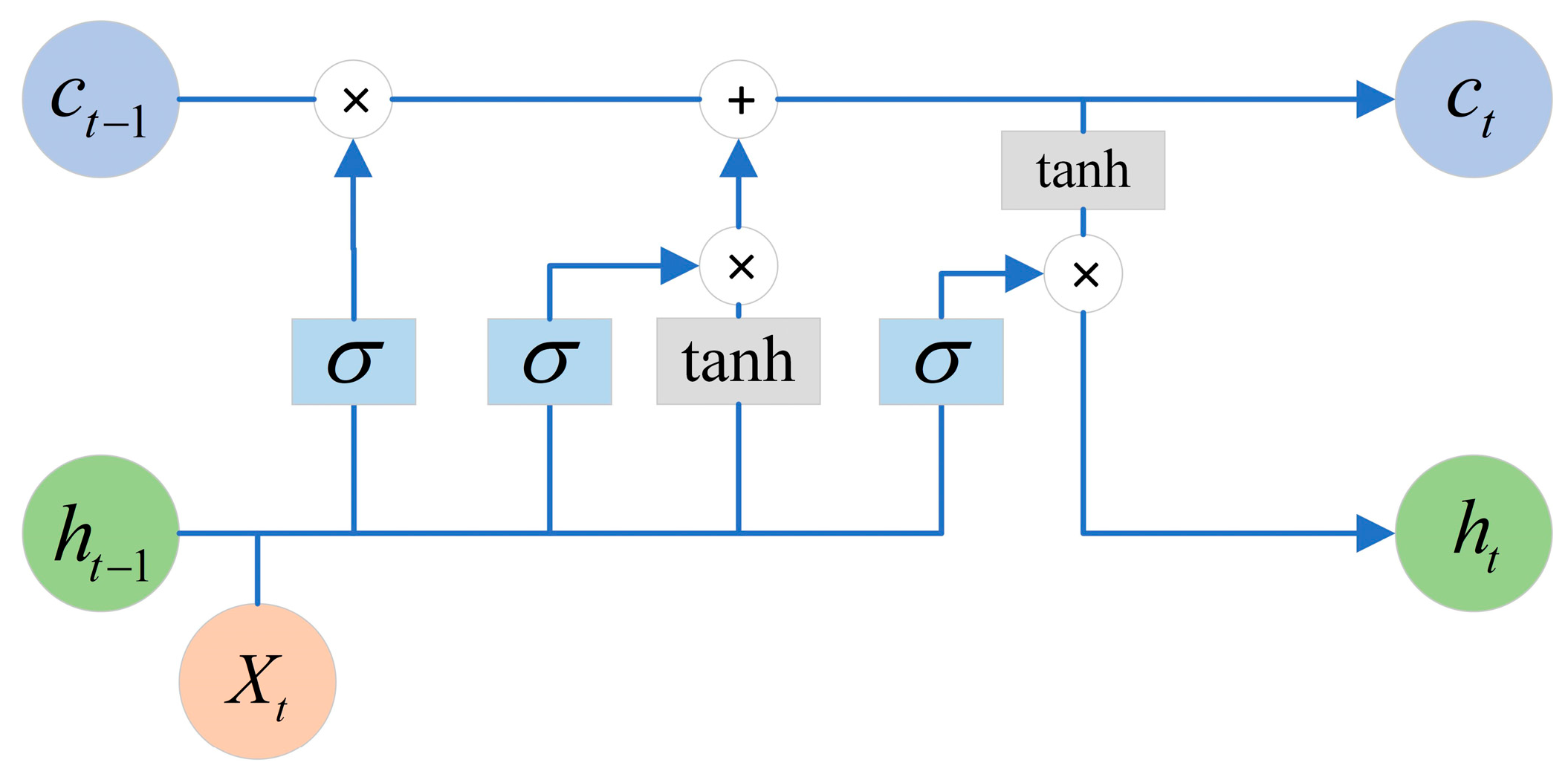
Long short-term memory networks (LSTMs), proposed by Hochreiter and Schmidhuber (1997) [48], consist of three key components: a forget gate, input gate, and output gate. The LSTM network structure is shown in Figure 2.

The first step of LSTM is to decide which information to discard from the cell state, as shown in Equation (6) below:

$$f_t=\sigma ([h_{t-1},x_t]{\displaystyle •}{W}_f+b_f)$$

(6)

where f_t is the scale factor controlling the forgotten information at the current moment; $\sigma$ is the sigmoid activation function mapping the calculated data smoothly to the interval (0, 1), which corresponds exactly to the switching degree of the control gate; W_f is the weight matrix of the forget gate; and b_f is the bias term of the forgot gate.

Next, the input gate determines what new information is stored in the cell state c_t, as shown in Equations (7) and (8) below:

$$i_t=\sigma ([h_{t-1},x_t]•W_i+b_i)$$

(7)

$${\tilde{c}}_t=\tanh ([h_{t-1},x_t]•W_c+b_c)$$

(8)

where i_t is the scale factor of the control input information at the current moment; ${\tilde{c}}_t$ is the candidate cell state at the current moment; tanh is the activation function; W_c is the weight matrix of the candidate cell state; and b_c is the bias term of the candidate cell state.

LSTM then proceeds to multiply the old state by f_t to discard the information that needs to be forgotten, and then we add $i_t\ast {\tilde{c}}_t$ to obtain the new candidate value, which changes according to the degree of updating each state, as shown in Equation (9) below:

$$c_t=f_t\ast c_{t-1}+i_t\ast {\tilde{c}}_t$$

(9)

Finally, the output gate determines what value needs to be output by LSTM, as shown in Equations (10) and (11) below:

$$o_t=\sigma ([h_{t-1},x_t]•W_o+b_o)$$

(10)

$$h_t=o_t\ast \tanh (c_t)$$

(11)

2.3. GCN-LSTM Model

The prediction problem of the target variable can be defined as follows: predicting the target value at the next time step using the historical time series data and considering a monitoring duration and the spatial relationship between each variable. In the case of flow prediction for a hydraulic pump, a sliding window approach is employed to select multiple sets of relevant variable signals for prediction. The duration for which the variables are selected is denoted as t, the spatial relationship between each sensor is represented as A, and the model predicts the flow value y at time t + 1, as shown in Equation (12):

$$y_{t+1}=F({[M_1,M_2,\dots ,M_k]}_t;A)$$

(12)

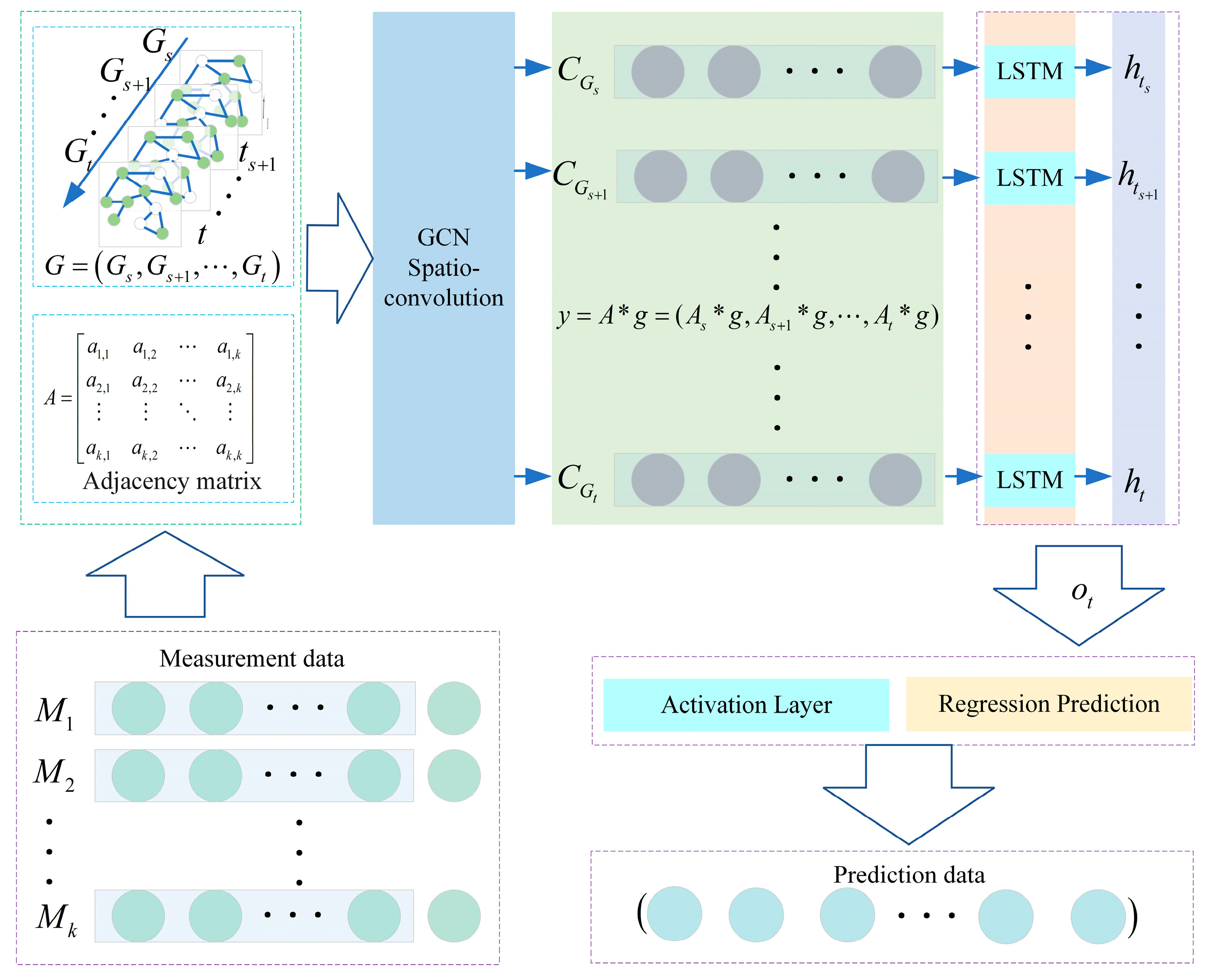
In other words, the prediction of the flow value $y$ (target variable) at the next time step is computed using the historical time series data within a monitoring duration based on the spatial relationship between each variable. In Equation (12), y_t+1 represents the predicted flow of the hydraulic pump at time t + 1 using F, which represents the soft sensor model based on our proposed GCN-LSTM model, as shown in Figure 3. A represents the spatial relationship between different sensors as an adjacency matrix, as shown in Equations (13) and (15).

$$A=\left[\begin{array}{ccc}{a}_{1,1}& \cdots & a_{1,k}\\ ⋮& \ddots & ⋮\\ a_{k,1}& \cdots & a_{k,k}\end{array}\right]\in R^{k\times k}$$

(13)

$$\mathrm{where}{a}_{k1},a_{k2}=\left\{\begin{array}{l}1,k_1\leftrightarrow k_2\\ 0,others\end{array}\right.$$

(14)

In our GCN-LSTM model, the GCN extracts spatial feature information of variables through spatioconvolution operations, outputting the structural information in the graph and the features of the nodes to form new feature vectors for each node, i.e., C_G = (C_Gs, C_Gs, …, C_Gt), as the input to LSTM to capture the temporal features. *g is a convolutional operation based on the GCN. Then, the output of LSTM serves as the input to the activation layer for regression prediction, and thus the target variable sequence is generated.

The GCN-LSTM model adopts a sliding prediction approach [49]. In this work, we use sliding window size SW = 30 to predict the target values. During the training process, a regression model is trained using the minimization of prediction errors. The training and testing process of the GCN-LSTM model is shown in Figure 4.

To assess the effectiveness of the soft sensor model, the root-mean-square error (RMSE) and the coefficient of determination R² [50] are commonly used. They are defined as follows:

$$RMSE=\sqrt{\frac{1}{N_{test}}{\displaystyle \sum _{i=1}^{N_{test}}{({\widehat{y}}_i-y_i)}^2}}$$

(15)

$$R^2=1-\frac{{\displaystyle {\sum }_{i=1}^{N_{test}}{({\widehat{y}}_i-y_i)}^2}}{{\displaystyle {\sum }_{i=1}^{N_{test}}{(y_i-\overline{y})}^2}}$$

(16)

3. Case Studies: Hydraulic Pump

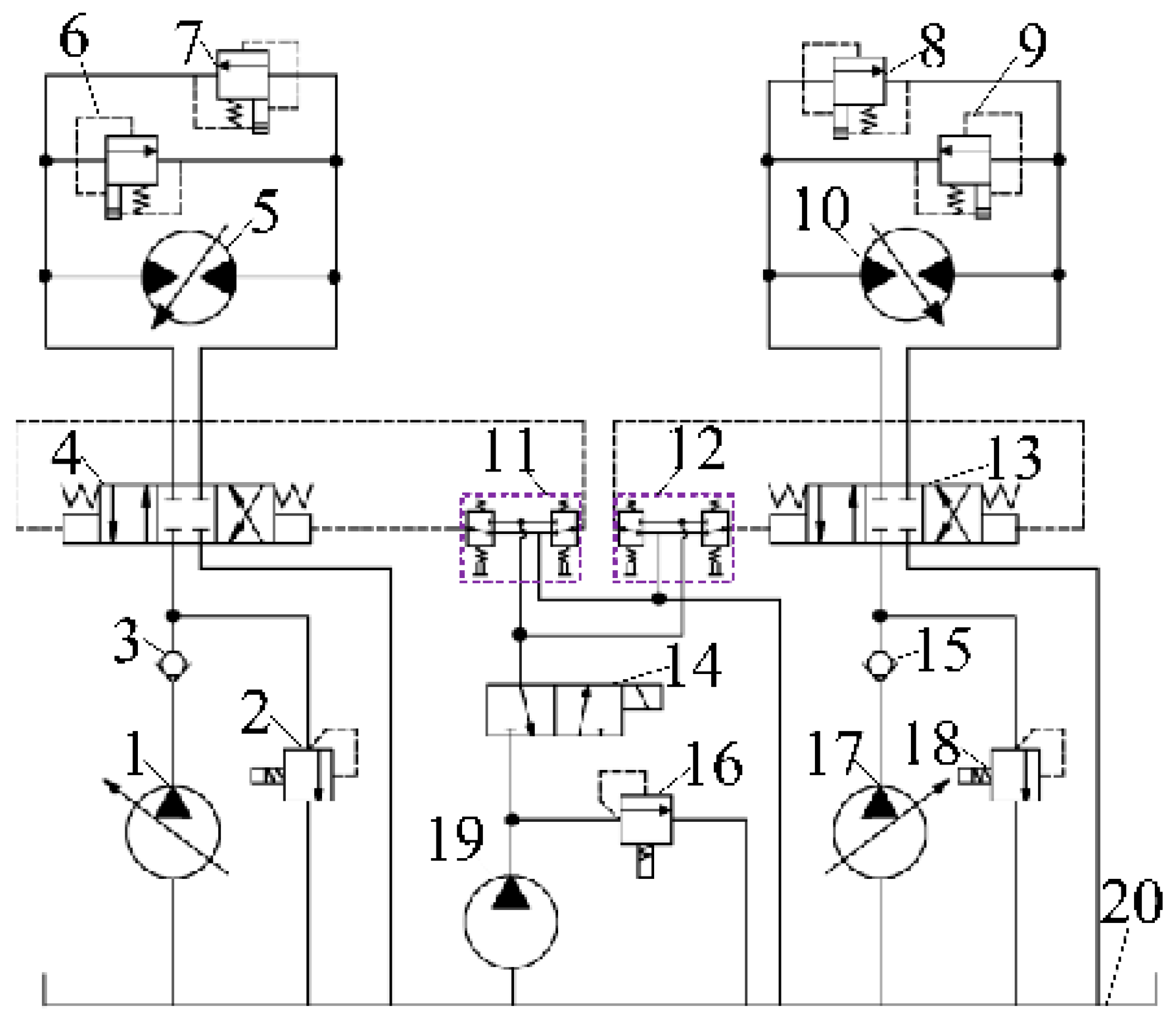
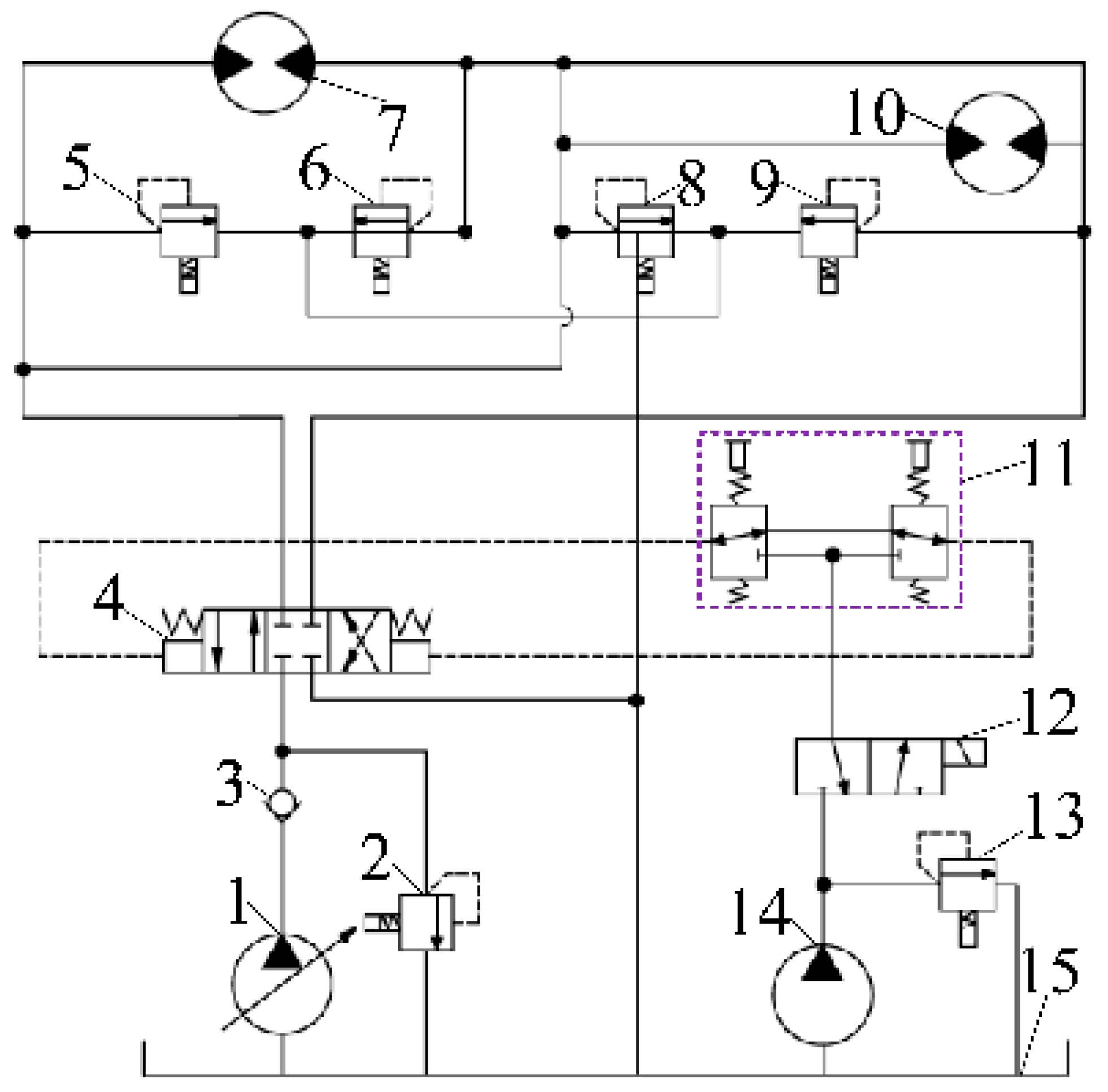
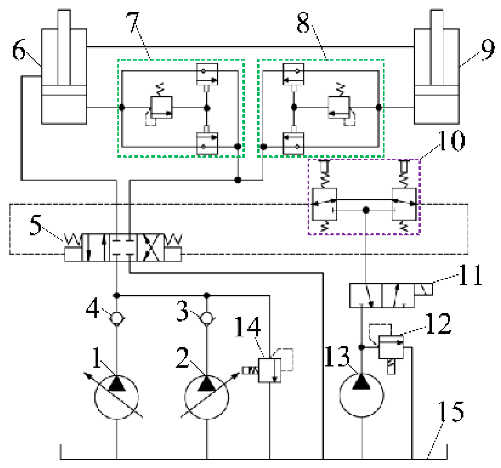
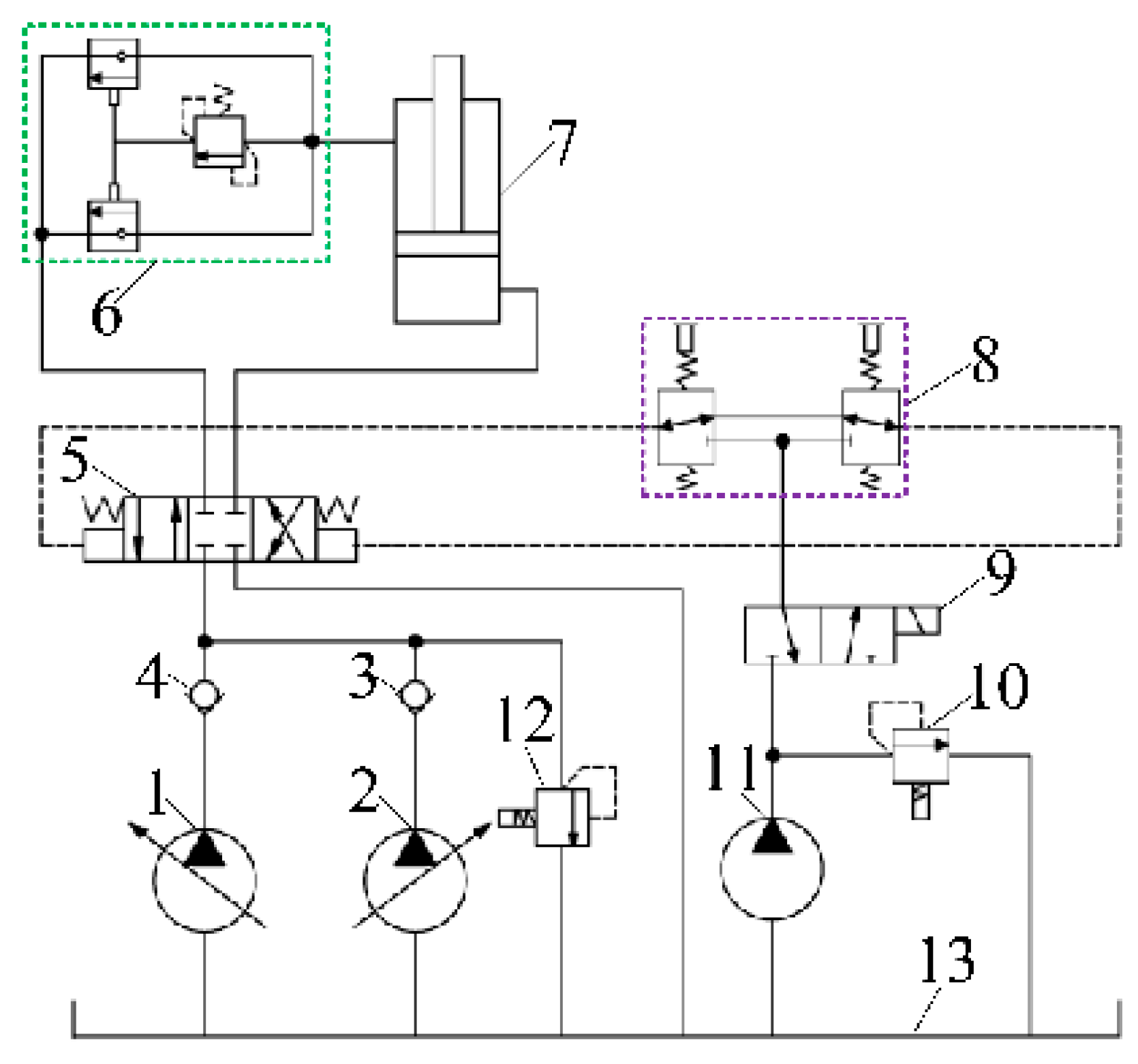
Given that most existing soft sensor studies are largely based on limited experimental data obtained from test benches or simulation simulations for performance evaluation [20], we construct a real-world experimental dataset with actual hydraulic shovel operating data under multiple different operating conditions to better evaluate the effectiveness of our proposed GCN-LSTM model as a soft sensor model for predicting the flow of a hydraulic pump. To collect the real-world dataset, we designed an operational condition experiment for an XCMG hydraulic shovel and considered the three operational conditions: swing action, walking action, and digging composite action (boom, arm, and bucket) of the hydraulic shovel for predicting pump flow. The hydraulic system diagrams for each action are shown in Figure 5, Figure 6, Figure 7, Figure 8 and Figure 9. In the hydraulic system of a hydraulic excavator, there are two hydraulic pumps as power sources, namely pump 1 and pump 2. Among them, during the swing motion, only pump 2 serves as the power source, while during the walking and digging composite actions, both pump 1 and pump 2 serve as power sources.

For performance analysis, two baseline methods are compared with GCN-LSTM: supervised LSTM (S-LSTM) [51] and variable attention-based long short-term memory (VA-LSTM) [52], which are the soft sensor models. These methods were all developed based on the PyTorch architecture. In the training process of the model, the Adam optimizer was used to train the network parameters. These models run on a Windows 10 system and a server equipped with an Intel i7-9700 3.00 GHz CPU, an NVIDIA GeForce GTX 1050 Ti, and 16 GB memory.

3.1. Experimental Setup

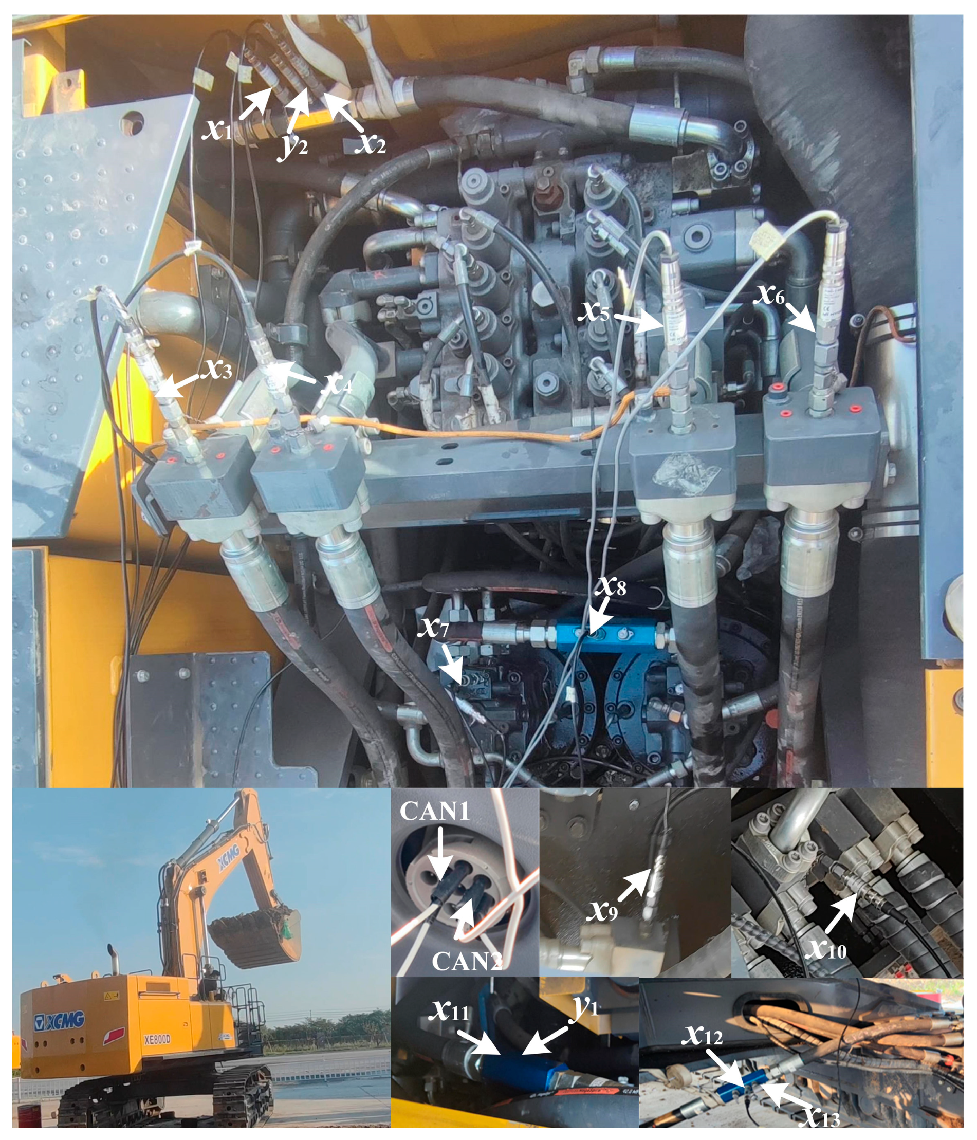
This experiment involves two data acquisition paths: onboard data obtained through the CAN bus and external sensors. The onboard data include two parts: CAN1 and CAN2. CAN1 captures signals, such as pump pressure and pilot pressure, while CAN2 collects signals, such as engine speed and engine torque percentage. By analyzing the onboard data, we determined that the sampling frequency of CAN1 is 5 Hz, and the sampling frequency of CAN2 is 20 Hz. Our primary focus was on data collection through external sensors. For this purpose, we employed two eight-channel USB3100N acquisition cards capable of a maximum sampling rate of 2.5 kHz. Considering the sampling rates of the onboard CAN1 and CAN2, along with Figure 5, Figure 6, Figure 7, Figure 8 and Figure 9, we set the sampling rate of these sensors at 200 Hz.

Table 1. Hydraulic shovel variables collected based on swing, walking, and composite actions.

Variables	Description
x1	Pump 2 oil temperature
x2	Pump 2 pressure
x3	Bucket small chamber pressure
x4	Bucket large chamber pressure
x5	Boom large chamber pressure
x6	Boom small chamber pressure
x7	Swing motor pressure
x8	Swing motor flow
x9	Arm large chamber pressure
x10	Arm small chamber pressure
x11	Pump 1 pressure
x12	Walking motor flow
x13	Walking motor pressure
x14	Swing pilot pressure
x15	Left walking pilot pressure
x16	Right walking pilot pressure
x17	Arm inward pilot pressure
x18	Arm outward pilot pressure
x19	Boom inward pilot pressure
x20	Boom outward pilot pressure
x21	Bucket inward pilot pressure
x22	Bucket outward pilot pressure
x23	Engine speed
x24	Engine torque percentage
y1	Pump 1 flow
y2	Pump 2 flow

shows the list of the collected variables. The objective of GCN-LSTM is to predict the flow of pump 1 and pump 2 based on the swing action condition, walking action condition, and excavation composite action condition of the hydraulic shovel.

The sensors and acquisition equipment for data collection are shown in Figure 10. GCN-LSTM hyperparameters are set based on the prediction process, as shown in

Table 2. Main hyperparameters of the GCN-LSTM model.

Name	Main Parameters
LSTM	n = 50, dropout = 0.2
LSTM	n = 50, dropout = 0.2
Dense	1
Dropout	0.2
Epochs	200
Batch size	30

.

3.2. Pump Flow Prediction under Swing Action

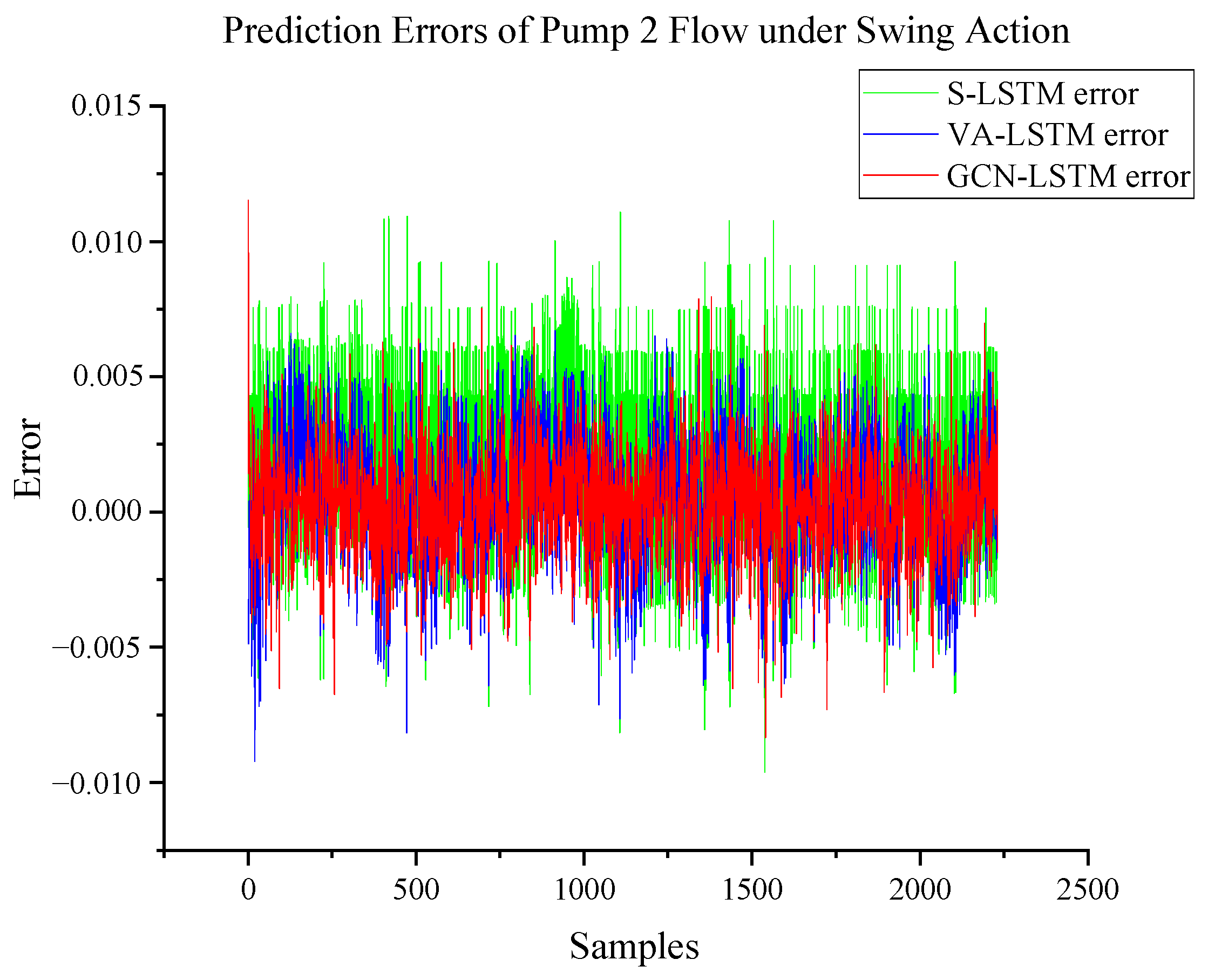
Based on the analysis of the hydraulic shovel swing operation mechanism, it is determined that only pump 2 provides flow, making it the target variable (y₂). Referring to Table 1, the variables associated with the swing action are x₁, x₂, x₇, x₈, x₂₃, and x₂₄. Figure 11 and Figure 12 depict the prediction and errors of pump 2 flow using the GCN-LSTM, S-LSTM, and VA-LSTM models on the testing dataset. The predicted errors for all three models mostly fall within the range of [−0.010, 0.010]. This is because the prediction is based on data collected under steady-state conditions with constant speed rotation. As a result, all three methods have good prediction accuracy. Notably, the prediction curves generated by the GCN-LSTM model closely align with the actual output curves in the testing dataset. This indicates that the GCN-LSTM model has the ability to accurately track the real output and perform well in predicting pump 2 flow.

3.3. Pump Flow Prediction under Walking Action

Based on the analysis of the hydraulic shovel walking operation mechanism, it is determined that both pump 1 and pump 2 provide equal flow. Therefore, we will focus solely on predicting the flow of pump 1, making it the target (y₁). Referring to Table 1, the variables associated with the walking action are x₁₁, x₁₂, x₁₃, x₁₅, x₁₆, x₂₃, and x₂₄.

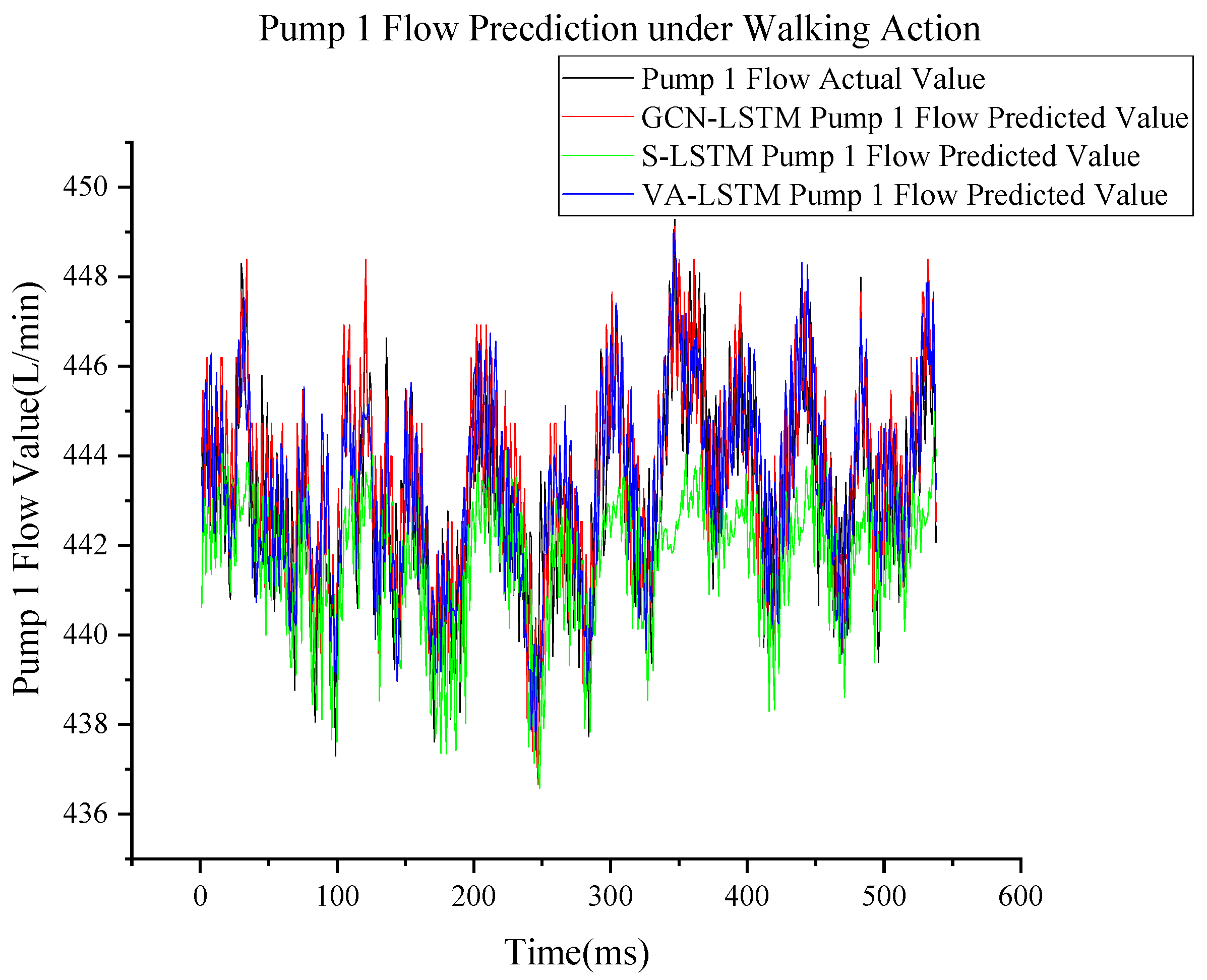
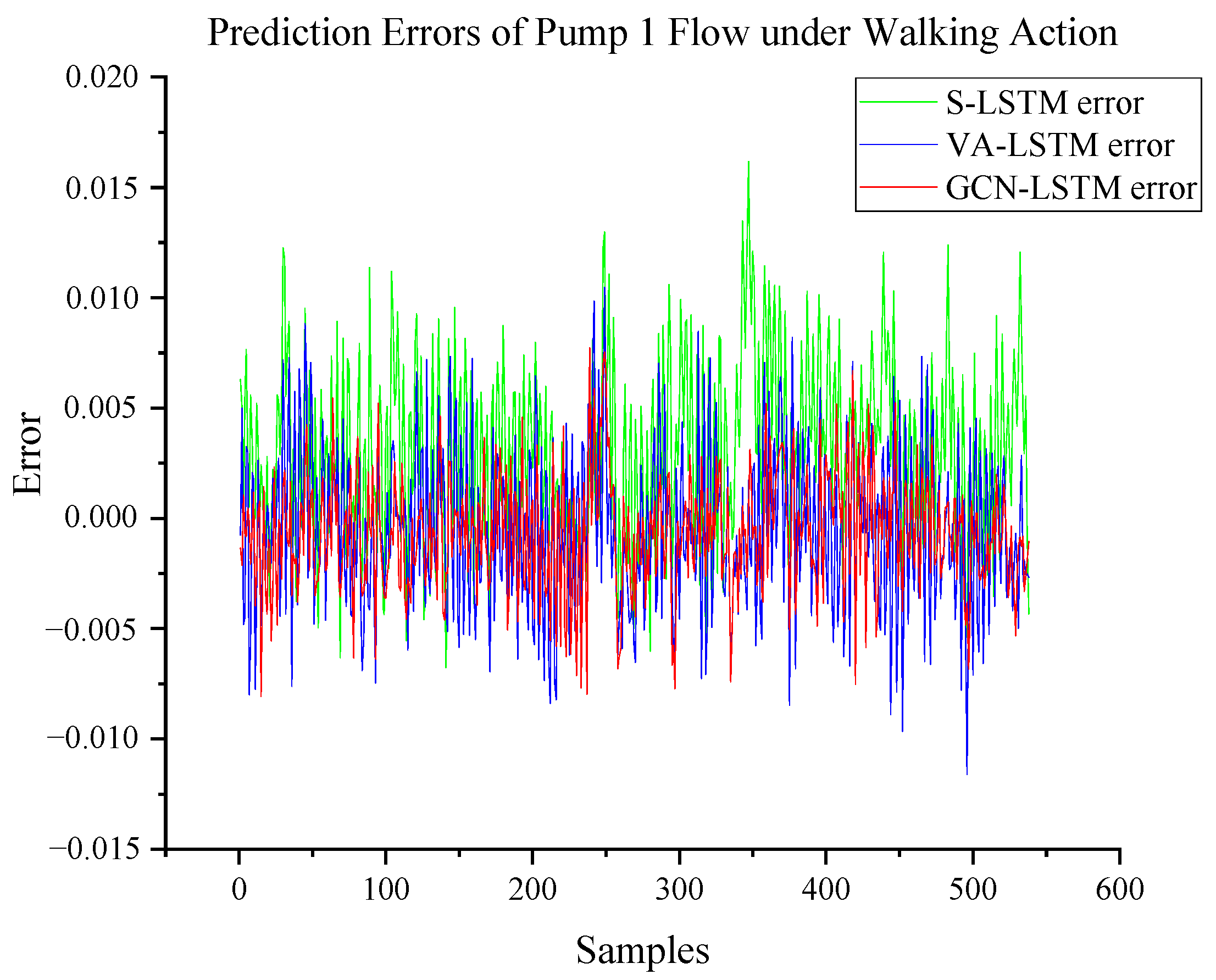
Figure 13 and Figure 14 depict the prediction and errors of pump 1 flow using the GCN-LSTM, S-LSTM, and VA-LSTM models on the testing dataset, respectively. Notably, all three models demonstrate the ability to closely track the actual output curves in the testing dataset. The predicted errors for the three models mostly fall within the range of [−0.015, 0.020], indicating that they have relatively small errors. Among the three methods, our proposed GCN-LSTM model exhibits the smallest error, suggesting its superior performance in predicting pump 1 flow.

3.4. Pump Flow Prediction under Composite Action

Based on the analysis of the hydraulic shovel composite operation mechanism, the variables associated with the composite action include all variables listed in Table 1, except x₁₂ and x₁₃. The target variables are y₁ and y₂.

3.4.1. Pump 1 Flow Prediction

Figure 15 and Figure 16 depict the prediction and errors of pump 1 flow using the GCN-LSTM, S-LSTM, and VA-LSTM models on the testing dataset, respectively. It can be observed that the prediction curves of GCN-LSTM can track very well with the real output curves. The predicted errors for the S-LSTM and VA-LSTM networks mostly fall within the range of range [−0.2, 0.6]. However, the GCN-LSTM model exhibits much smaller prediction errors, which are mostly around zero. In fact, there are significant deviations between the real and predicted output curves for the S-LSTM and VA-LSTM models.

3.4.2. Pump 2 Flow Prediction

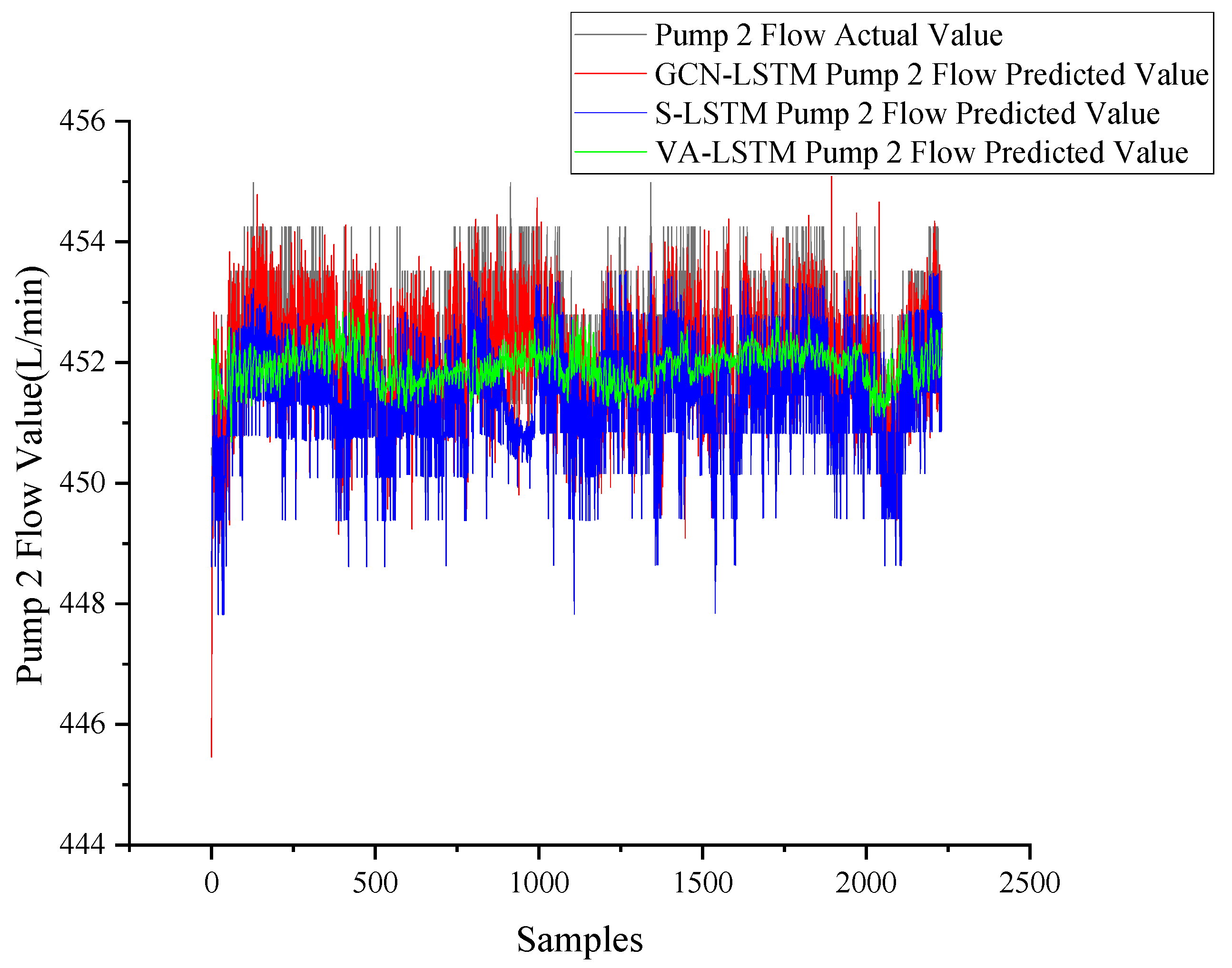
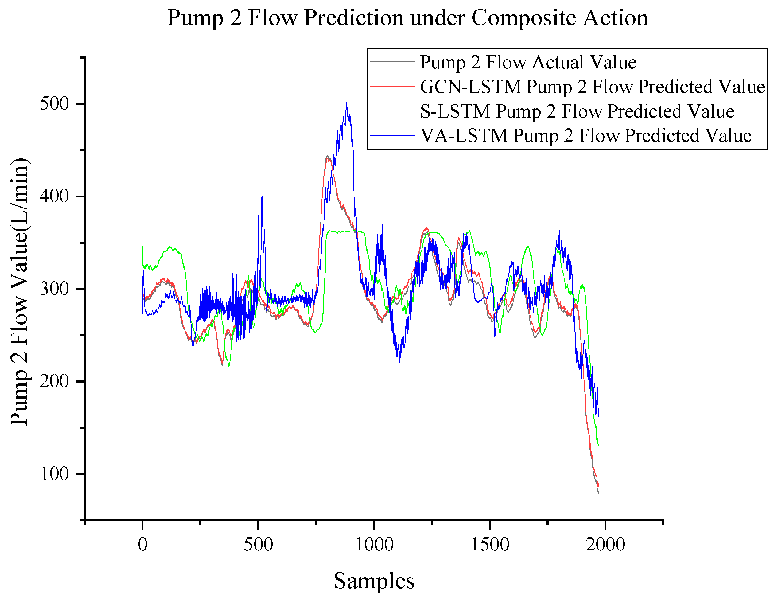
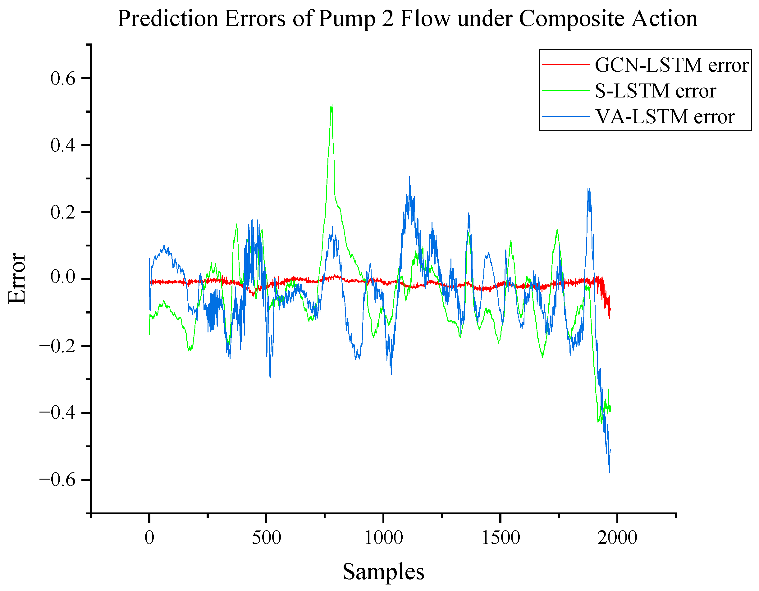
Figure 17 and Figure 18 depict the prediction and errors of pump 2 flow using the GCN-LSTM, S-LSTM, and VA-LSTM models on the testing dataset, respectively. Once again, the prediction curves generated by the GCN-LSTM model exhibit a close alignment with the real output curves. In contrast, there are significant deviations between the real and predicted output curves for the S-LSTM and VA-LSTM models. The predicted errors for the S-LSTM and VA-LSTM networks mostly fall within the range of [−0.6, 0.6]. However, the GCN-LSTM model shows substantially smaller prediction errors, mostly centered around zero. This indicates that the GCN-LSTM model performs better in terms of accuracy when predicting pump 2 flow compared to the S-LSTM and VA-LSTM models.

3.5. Public Datasets

To validate the effectiveness and performance of our proposed GCN-LSTM soft sensor model in non-hydraulic pump applications, we applied the method to the sulfur recovery dataset [53] and the debutanizer column dataset [54], both of which are public datasets used for soft sensor modeling.

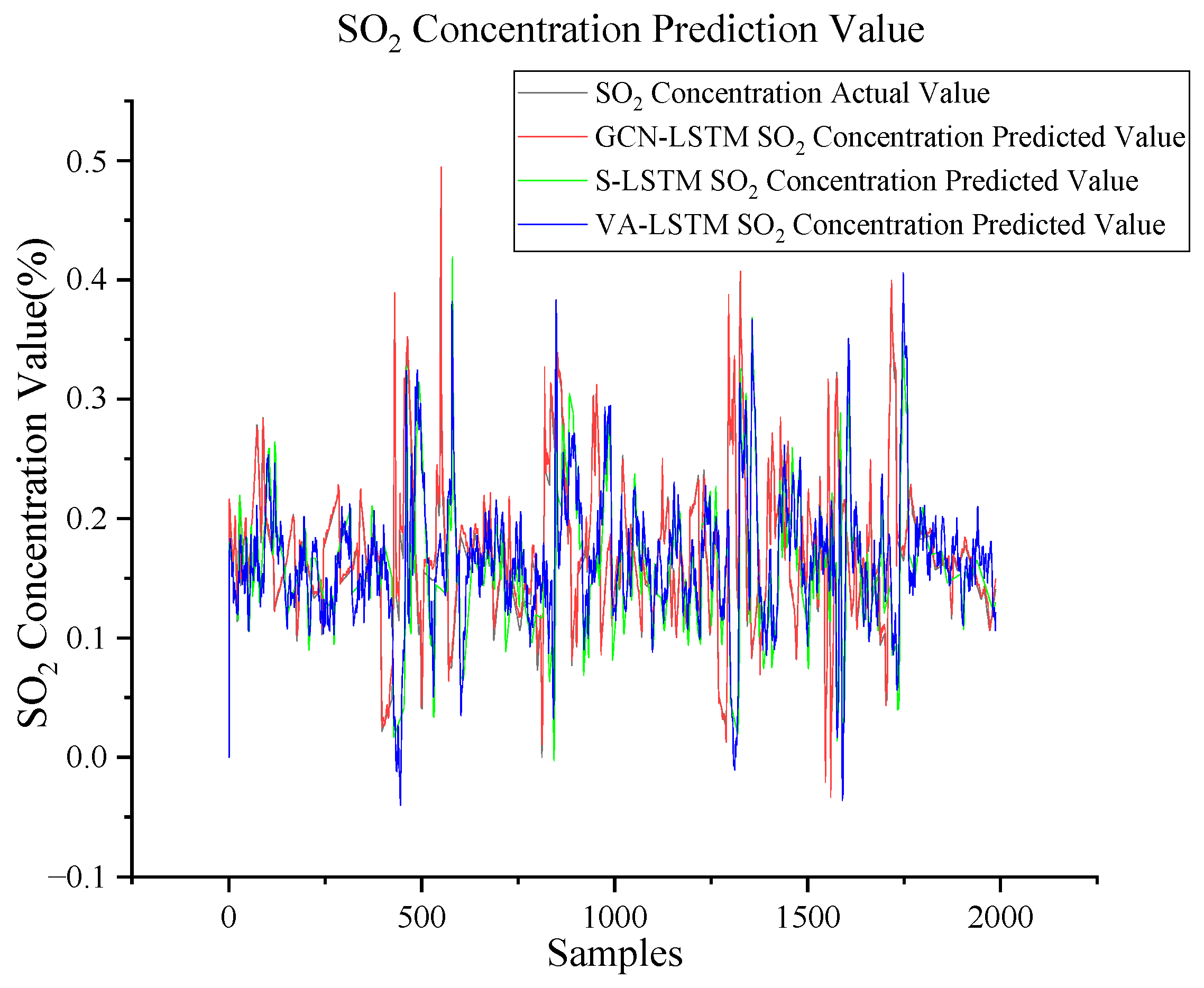
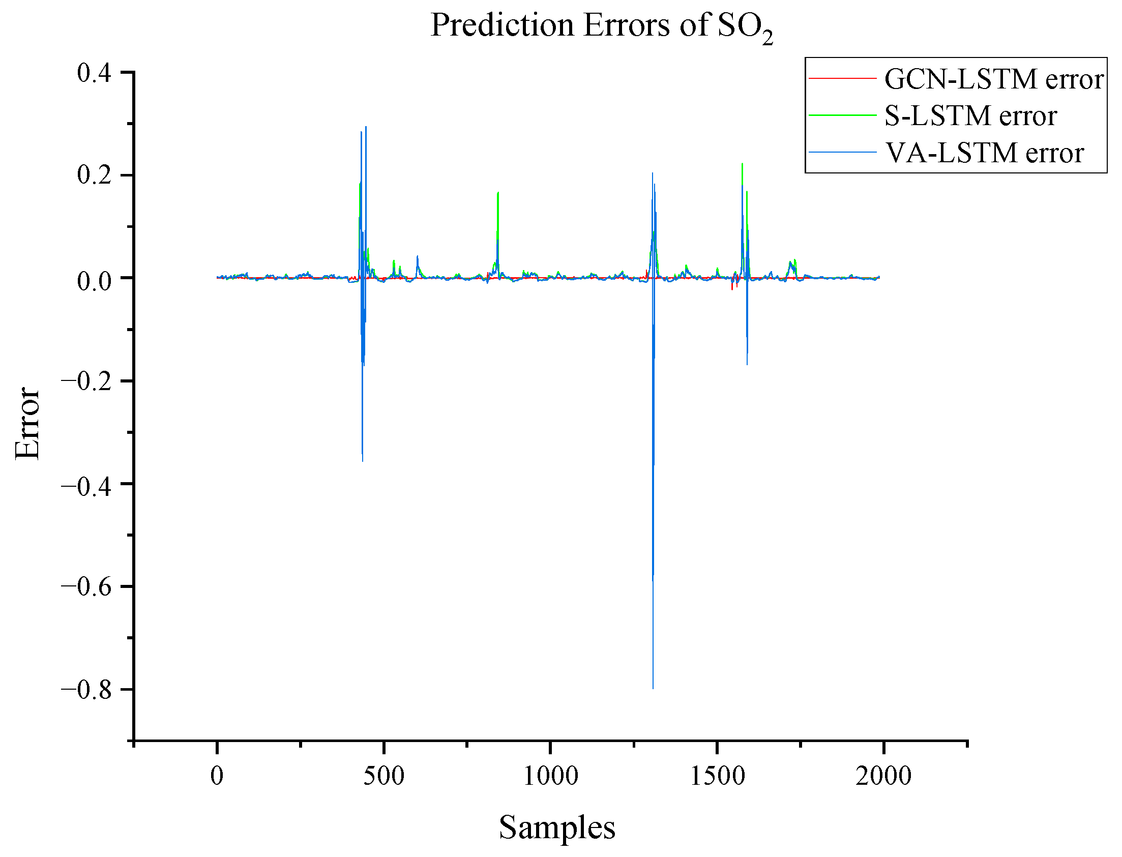
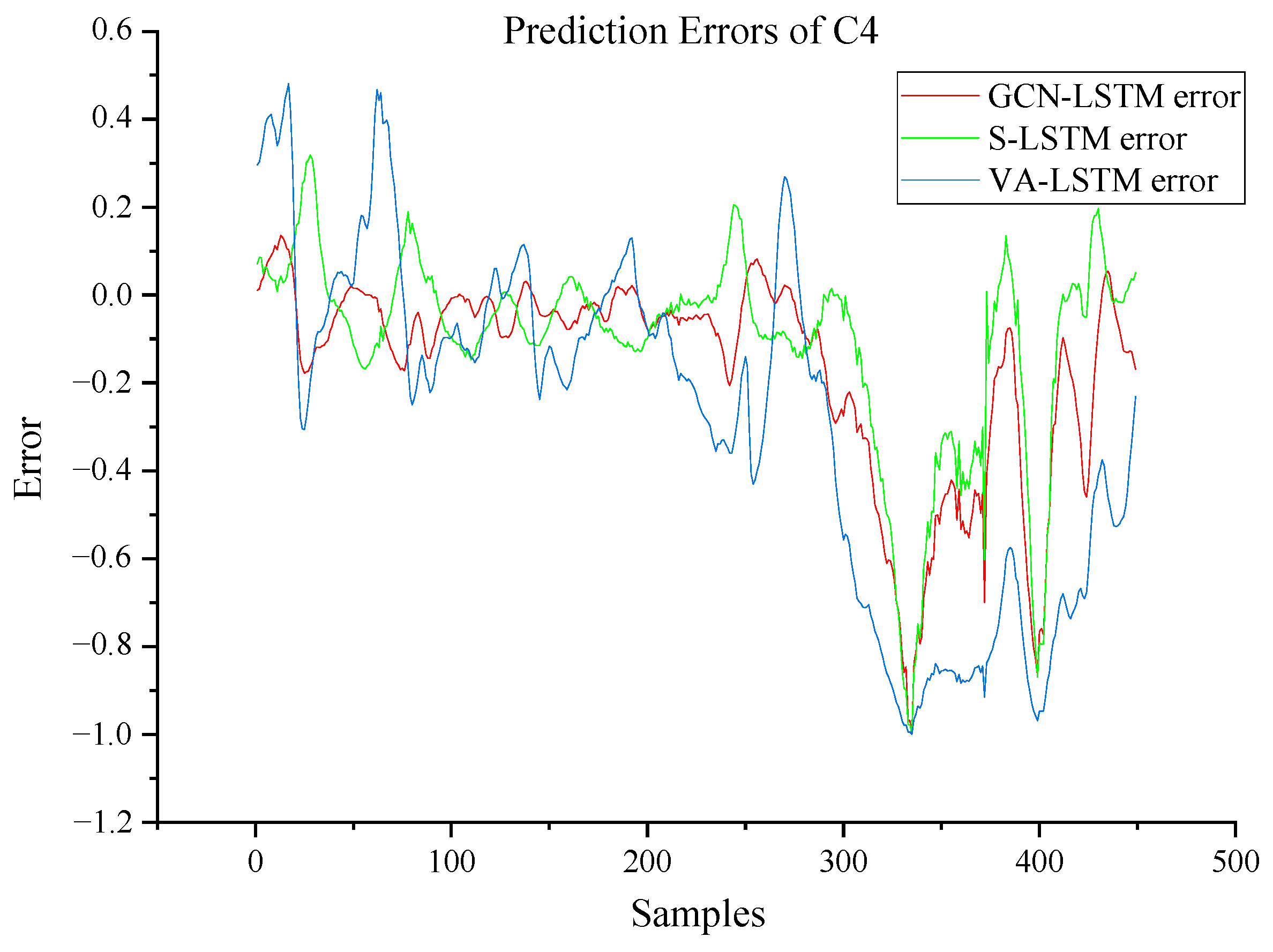
Figure 19 and Figure 20 depict the prediction and errors of SO2 in the sulfur recovery dataset using the GCN-LSTM, S-LSTM, and VA-LSTM models on the testing dataset, respectively. The GCN-LSTM model demonstrates excellent tracking with the real output curves and exhibits significantly smaller prediction errors compared to the other models. Similarly, Figure 21 and Figure 22 depict similar results for the prediction and errors of C4 in the debutanizer column dataset, further highlighting the superior performance of the GCN-LSTM model.

4. Discussion and Results

In the case of the steady-state condition for the swing and walking actions of the hydraulic shovel, there is no significant difference in the predictive performance of the GCN-LSTM, S-LSTM, and VA-LSTM models for the flow prediction of pump 1 and pump 2. However, for the excavation composite action under variable operating conditions, the GCN-LSTM model clearly outperforms the S-LSTM and VA-LSTM models in terms of flow prediction for pump 1 and pump 2. This highlights the superior predictive performance of the GCN-LSTM model under complex operating conditions. To further evaluate the GCN-LSTM model, we conducted a comparative analysis using two indicators: the RMSE and R². The RMSE and R² values for the three soft sensors based on the swing action, walking action, and composite action conditions are presented in

Table 3. RMSE and R² of pump 1 flow, pump 2 flow, SO₂, and C4 based on S-LSTM, VA-LSTM, and GCN-LSTM.

Target Variables	Indicators	S-LSTM	VA-LSTM	GCN-LSTM
Swing action pump 2 flow	RMSE R2	0.1027 0.726	0.1262 0.703	0.0916 0.857
Walking action pump 1 flow	RMSE R2	0.1047 0.364	0.0921 0.754	0.0782 0.898
Composite action pump 1 flow	RMSE R2	0.0745 0.579	0.0903 0.386	0.0109 0.987
Composite action pump 2 flow	RMSE R2	0.0532 0.767	0.0742 0.547	0.0109 0.990
SO2	RMSE R2	0.0188 0.894	0.0236 0.833	0.0114 0.962
C4	RMSE R2	0.0404 0.962	0.1617 0.393	0.0357 0.971

.

In the case of pump 2 flow prediction based on the swing action, the GCN-LSTM model achieves an RMSE value of 0.0916 and an R² value of 0.857. Meanwhile, for pump 1 flow prediction based on the walking action, the RMSE value is 0.0782 and the R² value is 0.898. These RMSE and R² values indicate that the GCN-LSTM model performs significantly better than the S-LSTM and VA-LSTM models under the two steady-state operating conditions.

In the case of the composite action of hydraulic shovel excavation, which involves variable conditions, the flow of pump 1 and pump 2 dynamically changes with the executed action. For pump 1 flow prediction based on the composite action, the GCN-LSTM model achieves an RMSE value of 0.0109 and an R² value of 0.987. Similarly, for pump 2 flow prediction based on the composite action, the RMSE value is 0.0109 and the R² value is 0.990. These results demonstrate that the GCN-LSTM model continues to outperform the S-LSTM and VA-LSTM models, even under variable working conditions.

In the case of the sulfur recovery dataset, the GCN-LSTM model achieves an RMSE value of 0.0114 and an R² value of 0.962 for the prediction of SO₂. In the debutanizer column dataset, the RMSE value of the GCN-LSTM model is 0.0357 and the R² value is 0.971 for the prediction of C4. These results highlight the superior prediction performance of the GCN-LSTM model compared to the S-LSTM and VA-LSTM models in both non-hydraulic pump use cases. Overall, the GCN-LSTM model demonstrates significantly higher prediction accuracy than the S-LSTM and VA-LSTM models for both the sulfur recovery and debutanizer column datasets.

5. Conclusions

In this paper, a GCN-LSTM network is proposed for nonlinear dynamic modeling for soft sensor applications. The GCN is used to extract the spatial feature information of the process variables, and LSTM is used to extract the temporal feature information of the process variables. This enables the construction of deep networks for hierarchical nonlinear dynamic hidden feature descriptions, which are beneficial for the prediction of the target variables. The main conclusions are as follows:

(1)

The GCN-LSTM model outperformed the S-LSTM and VA-LSTM models in predicting the flow of hydraulic pumps under steady-state conditions (swing and walking actions) and variable operating conditions (composite action);

(2)

The GCN-LSTM model demonstrated superior predictive performance in the sulfur recovery and debutanizer column datasets compared to the S-LSTM and VA-LSTM models.

Overall, the GCN-LSTM model demonstrated superior predictive accuracy compared to the S-LSTM and VA-LSTM models across different scenarios, highlighting its potential for soft sensor applications in machinery systems.

Regarding future research:

(1)

The GCN-LSTM model is highly sensitive to the quality and quantity of data. Therefore, the introduction of more advanced data preprocessing techniques to reduce noise interference in the data is an area that requires further research;

(2)

Given the high computational complexity of the GCN-LSTM model, optimizing its structure to reduce the number of parameters is an important direction for future research.

References

1. Wang, S.H.; Xiang, J.W.; Zhong, Y.T. A data indicator-based deep belief networks to detect multiple faults in axial piston pumps. Mech. Syst. Signal Process. 2018, 112, 154–170. [Google Scholar] [CrossRef]
2. He, Y.; Tang, H.S.; Kumar, A. A deep multi-signal fusion adversarial model-based transfer learning and residual network for axial piston pump fault diagnosis. Measurement 2022, 192, 110889. [Google Scholar] [CrossRef]
3. Zhu, Y.; Li, G.P.; Wang, R. Intelligent fault diagnosis of hydraulic piston pump combining improved LeNet-5 and PSO hyperparameter optimization. Appl. Acoust. 2021, 183, 108336. [Google Scholar] [CrossRef]
4. Yu, H.; Li, H.R.; Li, Y.L. Vibration signal fusion using improved empirical wavelet transform and variance contribution rate for weak fault detection of hydraulic pumps. ISA Trans. 2020, 107, 385–401. [Google Scholar] [CrossRef] [PubMed]
5. Chen, X.R.; Liu, H.; Nikitas, N. Internal pump leakage detection of the hydraulic systems with highly incomplete flow data. Adv. Eng. Inform. 2023, 56, 101974. [Google Scholar] [CrossRef]
6. Wu, Y.Z.; Wu, D.H.; Fei, M.H. Application of GA-BPNN on estimating the flow rate of a centrifugal pump. Eng. Appl. Artif. Intel. 2023, 119, 105738. [Google Scholar] [CrossRef]
7. Yao, L.; Shen, B.B.; Cui, L.L. Semi-Supervised Deep Dynamic Probabilistic Latent Variable Model for Multimode Process Soft Sensor Application. IEEE Trans. Ind. Inform. 2023, 19, 6056–6068. [Google Scholar] [CrossRef]
8. Gao, S.W.; Qiu, S.L.; Ma, Z.Y. SVAE-WGAN-Based Soft Sensor Data Supplement Method for Process Industry. IEEE Sens. J. 2022, 22, 601–610. [Google Scholar] [CrossRef]
9. Nie, L.; Ren, Y.Z.; Wu, R.H. Sensor Fault Diagnosis, Isolation, and Accommodation for Heating, Ventilating, and Air Conditioning Systems Based on Soft Sensor. Actuators. 2023, 12, 389. [Google Scholar] [CrossRef]
10. Gao, S.W.; Zhang, Q.S.; Tian, R. Collaborative Apportionment Noise-Based Soft Sensor Framework. IEEE Trans. Instrum. Meas. 2022, 71, 1–12. [Google Scholar] [CrossRef]
11. Yuan, X.F.; Li, L.; Wang, Y.L. Deep Learning with Spatiotemporal Attention-Based LSTM for Industrial Soft Sensor Model Development. IEEE Trans. Ind. Electron. 2021, 68, 4404–4414. [Google Scholar] [CrossRef]
12. Guo, R.Y.; Liu, H.; Xie, G. A Self-Interpretable Soft Sensor Based on Deep Learning and Multiple Attention Mechanism: From Data Selection to Sensor Modeling. IEEE Trans. Ind. Inform. 2023, 19, 6859–6871. [Google Scholar] [CrossRef]
13. Xie, W.; Wang, J.S.; Xing, C. Variational Autoencoder Bidirectional Long and Short-Term Memory Neural Network Soft-Sensor Model Based on Batch Training Strategy. IEEE Trans. Ind. Inform. 2023, 17, 5325–5334. [Google Scholar] [CrossRef]
14. Mannering, F.; Bhat, C.R.; Shankar, V. Big data, traditional data and the tradeoffs between prediction and causality in highway-safety analysis. Anal. Methods Accid. Res. 2020, 25, 100113. [Google Scholar] [CrossRef]
15. Shen, B.W.; Yao, L.; Ge, Z. Nonlinear probabilistic latent variable regression models for soft sensor application: From shallow to deep structure. Control Eng. Pract. 2020, 94, 100113. [Google Scholar] [CrossRef]
16. Ferreira, J.; Pedemonte, M.; Torres, A.I. Development of a machine learning-based soft sensor for an oil refinery’s distillation column. Comput. Chem. Eng. 2022, 161, 107756. [Google Scholar] [CrossRef]
17. Xibilia, M.G.; Latino, M.; Marinkovic, Z. Soft sensors based on deep neural networks for applications in security and safety. IEEE Trans. Instrum. Meas. 2020, 69, 7869–7876. [Google Scholar] [CrossRef]
18. Zheng, J.H.; Song, Z.H. Semisupervised learning for probabilistic partial least squares regression model and soft sensor application. J. Process Control 2018, 64, 123–131. [Google Scholar] [CrossRef]
19. Herceg, S.; Andriji’c, Ž.U.; Bolf, N. Development of soft sensors for isomerization process based on support vector machine regression and dynamic polynomial models. Chem. Eng. Res. Design 2019, 149, 95–103. [Google Scholar] [CrossRef]
20. Wang, G.M.; Jia, Q.S.; Zhou, M.C. Artificial neural networks for water quality soft-sensing in wastewater treatment: A review. Artif. Intell. Rev. 2021, 55, 565–587. [Google Scholar] [CrossRef]
21. Zhu, P.B.; Liu, X.Y.; Wang, B. Mixture semisupervised Bayesian principal component regression for soft sensor modeling. IEEE Access. 2018, 6, 40909–40919. [Google Scholar] [CrossRef]
22. Li, W.Q.; Yang, C.H.; Jabari, S.E. Nonlinear traffic prediction as a matrix completion problem with ensemble learning. Transp. Sci. 2022, 56, 52–78. [Google Scholar] [CrossRef]
23. Lima, J.M.M.; Araujo, F.M.U. Ensemble deep relevant learning framework for semi-supervised soft sensor modeling of industrial processes. Neurocomputing 2021, 462, 154–168. [Google Scholar] [CrossRef]
24. Chai, Z.; Zhao, C.H.; Huang, B. A Deep Probabilistic Transfer Learning Framework for Soft Sensor Modeling with Missing Data. IEEE Trans. Neural Netw. Learn. Syst. 2022, 33, 7598–7609. [Google Scholar] [CrossRef] [PubMed]
25. Sun, Q.Q.; Ge, Z.Q. A survey on deep learning for data-driven soft sensors. IEEE Trans. Ind. Informat. 2021, 17, 5853–5866. [Google Scholar] [CrossRef]
26. Zheng, J.H.; Wu, C.; Sun, Q.Q. Deep learning of complex process data for fault classification based on sparse probabilistic dynamic network. J. Taiwan Inst. Chem. Eng. 2022, 138, 104498. [Google Scholar] [CrossRef]
27. Yuan, X.F.; Qi, S.B.; Wang, Y.L. A dynamic CNN for nonlinear dynamic feature learning in soft sensor modeling of industrial process data. Control Eng. Pract. 2020, 104, 104614. [Google Scholar] [CrossRef]
28. Gilbert Chandra, D.; Vinoth, B.; Srinivasulu Reddyb, U. Recurrent Neural Network based Soft Sensor for flow estimation in Liquid Rocket Engine Injector calibration. Flow Meas. Instrum. 2022, 83, 102105. [Google Scholar]
29. Ke, W.S.; Huang, D.X.; Yang, F. Soft sensor development and applications based on LSTM in deep neural networks. Proc. IEEE Symp. Ser. Comput. Intell. 2017, 12, 1–6. [Google Scholar]
30. Sun, Q.Q.; Ge, Z.Q. Gated Stacked Target-Related Autoencoder: A Novel Deep Feature Extraction and Layerwise Ensemble Method for Industrial Soft Sensor Application. IEEE Trans. Cybern. 2022, 52, 3457–3468. [Google Scholar] [CrossRef]
31. Fan, W.; Si, F.Q.; Ren, S.J. Integration of continuous restricted Boltzmann machine and SVR in NOx emissions prediction of a tangential firing boiler. Chemom. Intell. Lab. Syst. 2019, 195, 103870. [Google Scholar] [CrossRef]
32. Yuan, X.F.; Qi, S.B.; Wang, Y.L. Soft sensor model for dynamic processes based on multichannel convolutional neural network. Chemom. Intell. Lab. Syst. 2020, 203, 104050. [Google Scholar] [CrossRef]
33. Alghamdi, W.Y. A novel deep learning method for predicting athletes’ health using wearable sensors and recurrent neural networks. Decis. Anal. J. 2023, 7, 100213. [Google Scholar] [CrossRef]
34. Jorge, L.B.; Heo, S.K.; Yoo, C.K. Soft sensor validation for monitoring and resilient control of sequential subway indoor air quality through memory-gated recurrent neural networks-based autoencoders. Control Eng. Pract. 2020, 97, 104330. [Google Scholar]
35. Zhu, K.; Zhao, C.H. Dynamic Graph-Based Adaptive Learning for Online Industrial Soft Sensor with Mutable Spatial Coupling Relations. IEEE Trans. Ind. Electron. 2023, 70, 9614–9622. [Google Scholar] [CrossRef]
36. Song, P.Y.; Zhao, C.H. Slow down to go better: A survey on slow feature analysis. IEEE Trans. Neural Netw. Learn. Syst. 2022, 326, 1–21. [Google Scholar] [CrossRef] [PubMed]
37. Chen, Y.; Chen, X.Q. A novel reinforced dynamic graph convolutional network model with data imputation for network-wide traffic flow prediction. Transp. Res. C Emerg. Technol. 2022, 143, 103820. [Google Scholar] [CrossRef]
38. Wang, G.T.; Zhang, Z.R.; Bian, Z.P. A short-term voltage stability online prediction method based on graph convolutional networks and long short-term memory networks. Int. J. Elec. Power. 2021, 127, 103820. [Google Scholar] [CrossRef]
39. Ta, X.X.; Liu, Z.H.; Hu, X. Adaptive Spatio-temporal Graph Neural Network for traffic forecasting. Knowl.-Based Syst. 2022, 242, 108199. [Google Scholar] [CrossRef]
40. Yu, B.; Yin, H.T.; Zhu, Z.X. Spatio-temporal graph convolutional networks: A deep learning framework for traffic forecasting. In Proceedings of the IJCAI-27, 27th International Joint Conference on Artificial Intelligence, Stockholm, Sweden, 13–19 July 2018; pp. 3634–3640. [Google Scholar]
41. Wang, X.; Zhu, M.Q.; Bo, D.Y. AM-GCN: Adaptive Multi-channel Graph Convolutional Networks. In Proceedings of the KDD-20, 26th ACM SIGKDD International Conference on Knowledge Discovery & Data Mining, Virtual, 6–10 July 2020; pp. 1243–1253. [Google Scholar]
42. Zhou, K.B.; Yang, C.Y.; Liu, J. Dynamic graph-based feature learning with few edges considering noisy samples for rotating machinery fault diagnosis. IEEE Trans. Ind. Electron. 2022, 69, 10595–10604. [Google Scholar] [CrossRef]
43. Yang, C.Y.; Liu, J.; Zhou, K.B. An improved multi-channel graph convolutional network and its applications for rotating machinery diagnosis. Measurement 2022, 190, 110720. [Google Scholar] [CrossRef]
44. Jiang, Y.C.; Yin, S.; Dong, J.W. A Review on Soft Sensors for Monitoring, Control, and Optimization of Industrial Processes. IEEE Sens. J. 2021, 21, 12868–12881. [Google Scholar] [CrossRef]
45. Li, X.T.; Michael, K.N.; Xu, G.N. Multi-channel fusion graph neural network for multivariate time series forecasting. Neural Netw. 2023, 161, 343–358. [Google Scholar] [CrossRef] [PubMed]
46. Hu, Z.N.; Dong, Y.X.; Wang, K.S. GPT-GNN: Generative Pre-Training of Graph Neural Networks. In Proceedings of the KDD-20, 26th ACM SIGKDD International Conference on Knowledge Discovery & Data Mining, Virtual Event, CA, USA, 6–10 July 2020; Volume 56, pp. 1857–1867. [Google Scholar]
47. Park, M.Y.; Geum, Y.J. Two-stage technology opportunity discovery for firm-level decision making: GCN-based link-prediction approach. Technol. Forecast. Soc. Chang. 2022, 183, 121934. [Google Scholar] [CrossRef]
48. Lui, C.F.; Liu, Y.; Xie, M. A Supervised Bidirectional Long Short-Term Memory Network for Data-Driven Dynamic Soft Sensor Modeling. IEEE Trans. Instrum. Meas. 2022, 71, 1–13. [Google Scholar] [CrossRef]
49. Huang, D.Y.; Liu, H.; Bi, T.S. GCN-LSTM spatiotemporal-network-based method for post-disturbance frequency prediction of power systems. Glob. Energy Interconnect. 2022, 5, 96–107. [Google Scholar] [CrossRef]
50. Yuan, X.F.; Huang, B.; Wang, Y.L. Deep Learning-Based Feature Representation and Its Application for Soft Sensor Modeling with Variable-Wise Weighted SAE. IEEE Trans. Ind. Inform. 2018, 14, 3235–3243. [Google Scholar] [CrossRef]
51. Yuan, X.F.; Li, L.; Wang, Y.L. Nonlinear dynamic soft sensor modeling with supervised long short-term memory network. IEEE Trans. Ind. Inform. 2019, 16, 3168–3176. [Google Scholar] [CrossRef]
52. Yuan, X.F.; Li, L.; Wang, Y.L. Deep learning for quality prediction of nonlinear dynamic processes with variable attention- based long short-term memory network. Can. J. Chem. Eng. 2020, 98, 1377–1389. [Google Scholar] [CrossRef]
53. Fortuna, L.; Rizzo, A.; Sinatra, M. Soft analyzers for a sulfur recovery unit. Control Eng. Pract. 2003, 11, 1491–1500. [Google Scholar] [CrossRef]
54. Yuan, X.F.; Ou, C.; Wang, Y.L. A novel semi-supervised pre-training strategy for deep networks and its application for quality variable prediction in industrial processes. Chem. Eng. Sci. 2020, 2017, 115509. [Google Scholar] [CrossRef]
Figure 1. The network diagram of the GCN with input layer, hidden layers, and output layer. (The green nodes generate blue nodes after being processed by the ReLU function).
Actuators 13 00038 g001
Figure 2. LSTM network architecture diagram.
Actuators 13 00038 g002
Figure 3. GCN-LSTM prediction process diagram.
Actuators 13 00038 g003
Figure 4. GCN-LSTM training and testing process diagram.
Actuators 13 00038 g004
Figure 5. Simplified diagram of the walking hydraulic system (1. Pump 1; 2, 6, 7, 8, 9, 16, 18. Overflow valve; 3, 15. Check valve; 4, 13. Main valve; 5, 10. Walk motor; 11, 12. Joystick; 14. Pilot valve; 17. Pump 2; 19. Pilot pump; 20. Oil tank).
Actuators 13 00038 g005
Figure 6. Simplified diagram of the swing hydraulic system (1. Pump 2; 2, 5, 6, 8, 9, 13. Overflow valve; 3. Check valve; 4. Main valve; 7, 10. Swing motor; 11. Joystick; 12. Pilot valve; 14. Pilot pump; 15. Oil tank).
Actuators 13 00038 g006
Figure 7. Simplified diagram of the boom hydraulic system (1. Pump 1; 2. Pump 2; 3, 4. Check valve; 5. Main valve; 6, 9. Boom cylinder; 7, 8. Balance valve; 10. Joystick; 11. Pilot valve; 12, 14. Overflow valve; 13. Pilot pump; 15. Oil tank).
Actuators 13 00038 g007
Figure 8. Simplified diagram of the arm hydraulic system (1. Pump 1; 2. Pump 2; 3, 4. Check valve; 5. Main valve; 6. Balance valve; 7. Arm cylinder; 8. Joystick; 9. Pilot valve; 10, 12. Overflow valve; 11. Pilot pump; 13. Oil tank).
Actuators 13 00038 g008
Figure 9. Simplified diagram of the bucket hydraulic system (1. Pump 1; 2. Pump 2; 3, 4. Check valve; 5. Main valve; 6. Bucket cylinder; 7. Joystick; 8. Pilot valve; 9, 11. Overflow valve; 10. Pilot pump; 12. Oil tank).
Actuators 13 00038 g009
Figure 10. Installation diagram of variable acquisition sensors for hydraulic shovels.
Actuators 13 00038 g010
Figure 11. Pump 2 flow prediction under swing action based on GCN-LSTM, S-LSTM, and VA-LSTM.
Actuators 13 00038 g011
Figure 12. Prediction errors of pump 2 flow prediction under swing action based on GCN-LSTM, S-LSTM, and VA-LSTM.
Actuators 13 00038 g012
Figure 13. Pump 1 flow prediction under walking action based on GCN-LSTM, S-LSTM, and VA-LSTM.
Actuators 13 00038 g013
Figure 14. Prediction errors of pump 1 flow under walking action based on GCN-LSTM, S-LSTM, and VA-LSTM.
Actuators 13 00038 g014
Figure 15. Pump 1 flow prediction under composite action based on GCN-LSTM, S-LSTM, and VA-LSTM.
Actuators 13 00038 g015
Figure 16. Prediction errors of pump 1 flow under composite action based on GCN-LSTM, S-LSTM, and VA-LSTM.
Actuators 13 00038 g016
Figure 17. Pump 2 flow prediction under composite action based on GCN-LSTM, S-LSTM, and VA-LSTM.
Actuators 13 00038 g017
Figure 18. Prediction errors of pump 2 flow under composite action based on GCN-LSTM, S-LSTM, and VA-LSTM.
Actuators 13 00038 g018
Figure 19. SO2 concentration prediction value based on GCN-LSTM, S-LSTM, and VA-LSTM.
Actuators 13 00038 g019
Figure 20. Prediction errors of SO2 based on GCN-LSTM, S-LSTM, and VA-LSTM.
Actuators 13 00038 g020
Figure 21. C4 concentration prediction value based on GCN-LSTM, S-LSTM, and VA-LSTM.
Actuators 13 00038 g021
Figure 22. Prediction errors of C4 based on GCN-LSTM, S-LSTM, and VA-LSTM.
Actuators 13 00038 g022