Prediction and Control of Small Deviation in the Time-Delay of the Image Tracker in an Intelligent Electro-Optical Detection System

Abstract

A small deviation in the time-delay of the image tracker is essential for improving the tracking precision of an electro-optical system, and for future advances in actuator technology. The core goal of this manuscript is to address issues such as tracking the controller time-delay compensation and the precision of an electro-optical detection system using an advanced filter design, a fire control modeling, and an anti-occlusion target detection system. To address this problem, a small deviation in the time-delay prediction and control method of the image tracker is proposed based on the principle of linear motion transformation. The time-delay error formation is analyzed in detail to reveal the scientific mechanism between the tracking controller feedback and the line-of-sight position correction. An advanced N-step Kalman filtering controller model is established by combining a line-of-sight firing control judgment and a single-sample training anti-occlusion DSST target tracking strategy. Finally, an actuator platform with three degrees of freedom is used to test the optical mechatronics system. The results show that the distribution probability of the line-of-sight measuring error in a circle with a radius of 0.15 mrad is 72%. Compared with the traditional control method, the tracking precision of the optimal method is improved by 58.3%.

1. Introduction

Unmanned equipment, which denotes intelligent precision devices with the specific functions of reconnaissance, positioning, aiming, and target tracking [1,2,3,4,5], plays an increasingly important role in actuator technology and industry. With the capability of target imaging, labeling, tracking, and measuring, an electro-optical detection system (EODS) is an essential component in unmanned equipment for conducting autonomous target recognition, aiming, and tracking.

EODS is generally equipped with a tracking controller, which is used to calculate the miss-distance between the center of the target position and the center of the lens field-view in real time. It is also equipped with a judgment controller to select the firing time based on the miss-distance [6]. The core performance measure of an EODS is its targeting precision, especially for “low, slow and small (LSS)” fast-moving targets [7]. The specific performance indicators of the target are a distance of less than 500 m, area of less than 2 m², and speed of 30~50 m/s [8]. In this case, the targeting precision of the EODS should be less than 0.15 mrad to accurately hit the target. To satisfy such a requirement, the dynamic performance of the line-of-sight (LOS) of an EODS, i.e., the stability response time, must be ensured. However, due to the intrinsic properties of the digital imaging systems of an EODS, time delay is one of the main obstacles to improving the EODS dynamics thus affecting the tracking and aiming performance of the electro-optical equipment.

The miss-distance can only be measured after the establishment, processing, and transmission of image signals, so the target miss-distance obtained by the controller will lag behind the actual target imaging time. Therefore, there is a small deviation between the measured value and the true value caused by the tracker time-delay, which can lead to a decrease in tracking precision. According to the definition of the Society of Photo-Optical Instrumentation Engineers (SPIE), small is considered to be an area of less than 80 pixels in a 256 × 256 image. This indicates that less than 0.12% of the image resolution is a small target [9]. And the EODS needs to control this deviation within 1~3 pixels in a lens of 1280 × 720 pixels for long-distance precision shooting. Thus, the deviation to be corrected in target tracking and aiming is very tiny.

However, as a small deviation detection element, the precision of the existing image trackers is not high enough. The time-delay error of a tracker is also affected by the frame rate, lens resolution, and hardware circuit. Thus, it will delay the best firing time and even result in lower tracking precision.

There are two kinds of traditional ways to improve precision. The first type involves improving the performance of the tracking algorithm. Tomar et al. [10] proposed a dynamic kernel convolution neural network linear regression model to track people under dense occlusion. Lin et al. [11] proposed an intelligent hybrid strategy based on machine vision for detecting a mechanical work piece. The test showed that the tracking error was less than 0.06 mm. However, most deep learning methods require high image quality, and it takes a lot of sample data and training time to obtain a barely suitable detection model. In actual gun firing, the tracking data should be obtained quickly, and the image detection will be affected by an adverse environment, such as light intensity, lens dust, scratches, and target occlusion. Thus, these methods are not suitable for EODS tracking and aiming. Wu et al. [12] proposed a gray-level feature dual-neighbor gradient method. Han et al. [13] proposed a multi-scale three-layer local gray-level contrast metric tracking detection framework. The advantage of these template matching methods is that they can complete the tracking without a lot of sample data. But it is easy to lose the target position after its occlusion or a change in direction.

The second type involves keeping the tracking algorithm unchanged and introducing an advanced filter prediction technology. The US Air Force has designed a three-state filter for the “AH-64 Apache” helicopter to obtain the predicted speed value. A good filter prediction method can break through the limit of the image algorithm and improve the tracking precision. Wen et al. [14] proposed a direct integration method for time-delay control. Malviya et al. [15] proposed a particle filter with a robotic arm. Zhong et al. [16] established a passive error feature prediction equation based on the geometric dynamics of a spherical camera. Wu et al. [17] proposed a nonlinear Gaussian iterative prediction model to achieve the visual servo stability control of wheeled robots. Zhang et al. [18] fused the inertial measurement unit and monocular camera, and adopted the iterative extended Kalman filter. The tests showed that the accuracy was improved by 15–30 times. However, these filter prediction methods are mainly used for servo mechanisms or long-range rotation, and the overall structure weight is too large. Moreover, the manual aiming and tracking action belong to low-frequency, small-amplitude, and short-range motion within 1.5 Hz. Thus, these methods are not convenient for operators to quickly deploy and carry out.

According to the above representative sample of recent studies on image processing and filter prediction, there are still only a few types of small deviation time-delay prediction methods for image trackers in EODS firing, and a control method with high tracking precision is still in the exploratory stage.

The core goal of this paper is to address issues such as tracking controller time-delay compensation and tracking precision of an electro-optical detection system using an advanced filter design, fire control modeling, and anti-occlusion target detection. In response to this problem, a small deviation time-delay prediction and control method for an image tracker is proposed based on the aim of linear motion transformation. The time-delay error formation is analyzed in detail to reveal the scientific mechanism between the tracking controller feedback and the line-of-sight position correction. An advanced N-step Kalman filtering controller model is established by combining a line-of-sight firing control judgment and a single-sample training anti-occlusion DSST target tracking strategy. The experiment shows that the distribution probability of the line-of-sight measured error in a circle with a radius of 0.15 mrad is 72%. Compared with the traditional control method, the tracking precision of the optimal method are improved by 58.3%.

This manuscript is valuable for all the researchers who are interested in the electro-optical system, small deviation control, image tracker, and time-delay prediction.

2. Materials and Methods

2.1. Composition and Framework of EODS

The optical-mechatronics composition of an EODS is shown in Figure 1. As seen in the figure, the composition of the EODS includes a white light lens, an infrared lens, a laser range finder lens, an eyepiece and a collimated beam. The EODS is installed on a precision rotating platform. A Cassegrain collimator with the reticle is provided to simulate the infinity target and it also provides a reticle imaging observation point for the EODS.

The framework of the optical-mechatronics system of an EODS, along with a Cassegrain collimator, a light source detector and a target manipulator is shown in Figure 2. The light source detector is used to detect the laser offset distance on the target board.

2.2. Traditional Tracking Controller Model of an EODS

Figure 3 shows the traditional tracking controller model of an EODS. The tracker obtains the target resolution coordinate after collecting the image. Then, it calculates the miss-distance Δ between the target coordinate and the center coordinate of field view. The miss-distance is the angle deviation obtained by converting the number of pixels K, the lens resolution E × F, and the lens field angle $\alpha \times \beta$. The unit of miss-distance Δ is mrad. The qualitative relationship of error correction can be thus obtained.

(1)

Under the ideal condition without time-delay error of the tracker, the LOS position is the miss-distance Δ.

(2)

Under the actual condition with time-delay error of the tracker, the miss-distance Δ after tracker processing is the measured value of the LOS. There is a small deviation δ between the measured value and the true value of the LOS.

(3)

The core goal of this manuscript is to reduce the adverse impact of small deviation δ on the EODS and improve the tracking precision.

2.3. Optimized Model of the Tracking Controller in an EODS with Small Deviation in Time-Delay

As shown in Figure 4, the optimized tracking controller model of an EODS is established in this paper.

(1)

Model composition: Lens assembly, image tracker, prediction filter and firing controller. The model inputs the target image and outputs the LOS’s position.

(2)

Lens assembly: It collects the target image and generates a video stream with a frame rate of 25 Hz and a resolution of 1280 × 720 pixels (M × N). Then, it inputs the image tracker to extract a target’s features.

(3)

Image tracker: The DSST tracker inputs video stream and outputs a gray level feature response value $Z_{\max }$. The resolution coordinate ${\Delta }_{\mathrm{Z}}(x,y)$ corresponding to the response value $Z_{\max }$ is the target-tracking area of the current frame.

(4)

Prediction filter: An advanced N-step Kalman prediction filter is used to correct the small deviation in the time-delays ${\tau }_{\mathrm{T}}$ and ${\tau }_{\mathrm{G}}$. T is the sampling period. N is the fixed step. The estimated value of the next NT moment can be predicted after the correction. The LOS’s predicted value ${\widehat{X}}_f\left(t\right)$ is obtained via continuous recursive iteration.

(5)

Firing controller: It judges whether the LOS’s predicted value ${\widehat{X}}_f\left(t\right)$ coincide with the target’s actual position X(t). The small deviation δ will be limited within $\Delta -{\Delta }_0$.

Assume that the LOS’s true value is X(t). If the image tracker has a time-delay ${\tau }_{\mathrm{T}}$ and noise N, the quantitative relationship of the LOS’s measured value $X_{\mathrm{T}}(t)$ can be obtained.

$$X_{\mathrm{T}}(t)=X(t-{\tau }_{\mathrm{T}})+N$$

(1)

The time-delay of the tracker is generally about 1~3 frames. Suppose the noise N follows a normal distribution of zero mean. There are two main aspects of noise. One is the sensor-inherent noise and the other is ambient noise in the tracking target.

Assume that the firing threshold value is ${\Delta }_0$. When the measured value meets $X_{\mathrm{T}}(t)>{\Delta }_0$, it is judged that the LOS does not coincide with the target at this time. When $X_{\mathrm{T}}(t)\le {\Delta }_0$, it is judged that the LOS coincides with the target. The coincidence time is recorded as $t_{\mathrm{s}}$. So the currently measured value is marked as $X_{\mathrm{T}}(t_{\mathrm{s}})$. There is a time-delay ${\tau }_{\mathrm{G}}$ between the tracker receiving the coinciding signal and completing the firing. The firing time is recorded as $t_{\mathrm{e}}$. In Equation (2), the currently measured value is marked as $X_{\mathrm{T}}(t_{\mathrm{e}})$.

$$X_{\mathrm{T}}(t_{\mathrm{e}})=X_{\mathrm{T}}(t_{\mathrm{s}}+{\tau }_{\mathrm{G}})$$

(2)

The measured value $X_{\mathrm{T}}(t_{\mathrm{s}})$ is set as the standard when the miss-distance Δ reaches the given firing threshold value ${\mathsf{\Delta }}_0$. Then, time $t_{\mathrm{s}}$ is set as the standard. By comparing with the true value $X_{\mathrm{T}}(t_{\mathrm{s}})$, the quantitative relationship of small deviation δ can be obtained.

$$\begin{array}{ll}\delta & =X(t_{\mathrm{e}})-X_{\mathrm{T}}(t_{\mathrm{s}})\\ & =X(t_{\mathrm{e}})-X_{\mathrm{T}}(t_{\mathrm{e}})+X_{\mathrm{T}}(t_{\mathrm{e}})-X_{\mathrm{T}}(t_{\mathrm{s}})\\ & ={\delta }_1+{\delta }_2\end{array}$$

(3)

Then, the quantitative relationship of small deviations ${\delta }_1$ and ${\delta }_2$ can be obtained.

$$\left\{\begin{array}{l}{\delta }_1=X(t_{\mathrm{e}})-X_{\mathrm{T}}(t_{\mathrm{e}})\\ {\delta }_2=X_{\mathrm{T}}(t_{\mathrm{e}})-X_{\mathrm{T}}(t_{\mathrm{s}})\end{array}\right.$$

(4)

Therefore, the small deviation in time-delay τ consists of two parts:

(1)

Time-delay ${\tau }_{\mathrm{T}}$: It tracks the target according to the miss-distance Δ at a certain time in the past. When studying the small deviation ${\delta }_1$ of the image tracker at time $t_{\mathrm{e}}$, the time-delay ${\tau }_{\mathrm{T}}$ should be subtracted. In Equation (1), the small deviation ${\delta }_1$ that is generated at time $t_{\mathrm{s}}-{\tau }_{\mathrm{T}}$ is corrected to reduce the adverse impact of time-delay on EODS firing.

(2)

Time-delay ${\tau }_{\mathrm{G}}$: It tracks the target according to the miss-distance Δ at a certain time in the future. The image tracker has a signal time-delay between coinciding time $t_{\mathrm{s}}$ and shooting time $t_{\mathrm{e}}$. The LOS is still shaky within the time-delay ${\tau }_{\mathrm{G}}$. When studying the small deviation ${\delta }_2$ of the image tracker at time $t_{\mathrm{e}}$, the time-delay ${\tau }_{\mathrm{G}}$ should be added. In Equation (2), the small deviation ${\delta }_2$ generated at time $t_{\mathrm{s}}+{\tau }_{\mathrm{G}}$ is corrected to reduce the adverse impact of time-delay on EODS firing.

3. Control Design

3.1. Miss-Distance Advanced Kalman Prediction Filtering Controller

In order to obtain the change in the LOS’s characteristics during target tracking and aiming of an EODS, the aiming linear motion transformation model is established. In actual shooting, the aiming and tracking action belong to a low frequency, small amplitude and a small range motion within 1.5 Hz. And the LOS’s motion of pitch and azimuth direction is basically the same, so the LOS’s jitter motion can be supposed into a linear motion transformation model.

The signal collection of a tracking controller is a discrete process. According to the general model of the random linear discrete system, the mathematical equations for an LOS’s motion state and the image tracker’s measured value can be obtained.

$$\left\{\begin{array}{l}{X}_k={\Phi }_{k|k-1}{X}_{k-1}+{\Gamma }_{k|k-1}{W}_{k-1}\\ Y_k=H_k{X}_k+V_k\end{array}\right.$$

(5)

In Equation (5), $X_k$ is the n dimension state vector at time k. ${\Phi }_{k|k-1}$ is the n × n dimension state transition matrix. ${\Gamma }_{k|k-1}$ is the n × p dimension noise input matrix. $W_{k-1}$ is a p dimension state noise sequence. $Y_k$ is an m dimension observation sequence. $H_k$ is the m × n dimension observation matrix. $V_k$ is the m dimension observation noise sequence.

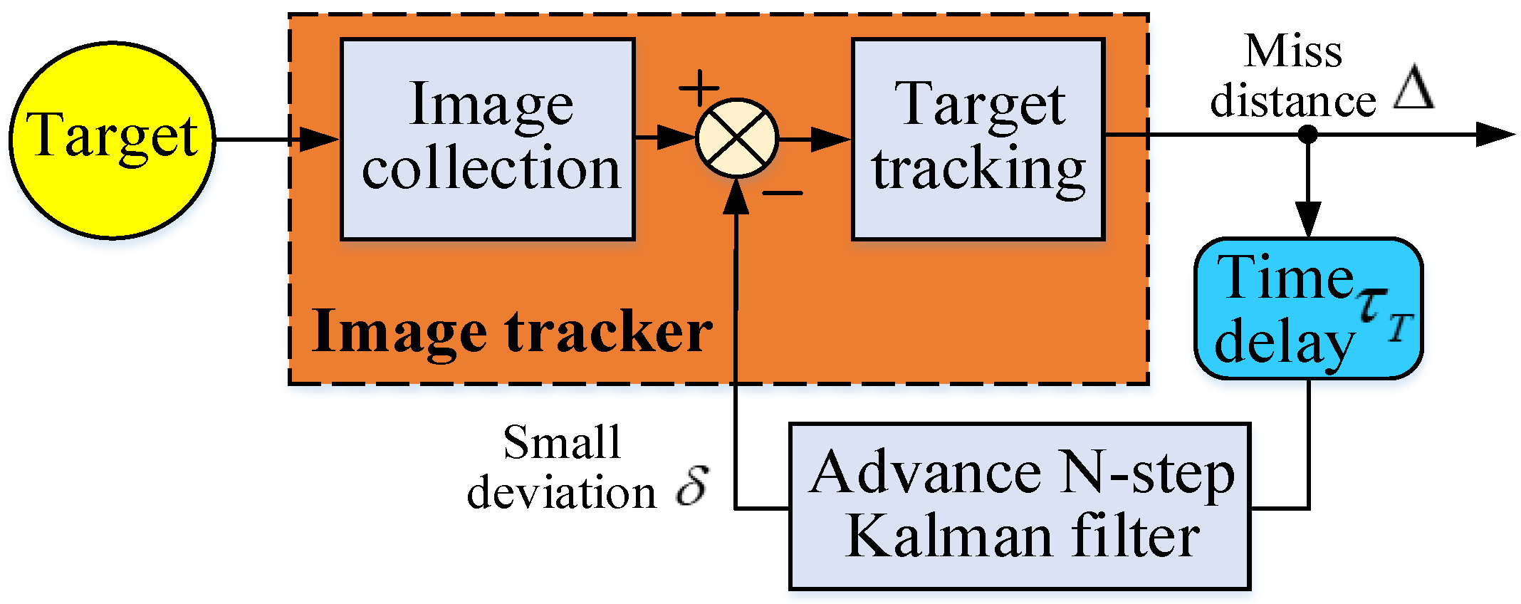
Figure 5 shows the optimized Kalman prediction filter of the EODS. The traditional signal fusion estimation field does not need too high precision. So it is usually limited to using an one-step prediction. However, for the practical applications in engineering fields such as tracking and aiming of EODS, the traditional filter should be improved.

The optimized model satisfies the following two assumptions.

Assumption 1.

State noise $W_k$ and observation noise $V_k$ are white noises with zero mean value and they are not related. Their variance is Q and R, respectively.

$$\left\{\begin{array}{l}E\left[W_k\right]=0,E\left[W_k{W}_j{}^{\mathrm{T}}\right]=Q_k{\delta }_{kj}\\ E\left[V_k\right]=0,E\left[V_k{V}_j{}^{\mathrm{T}}\right]=R_k{\delta }_{kj}\\ E\left[W_k{V}_j{}^{\mathrm{T}}\right]=0\end{array}\right.$$

(6)

In Equation (6), $\forall k,j$, ${\delta }_{kj}$ is the Kroneck function.

$${\delta }_{kj}=\left\{\begin{array}{l}1\hspace{1em}\left(k=j\right)\\ 0\hspace{1em}\left(k\ne j\right)\end{array}\right.$$

(7)

Assumption 2.

The initial value $x_0$ is not related to state noise $W_k$ and observation noise $V_k$.

$$\left\{\begin{array}{l}E\left(x_0\right)={\mu }_0\\ E\left[\left(x_0-{\mu }_0\right){\left(x_0-{\mu }_0\right)}^{\mathrm{T}}\right]=P_0\end{array}\right.$$

(8)

On the basis of Assumptions 1 and 2, and according to the last NT time estimated value, the current time-optimized equation can be deduced.

$${\widehat{X}}_{k|k-n}={\Phi }_{k|k-n}{\widehat{X}}_{k-n|k-n}+{\Gamma }_{k-n}{W}_{k-n}$$

(9)

Similarly, according to the last NT time mean square difference, the current time-prediction mean square error equation can be deduced.

$$P_{k|k-n}={\Phi }_{k|k-n}{P}_{k-n|k-n}{\Phi }_{k|k-n}^{\mathrm{T}}+{\Gamma }_{k|k-n}Q{\Gamma }_{k|k-n}^{\mathrm{T}}$$

(10)

The Kalman prediction gain matrix equation can be obtained.

$$K_k=P_{k|k-n}{H}_k^{\mathrm{T}}{\left[H_k{P}_{k|k-n}{H}_k^{\mathrm{T}}+R_k\right]}^{-1}$$

(11)

Then, using the data measured via the image tracker to correct the current state value, the current time-optimal prediction estimation equation can be deduced.

$${\widehat{X}}_{k|k}={\Phi }_{k|k-n}{\widehat{X}}_{k|k-n}+K_k\left[Y_k-H_k{\widehat{X}}_{k|k-n}\right]$$

(12)

Finally, the advanced N-step optimal filter prediction mean square error equation after data update can be deduced.

$$P_{k|k}={\left[P_{k|k-n}^{-1}+H_k^T{R}_k^{-1}{H}_k\right]}^{-1}$$

(13)

The EODS’s image tracker uses an optimal prediction filter structure based on the LOS’s linear motion transformation. So, the state transition matrix in Equation (5) can be deduced.

$${\Phi }_{k|k-n}=\left(\begin{array}{ccc}1& T& \raisebox{1ex}{$T^2$}\!\left/ \!\raisebox{-1ex}{$2$}\right.\\ 0& 1& T\\ 0& 0& 1\end{array}\right)$$

(14)

If the initial values $X_0$ and $P_0$ are known, the state estimation vector ${\widehat{X}}_{k|k}$ at time k can be calculated recursively according to the tracker observation value $Y_k$ at time k. If the observation value $Y_k$ has a time-delay τ, the actual observation value at time k is $Y_{k-n}$. Therefore, the current state estimate value ${\widehat{X}}_{k|k}$ at time k is actually the predicted LOS value $x_{k-n}$ at time k-n in the past.

The MD signal is different from the angular velocity signal of the incremental encoder, and the sampling period $T_{\mathrm{s}}$ of the encoder is generally in the range of 10 μs to 500 μs. And the change in period $T_{\mathrm{s}}$ is relatively small. The MD signal is affected by frame rate, lens resolution, and hardware computing power. Moreover, the sampling period $T_{\mathrm{k}}$ of the tracker is generally in the range of 1 ms to 100 ms. The longer the tracking time, the more exponential the increase in the amount of the algorithm running data. So this will lead to a phenomenon where the period $T_{\mathrm{k}}$ starts rapidly and then slows down. If the hardware performance is poor, the tracker will gradually deteriorate from MD time-delay to stagnation in the later stage. Therefore, compared with the speed loop incremental encoder, the MD signal of the position loop tracker can be regarded as a non-uniform sampling discrete signal.

By adjusting the step size n, the optimal Kalman algorithm suitable for different systems can be obtained. The parameters of this paper include a frame rate of 25 Hz and a lens resolution of 1280 × 720, with good hardware computing power. Based on the parameter configuration of the EODS, simulation was conducted using n = 3 as an example to demonstrate the effectiveness of the algorithm. According to the single-stage Kalman filter equation, the past state vector ${\widehat{X}}_{k|k-3}$ at time k − 3 is estimated from the current observation value $Y_{k-3}$ at time k. Then, ${\widehat{X}}_{k|k-3}$ is used to develop a three-step prediction to obtain the estimated LOS value ${\widehat{X}}_{k+3|k}$ at time k. Finally, the following mathematical equation is obtained.

$$\left\{\begin{array}{l}{\widehat{X}}_{k+3|k}={\Phi }_{k+3|k}{\widehat{X}}_{k|k}\\ {\widehat{Y}}_{k+3}=H_{k+3}{\widehat{X}}_{k+3|k}\end{array}\right.$$

(15)

According to the statistical results of the image tracker, the observation noise variance is R = 0.0019, and the time-delay is about ${\tau }_{\mathrm{T}}=40 \mathrm{ms}$. Suppose the filter initial value is $X_0={\left[0,0,0\right]}^{\mathrm{T}}$, the observation matrix is $H={\left[1,0,0\right]}^{\mathrm{T}}$, the mean square error of the initial value is $P_0=I_{3\times 3}$, and the filter gain matrix’s initial value is $K_0={\left[0,0,0\right]}^{\mathrm{T}}$. The model process noise Q is mainly obtained through comparative experiments.

$$Q=\left(\begin{array}{ccc}0& 0& 0.0002\\ 0& 0.0005& 0.0186\\ 0.0002& 0.0186& 0.9299\end{array}\right)$$

(16)

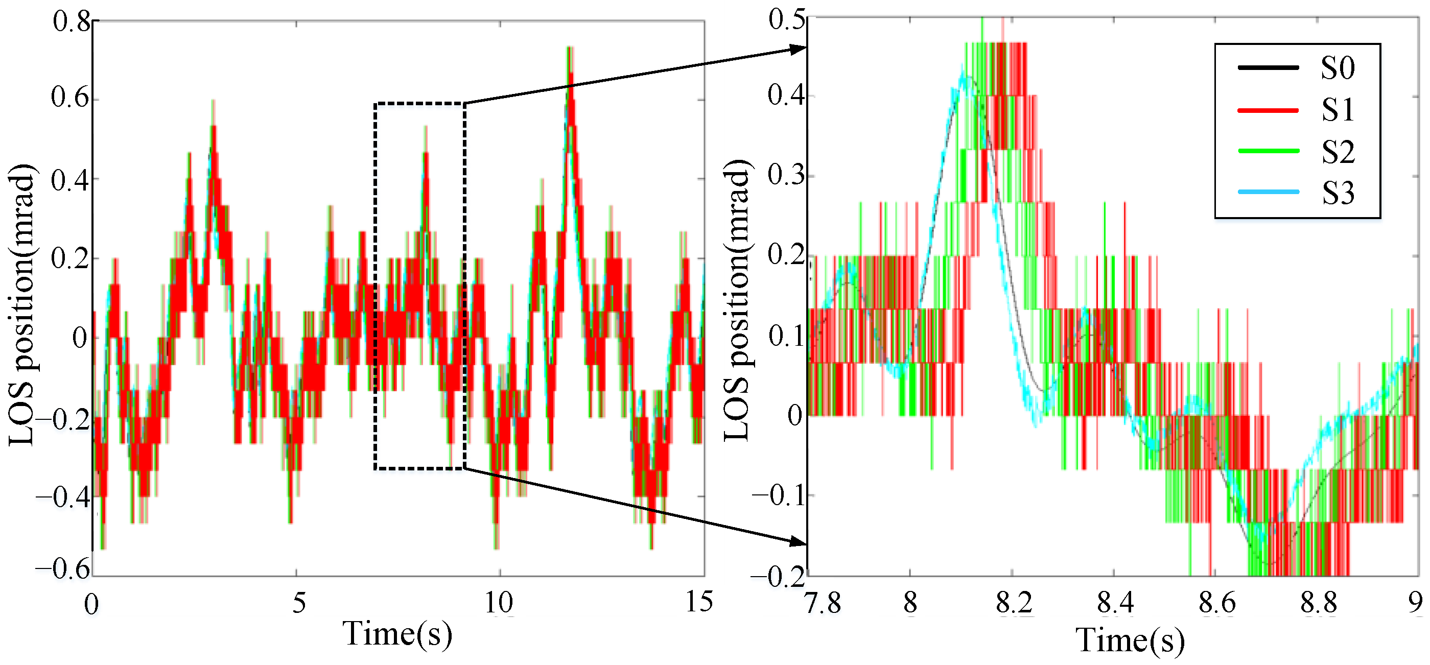
The model adopts the Runge Kutta fourth-order simulation, and the step length is set to 0.001 s. According to the linear motion transformation model, the LOS’s statistical data in the X azimuth direction are fitted as the frequency spectrum function. Then, the filter model inputs this function as the true value for testing. As shown in Figure 6, the black curve S0 represents the true value of the LOS. The red curve S1 represents the tracker measuring method. The green curve S2 represents the traditional moving-average filter method. The blue curve S3 represents the optimized design advanced N-step Kalman filter prediction method.

The black curve is set as the standard. In Figure 6, the red, green and blue curves have the same changing trend as the standard black curve. It shows that these methods can basically reflect the dynamic change in LOS’s true values. As shown in Figure 6, in the local expand area (7.8~9 s), the blue curve is closest to the black curve. It shows that the optimized method has the highest test accuracy compared with the other two groups.

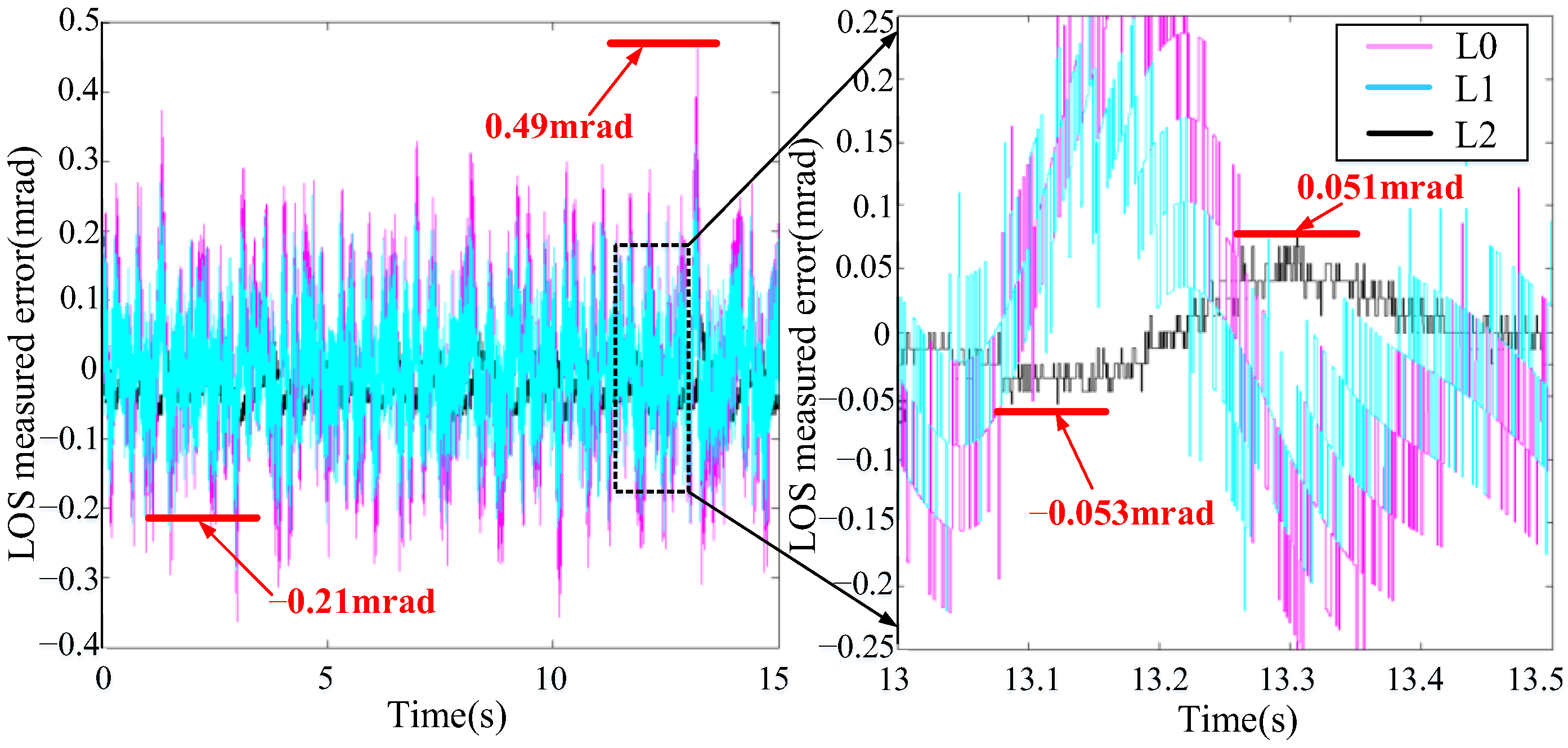
In Figure 7, the red curve L0 represents the inherent measured error between the image tracker’s measured value and the LOS’s true value. The blue curve L1 represents the traditional method’s measured error between the moving-average filtering value and the LOS’s true value. And the black curve L2 represents the optimal method’s measured error between the advanced N-step Kalman predicted value and the LOS’s true value.

In Figure 7, compared with the three curves, the red curve has the largest peak value, the black curve has the smallest peak value, and the blue curve is in the middle. Detailed data are shown in

Table 1. Comparison of tracking controller filter prediction error.

No	Index	Parameter
1	Inherent measured error of tracker δ1	0.49 mrad
2	Traditional method measured error δ2	0.21 mrad
3	Optimal method measured error δ3	0.053 mrad
4	Traditional method error ratio λ1 = 1 − δ2/δ1	57.1%
5	Optimal method error ratio λ2 = 1 − δ3/δ1	89.2%
6	Optimal/traditional method error ratio λ3 = 1 − δ3/δ2	74.8%

. The inherent measured error is 0.49 mrad (10~15 s), and the traditional method’s measured error is 0.21 mrad (0~5 s). So the traditional method’s error ratio is reduced by 57.1%. It shows that the traditional method can reduce the tracker’s inherent measured error to a certain extent. In Figure 7, in the local expand area (13~13.5 s), the black curve has two peaks. The upper bound of the black curve is 0.051 mrad, and the lower bound is −0.053 mrad. So the optimal method’s measured error is 0.053 mrad. The optimized method error ratio is reduced by 89.2%. It shows that both the traditional and optimal methods can reduce the tracker’s measured error. However, compared with the traditional method, the error correction effect of the optimal method is improved by 74.8%. It shows that the advanced N-step Kalman filter prediction controller can effectively correct the small deviation in the time-delay of a tracker and improve the shooting accuracy of an EODS.

3.2. Miss-Distance Judgment of LOS Firing Controller

The optimized filter controller can reduce the tracking time-delay error between the measured value and the true value. Then, it can output the accurate LOS predicted value. That is, the miss-distance Δ in Figure 8. To improve the tracking precision, it is also necessary to make the LOS’s predicted position coincide with the target’s actual position in the firing threshold value, so as to reduce the adverse impact of tracker time-delay error on EODS firing.

The time-delay of miss-distance Δ is about ${\tau }_{\mathrm{G}}=35 \mathrm{ms}$. The aiming and tracking actions of an EODS belong to a low frequency, small amplitude and a small range motion within 1.5 Hz. According to the linear motion transformation model, the mathematical equation of LOS firing control judgment correction can be obtained.

$$\left|X_s\left(t\right)\right|=\left|{\widehat{X}}_f\left(t\right)+{\omega }_g\left(t\right)\cdot {\tau }_{\mathrm{G}}\right|<{\Delta }_0$$

(17)

In Equation (17), ${\widehat{X}}_f\left(t\right)$ is the LOS’s predicted value. ${\tau }_{\mathrm{G}}$ is the time-delay. ${\omega }_{\mathrm{g}}\left(t\right)$ is the LOS’s angular velocity. ${\mathsf{\Delta }}_0$ is the firing judgment threshold. $X_s\left(t\right)$ is the LOS’s fusion value.

Ideally, when the LOS’s fusion value $X_s\left(t\right)$ coincides with the actual target position, $X_s\left(t\right)$ is the shooting accuracy ε. So the firing threshold value ${\Delta }_0$ should be less than ε. However, the actual manual tracking and aiming process is complex, and the LOS linear motion model will be affected by external factors. Therefore, a composite constraint Equation (18) is added based on the LOS judgment correction in Equation (17).

$$\left|{\widehat{X}}_f\left(t\right)\right|\le \frac{\epsilon }{2}$$

(18)

Combining Equations (17) and (18), a new mathematical equation can be obtained.

$$\left\{\begin{array}{l}\left|{\widehat{X}}_f\left(t\right)\right|<\frac{{\Delta }_0}{2}\le \frac{\epsilon }{2}\\ \left|X_s\left(t\right)\right|=\left|{\widehat{X}}_f\left(t\right)+{\omega }_{\mathrm{g}}\left(t\right)\cdot {\tau }_{\mathrm{G}}\right|<{\Delta }_0\le \epsilon \end{array}\right.$$

(19)

The lens resolution is N = 1280 × 720, and the lens field angle is $\beta$ = 3.6125° × 2.034°. When the number of pixels between the tracker’ measured value and the center of field view is n, the quantitative relationship of miss-distance Δ can be obtained.

$$\Delta =n\phi =\frac{n\beta }{N}$$

(20)

Then, the deviation value δ0 of a single pixel is converted to 0.0493 mrad using Equation (20). And the EODS needs to control the small deviation δ within 1~3 pixels in the lens of 1280 × 720 for long-distance precision shooting [6,7]. Suppose the small deviation δ caused by the tracker time-delay is n = ±3 pixels. So the tracker accuracy of X azimuth and Y pitch direction is ±0.14775 mrad and ±0.1479 mrad, respectively. The mathematical equation of preset accuracy ε can be obtained.

$$\epsilon =\mathsf{\Delta }=0.1479\approx 0.15 \mathrm{mrad}$$

(21)

As shown in Figure 9, the black curve P1 represents the LOS’s true value. The red curve P2 represents the LOS’s predicted value. The green curve P0 represents the LOS’s firing judgment threshold. The green curve represents the optimized design method proposed in this paper.

The black curve is set as the standard. In Figure 9, the green curve peaks three times in 0~15 s. It shows that the firing control judgment has been met for three times in this period. The third peak of the green curve occurs in 11.34~11.46 s. As shown in Figure 9, in the local expand area, the coincidence time of the LOS’s predicted value (red curve) and LOS’s true value (black curve) is 11.4 s. At this time, the LOS’s true value of the black curve is about 0.01 mrad, and the LOS’s predicted value of the red curve is about 0.03 mrad. It shows that the optimized method can effectively select the firing time.

As shown in

Table 2. Comparison of miss-distance judgment of LOS firing controller.

No	Index	Parameter
1	Deviation value of pixel unit δ0	0.0493 mrad
2	Actual LOS value x1 at coincidence	0.01 mrad
3	Predicted LOS value x2 at coincidence	0.03 mrad
4	Preset accuracy ε	0.15 mrad
5	Test accuracy b = |x1 − x2|	0.02 mrad
6	Error ratio μ = 1 − εb/ε	86.7%

, the test accuracy is 0.02 mrad. Compared with the preset accuracy of 0.15 mrad, the test accuracy is improved by 86.7%. It shows that the optimized method can control the tracker time-delay error within 1~3 pixels. The LOS firing time is effectively judged to identify the target in the field view center of the EODS lens, so as to improve the tracking precision.

3.3. Miss-Distance Anti-Occlusion Detection and Tracking Controller

The precondition for the correct implementation of an LOS firing controller model is that the image tracker stably outputs the miss-distance Δ signal. In Figure 10, the tracker time-delay can be compensated via filter prediction. However, once the miss-distance Δ is lost in the tracking and aiming process, the LOS firing controller cannot be implemented. This will lead to a decrease in the tracking precision of the EODS. As shown in Figure 10, the basic principle of the optimized image tracker is to obtain a resolution coordinate position DSST filter through image processing. Then, the DSST filter stably outputs the pixel coordinate position of the target in the next frame.

The DSST filter is used to extract the image blocks $f_1,f_2,\cdots ,f_n$ with gray level feature from the single-sample detection area with resolution M × N [19,20,21]. Then, the filter $h_{\mathrm{t}}$ is solved to obtain the gray level response value $g_1,g_2,\cdots ,g_n$ corresponding to each image block $f_1,f_2,\cdots ,f_n$. The Gaussian function is selected as the expected response function and marked as $g_i$. The function peak value is located in the center of the corresponding sample $f_i$. Finally, the mathematical equation of DSST filter $h_{\mathrm{t}}$ is obtained.

$$\sigma ={\displaystyle \sum _{i=1}^n{‖h_{\mathrm{t}}\ast f_i-g_i‖}^2=\frac{1}{MN}}{\displaystyle \sum _{i=1}^n{‖{\overline{H}}_t\cdot F_i-G_i‖}^2}$$

(22)

In Equation (22), ∗ represents convolution. σ is the minimum mean square error. $h_{\mathrm{t}},g_n,f_n$ are parameters extracted from the M × N detection area. f is the gray level feature of different image blocks from the previous frame. g is the response value constructed using the Gaussian function. h is the template updated by each iteration. The response values $g_1,g_2,\cdots ,g_n$ follow the Gaussian distribution and the response maximum $g_{\max }=g_i$ is located at the center of the corresponding gray level image block. $F_i,{\overline{H}}_{\mathrm{t}},G_i$ is the discrete Fourier transform corresponding to image block $f_n$, response value $g_n$, and DSST filter $h_{\mathrm{t}}$. The underline indicates the parameter complex conjugate. Then, the mathematical equation of Equation (23) can be obtained.

$$H_{\mathrm{t}}=\frac{{\displaystyle {\sum }_{i=1}^n{\overline{G}}_i{F}_i}}{{\displaystyle {\sum }_{i=1}^n{\overline{F}}_i{F}_i}}$$

(23)

In order to simplify and reduce the calculation amount of the DSST target tracker, the numerator and denominator of Equation (24) are recorded as $A_j$ and $B_j$ respectively.

$$\left\{\begin{array}{l}{A}_j=\left(1-\eta \right)A_{j-1}+\eta {\overline{G}}_j{F}_j\\ B_j=\left(1-\eta \right)B_{j-1}+\eta {\overline{F}}_j{F}_j\end{array}\right.$$

(24)

In Equation (24), η is the adjust coefficient, which represents the learning rate of the optimal filter. $A_j,B_j$ and $A_{j-1},B_{j-1}$ are the parameters of the current frame and the previous frame, respectively.

If the sample image Y resolution of the next frame is M × N, the updated response value Z can be obtained through Equation (25).

$$Z=F^{-1}\left\{\frac{{\displaystyle \sum \overline{A}Y}}{B+\lambda }\right\}$$

(25)

In Equation (25), $F^{-1}$ is the inverse discrete Fourier transform. λ is the adjust coefficient.

The area with the gray level response maximum is the target tracking position of the current frame. If the response value Z is the maximum $Z_{\max }$, the center point resolution coordinate ${\Delta }_{\mathrm{Z}}(x,y)$ of the corresponding image block is the new position for target tracking. The target coordinate ${\Delta }_{\mathrm{Z}}(x,y)$ is converted into miss-distance Δ, and stably output into the optimized prediction filter.

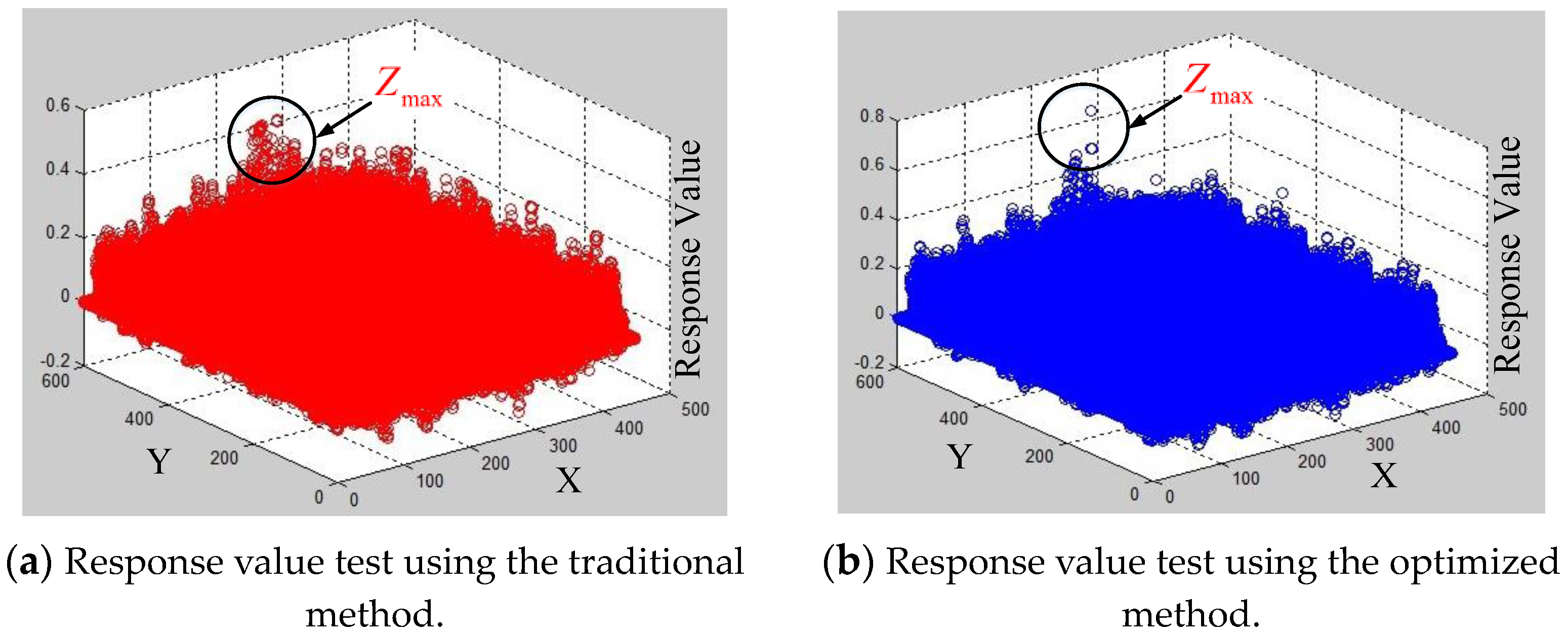
As shown in Figure 11a, an aerial view of the complex background is used as the single-sample training data of anti-occlusion DSST target tracking. Figure 12a,b shows the response value distribution comparison of two different methods. In Figure 12, the X-Y axes represent the resolution coordinates of the examination image. Z axis represents the response value distribution. There are multiple points in the black circle, but the highest point on the Z-axis is the response maximum $Z_{\max }$. Except for the maximum scatter, the more the interference scatters in the black circle, the more the occurrence of false detection. Compared with the traditional template matching method, the number of interference scatters of the optimized DSST tracking method is significantly decreased. The traditional method’s response maximum is 0.4, the optimized method’s response maximum is 0.7. Both of them can detect the cross target position. However, the response ratio of the optimized method increases by 42.9%. It shows that the target tracking stability of the optimized method is significantly improved and it can thus effectively avoid the target detection failure.

As shown in Figure 11a, an aerial view of the complex background is used as the single-sample training data for the anti-occlusion DSST target tracking. Figure 12a,b shows the response value distribution comparison of the two different methods. In Figure 12, the X-Y axes represent the resolution coordinates of the examination image. Z axis represents the response value distribution. The maximum scatter point in the black circle represents the response maximum $Z_{\max }$. Except for the maximum scatter, the more the interference scatters in the black circle, the more the occurrence of false detection. Compared with the traditional template matching method, the number of interference scatters of the optimized DSST tracking method is significantly decreased. The traditional method’s response maximum is 0.4, the optimized method’s response maximum is 0.7. Both of them can detect the cross-target position. However, the response ratio of the optimized method increases by 42.9%. It shows that the target tracking stability of the optimized method is significantly improved and it can thus effectively avoid the target detection failure.

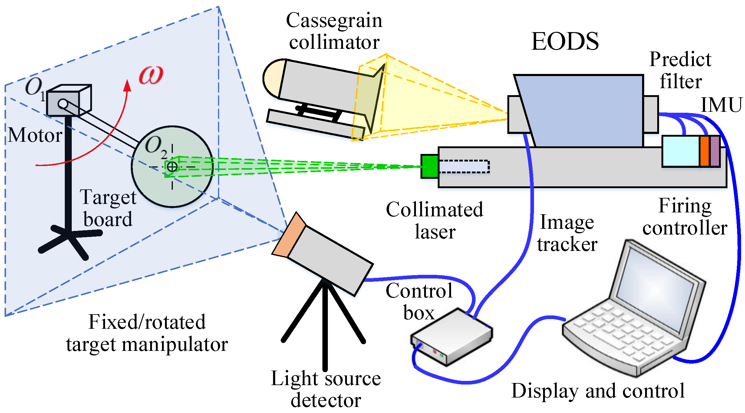
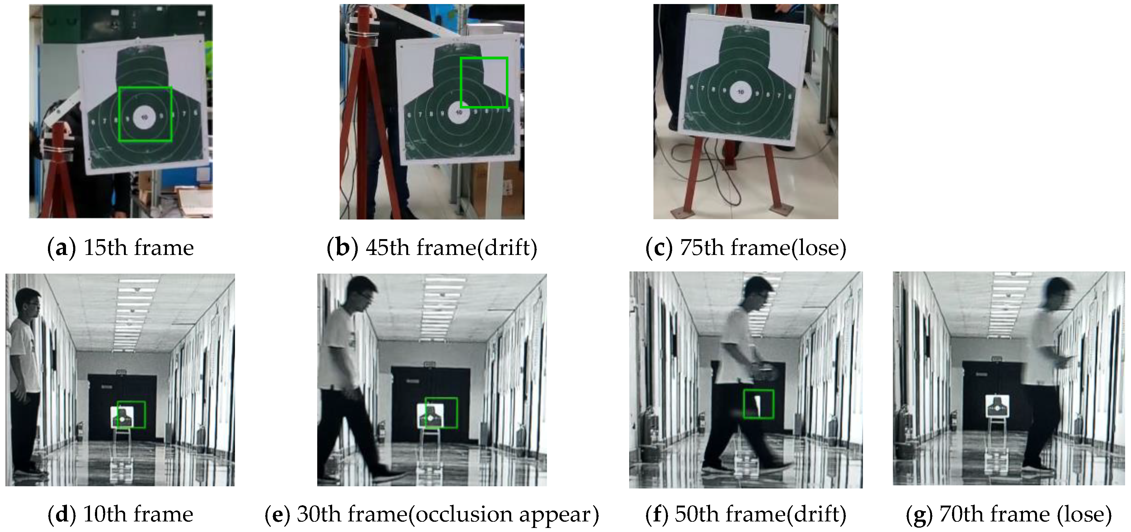
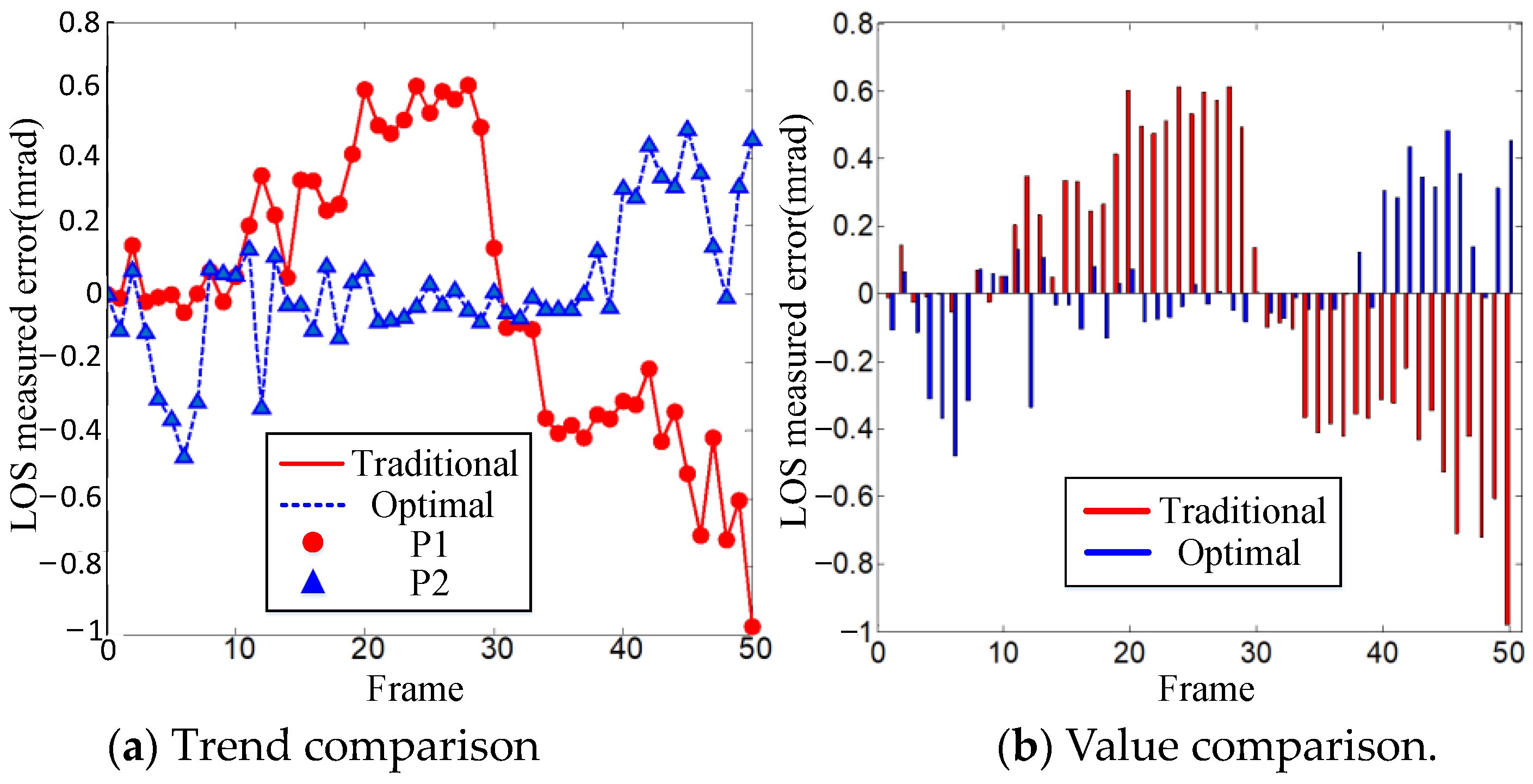
Figure 11b displays a target manipulator. As shown in Figure 2 and Figure 11b, the length of the connecting rod $O_1{O}_2$ is 70 cm. The target board rotates clockwise at an angular speed of 10°/s. Figure 13 and Figure 14 show the target tracking test results of the four groups of image sequences. The tracking distance of the rotated target is 50 m. The moving speed of the occlusion object is about 1.2 m/s. The tracking distance of the occluded target is 100 m.

In Figure 13a–c and Figure 14a–c, the traditional method causes a tracking drift error at the 45th frame and completely loses the target at the 75th frame. Compared with the traditional method, the optimized method can accurately and stably track the target’s motion. In Figure 13d–g and Figure 14d–g, compared with the traditional method, the optimized method can resist target occlusion. At the 30th frame, the occlusion object appears from the left. The traditional method causes a tracking drift error at the 50th frame and completely loses the target at the 70th frame. It shows that the anti-occlusion DSST tracking method can stably output the miss-distance Δ and improve the tracking precision.

4. Experimental Verification

The purpose of this experiment is to analyze the prediction and control mechanisms of the research object, which is an EODS. The LOS’s shooting accuracy is the core index. Experimental composition: an EODS, a Cassegrain collimator, Hikvision light source detector, collimated laser, precision rotating platform, and X-Y precision rotation actuator platform. Figure 15 shows the EODS’s experimental setup.

Table 3. Parameters of LOS’s tracking precision test.

No	Index	Parameter
1	Field angle of light source detector $\alpha \times \beta$	44.9° × 33.9°
2	Resolution of light source detector E × F	2592 × 2048
3	Frame frequency of light source detector K	19 Hz
4	Focal length of collimator objective lens F	1000 mm
5	Aperture of collimator d	140 mm

presents the performance parameters.

(1)

The traditional method is set as the control without adding filter prediction, and the image tracker utilizes a template matching method.

(2)

The optimal method is set as the test object with the addition of the advanced N-step Kalman filter prediction and LOS coinciding judgment correction systems. The image tracker uses an anti-occlusion DSST target tracking method.

The manual aiming and tracking action belong to a low frequency, small amplitude and a small range motion within 1.5 Hz. Moreover, the frequency–amplitude of pitch and azimuth direction are basically similar. According to the linear motion transformation model, it is supposed that the motion of the LOS in X and Y direction is the same. A Cassegrain collimator with the reticle is provided to simulate the infinity target. Then, the precision rotating platform is operated to test the LOS’s tracking precision in the X azimuth direction. The light source detector collects the laser offset data on the target board within 0~50 frames (about 3 s).

As shown in Figure 16, the trend of the LOS and the value of the two methods are compared through different manifestations of the same data. Figure 16a shows the line statistical chart. The red solid line represnts the measured error of the LOS via the traditional method, and the blue dotted line represents the error measured via the optimal method. Figure 16b shows the bar stacking chart. The red and blue areas represents the traditional method and the optimal method, respectively. The red curve is the control group. In Figure 16a, the blue curve has the same changing trend as the standard red curve. It shows that the optimized method can basically reflect the dynamic change in LOS’s position. However, compared with the red curve, the blue curve is closest to the Y = 0 mrad. It shows that the optimized method has a higher test accuracy.

As shown in Figure 16b, the LOS’s measured error, represented by the red area, via the traditional method is about −0.98 mrad (in 40~50 frame), and the error measured via the optimized method, represented by the blue area, is about −0.52 mrad (in 0~10 frame). Compared with the red area, the error of the blue curve is reduced by 46.9%. The EODS needs to control the small deviation within 1~3 pixels with the lens of 1280 × 720 for long-distance precision shooting [6,7,8,9]. According to the calculation of the lens field angle 3.6125° × 2.034° and Equations (20) and (21), the LOS’s preset accuracy should be within a circle with a radius of 0.15 mrad. As shown in

Table 4. LOS’s tracking test data via the traditional method.

Frame	LOS (mrad)	Frame	LOS (mrad)	Frame	LOS (mrad)	Frame	LOS (mrad)
0	0	13	0.233436	26	0.596136	39	−0.366864
1	−0.011064	14	0.049536	27	0.573036	40	−0.313164
2	0.142236	15	0.335736	28	0.613236	41	−0.324864
3	−0.023664	16	0.331836	29	0.491436	42	−0.219864
4	−0.009864	17	0.246636	30	0.135636	43	−0.433764
5	−0.001764	18	0.263736	31	−0.097764	44	−0.345264
6	−0.053064	19	0.411336	32	−0.085464	45	−0.528864
7	0.002436	20	0.600936	33	−0.104364	46	−0.708264
8	0.067236	21	0.495336	34	−0.365364	47	−0.421464
9	−0.023364	22	0.473136	35	−0.409164	48	−0.722964
10	0.052236	23	0.510936	36	−0.386064	49	−0.607464
11	0.202236	24	0.612036	37	−0.422964	50	−0.978864
12	0.347436	25	0.531636	38	−0.353964

and

Table 5. LOS’s tracking test data via the optimized method.

Frame	LOS (mrad)	Frame	LOS (mrad)	Frame	LOS (mrad)	Frame	LOS (mrad)
0	0	13	0.108384	26	−0.032316	39	−0.039516
1	−0.107316	14	−0.032616	27	0.008484	40	0.308184
2	0.066684	15	−0.032916	28	−0.049116	41	0.283884
3	−0.113616	16	−0.106416	29	−0.081816	42	0.435984
4	−0.310416	17	0.080184	30	0.003984	43	0.343584
5	−0.368616	18	−0.131016	31	−0.056916	44	0.315384
6	−0.479616	19	0.031584	32	−0.073416	45	0.481884
7	−0.318516	20	0.070584	33	−0.011316	46	0.354984
8	0.072084	21	−0.083016	34	−0.046416	47	0.139284
9	0.059484	22	−0.076716	35	−0.045516	48	−0.012816
10	0.053784	23	−0.070116	36	−0.045516	49	0.314184
11	0.130284	24	−0.038616	37	−0.000816	50	0.455184
12	−0.335016	25	0.027684	38	0.124284

, the optimized method’s distribution probability of the LOS’s measured error in the circle with a radius of 0.15 mrad is 72%, and the traditional method’s is 30%. In

Table 6. Comparison of LOS’s tracking test accuracy.

No	Index	Parameter
1	Tracking accuracy f	≤0.15 mrad
2	Actual physical significance of tracking accuracy f	Within 1~3 pixels
3	Traditional method 0.15 mrad intra-circle probability Q1	30%
4	Optimal method 0.15 mrad intra-circle probability Q2	72%
5	Tracking accuracy ratio K = 1 − Q1/Q2	58.3%

, compared with the traditional method, the LOS’s shooting accuracy using the optimized method is improved by 58.3%. It shows that the optimized method can reduce the adverse effect of a tracker time-delay error on EODS and significantly improve the LOS tracking precision.

5. Conclusions

This paper presents a new method for the prediction and control of small deviation in the time-delay of the tracker in an intelligent EODS. A miss-distance advanced Kalman prediction filtering controller is designed, the miss-distance judgment of the LOS firing controller is established, and a miss-distance anti-occlusion detection and tracking controller is used. The test shows that the distribution probability of the LOS’s measured error in a circle with a radius of 0.15 mrad is 72%. Compared with the traditional method, the LOS’s tracking precision using the optimized method is improved by 58.3%.

In conclusion, the new prediction and control method presented in this paper can effectively reduce the adverse impacts of small deviation in the tracker time-delay to improve the tracking precision and shooting accuracy of an EODS.