Design of a Noncontact Torsion Testing Device Using Magnetic Levitation Mechanism

Abstract

To facilitate torsion testing in special environments, a noncontact torsion testing device, where a noncontact torque can be transmitted to a specimen, was developed using magnetic levitation technology. A permanent magnetic gear is used to produce noncontact torque. In addition, four electromagnets and four attractive-type permanent magnetic bearings were employed to realize levitation; in more detail, the four electromagnets actively stabilized two levitation degrees of freedom (DoFs), while the four attractive-type permanent magnetic bearings passively stabilized four DoFs. Furthermore, a plant model considering the effect caused by the four attractive-type permanent magnetic bearings was built for the two levitation DoFs requiring active control. Based on the plant model, two PD-controllers were designed. Moreover, a control simulation was conducted to obtain appropriate PD-gains. Finally, experiments further validated the feasibility of the whole scheme, and it was proven that the device can apply a 0.126 N·m torque to the specimen while maintaining levitation.

1. Introduction

Magnetic levitation (Maglev) technology has aroused extensive attention due to its advantages of being friction-free, lubrication-free, and maintenance-free, and it has been used in many industrial applications, such as railway systems [1,2,3,4,5,6], rotating machinery [7,8,9,10,11,12], ultra-clean assembly line, and artificial heart pumps [13,14], which are the typical applications of maglev. In addition to these, there are some novel applications of maglev, such as maglev gyro [15], maglev globe [16], maglev lateral vibration attenuation system [17], permanent maglev system [18,19], and zero-power maglev system [20,21]. Similarly, in our previous research, to cater to the testing requirements for the parts and materials working in special environments, we applied maglev to tension and bending testing devices [22,23]. Special environments include vacuum, special gases, and special liquids, as well as environments with abnormal air pressure or temperature, which may greatly influence the mechanical performance of the parts or components; therefore, it is necessary to facilitate the mechanical test in special environments. E.g., high-purity aluminum [24], which is widely used in satellites, spacecraft, and other aerospace devices, has to work in vacuum environments because, in normal air, a layer of oxide film will form on its surface, impairing its mechanical performance, corrosion resistance, and adhesion. In addition, gas-lubricated bearings [25] need to work in helium environments to reduce air resistance and better heat dissipation during high-speed rotation because helium has a lower viscosity and higher thermal conductivity compared with ordinary air. Furthermore, silicon-based photonic chips [26], which are typically used in optical communication and sensing, need to work in nitrogen environments because nitrogen can help silicon-based photonic chips maintain optical performance and stability. Previously, if we wanted to test these parts or materials’ mechanical properties in their original working environment, the entire material testing device had to be placed in a container in which the special environment was. On the contrary, with maglev technology, the specimens in the devices [22,23] can be applied with load in a noncontact way; as a result, only the specimens and a few parts need to be placed in the container where the special environment can be created, which avoids exposing sensitive components of the testing device (e.g., circuits in force sensors and actuators are sensitive to environment humidity) to the special environment, facilitating the conduct of the testing. The research [22,23] was inspired by the research [27] held by Okayama University. In the research [27], Naoya Tada and Hiroyasu Masago developed a device in which a noncontact tension force can be applied to one end of a specimen using permanent magnets. As the tension force can be transmitted to the specimen in a noncontact way, the specimen can be isolated from the fixture at the end, and the specimen can be put in a container where a liquid environment can be created, which will be helpful to liquid and humid environment’s testing. However, the device in the research [27] only allows one end of the specimen to realize noncontact force; the other end still remains in contact force. Therefore, it is difficult to seal the specimen in a closed container, but a completely closed container is necessary to create a vacuum and gas environment. That is to say, this device is only helpful for testing in a liquid environment and not really helpful for testing in a gas or vacuum environment. To address this issue, in the research [22,23], we developed a completely noncontact tension testing device and a completely noncontact bending device using maglev technology. In addition, by designing various maglev mechanisms, various types of noncontact material testing devices can be developed. The Torsion test is one of the most common mechanical tests; it can directly measure the shear strength of materials, which is a very important parameter in some applications. The Torsion test is applicable to a wide variety of materials, such as metals, polymers, ceramics, and composites, and it is a short test that can usually be finished in a few minutes. Due to these advantages, it is widely used in metal processing, material research, medical equipment, and the automobile industry. Given the status and superiority of the Torsion test, in this paper, we focus on developing a noncontact torsion testing device using maglev technology.

Primarily, it is necessary to consider a control scheme for global levitation stability. Generally, there are six levitation degrees of freedom (DoF) for a rigid levitated object. If many levitation DoFs can be inherently stable, i.e., passively stable, a lot of hardware, such as displacement sensors, electromagnets, amplifiers, and controllers can be saved. Therefore, we want the designed structure to have as many passively stable levitation DoFs as possible. However, according to Earnshaw’s theorem [28], it is necessary that at least one levitation DoF be actively controlled for complete non-contact. In this paper, to maximize passively stable levitation DoFs, a structure with four passively stable levitation DoFs was designed. In the structure, the passive stability is mainly realized by four attractive-type permanent magnetic bearings; each attractive-type permanent magnetic bearing consists of two axially magnetized permanent magnet rings. Furthermore, to produce noncontact torque, we employed one permanent magnetic gear, which consists of two radially magnetized permanent magnets.

Furthermore, there are still two levitation DoFs to be actively controlled. We used typical attraction-type electromagnetic levitation for these two DoFs. Generally, a PD-controller is enough for ordinary electromagnetic levitation, and PD-gains are usually determined based on the plant model derived from the electromagnetic force model. However, in this case, since the attractive-type permanent magnetic bearings are involved in the work, the plant model will be affected by the permanent magnetic force. To obtain proper PD-gains, it is necessary to consider the effect caused by the permanent magnetic force. Therefore, before building the plant model, FEM analysis was conducted on the attractive-type permanent magnetic bearings to obtain their support characteristics. Then, taking the support characteristics into account, a plant model was built. With the plant model, two PD-controllers were designed.

This paper is organized as follows: Section 1 is the research background. Section 2 describes the structure and the working principle of the device. Section 3 is about the control of the two DoFs, including the plant model building process, the PD-controller design process, and simulation verification. Section 4 conducts an experiment to verify the feasibility of the device. Section 5 draws a summary and extension of this paper.

2. Structure and Working Principle

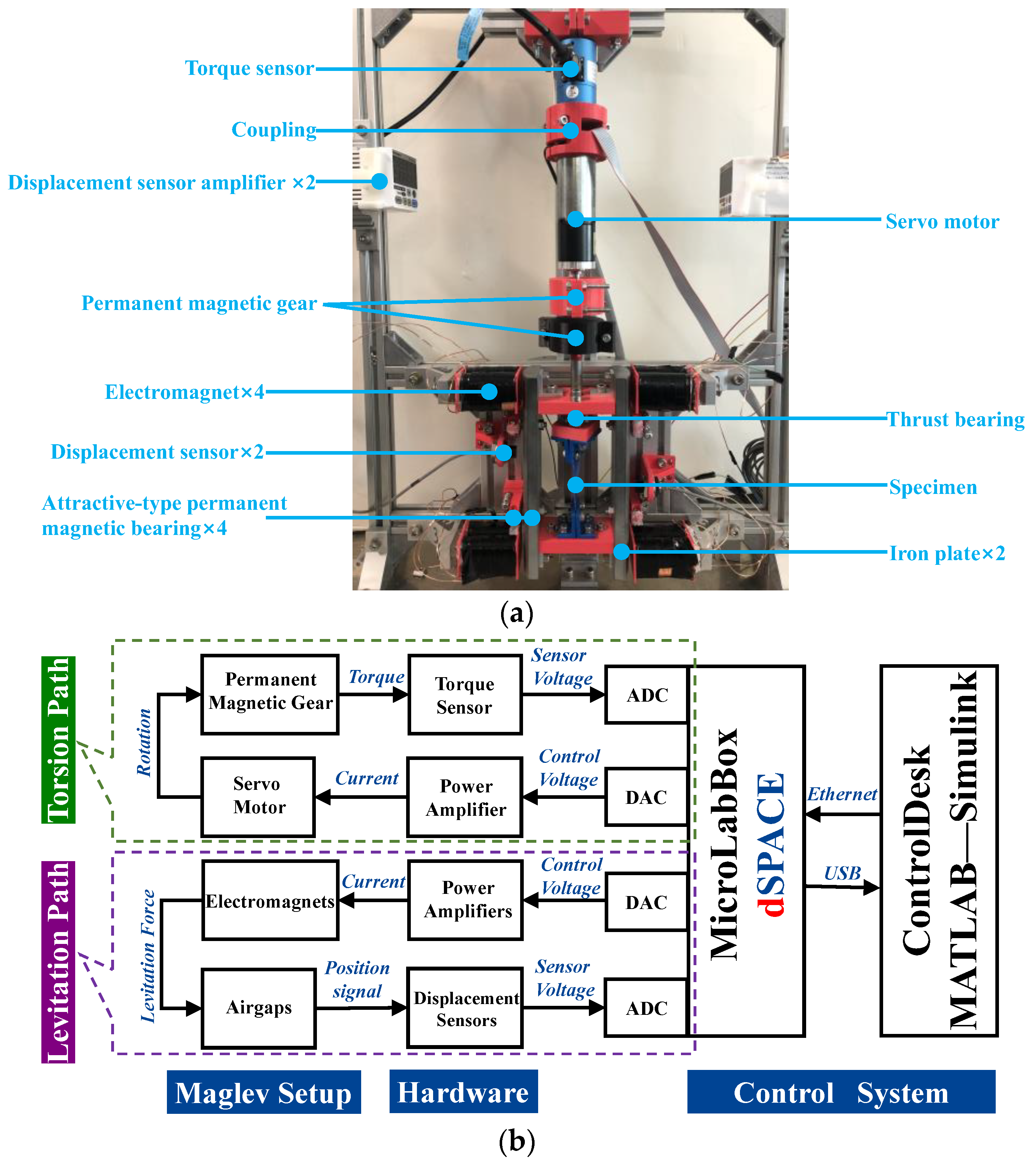
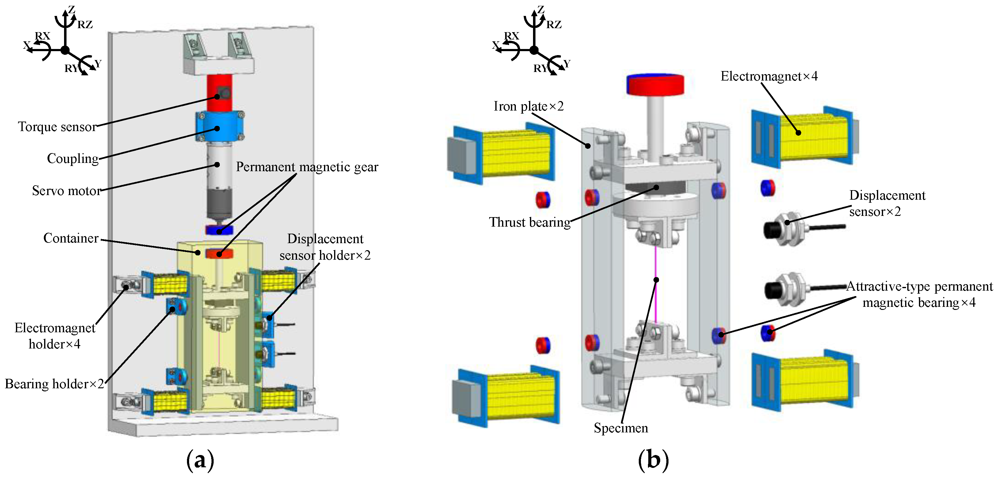
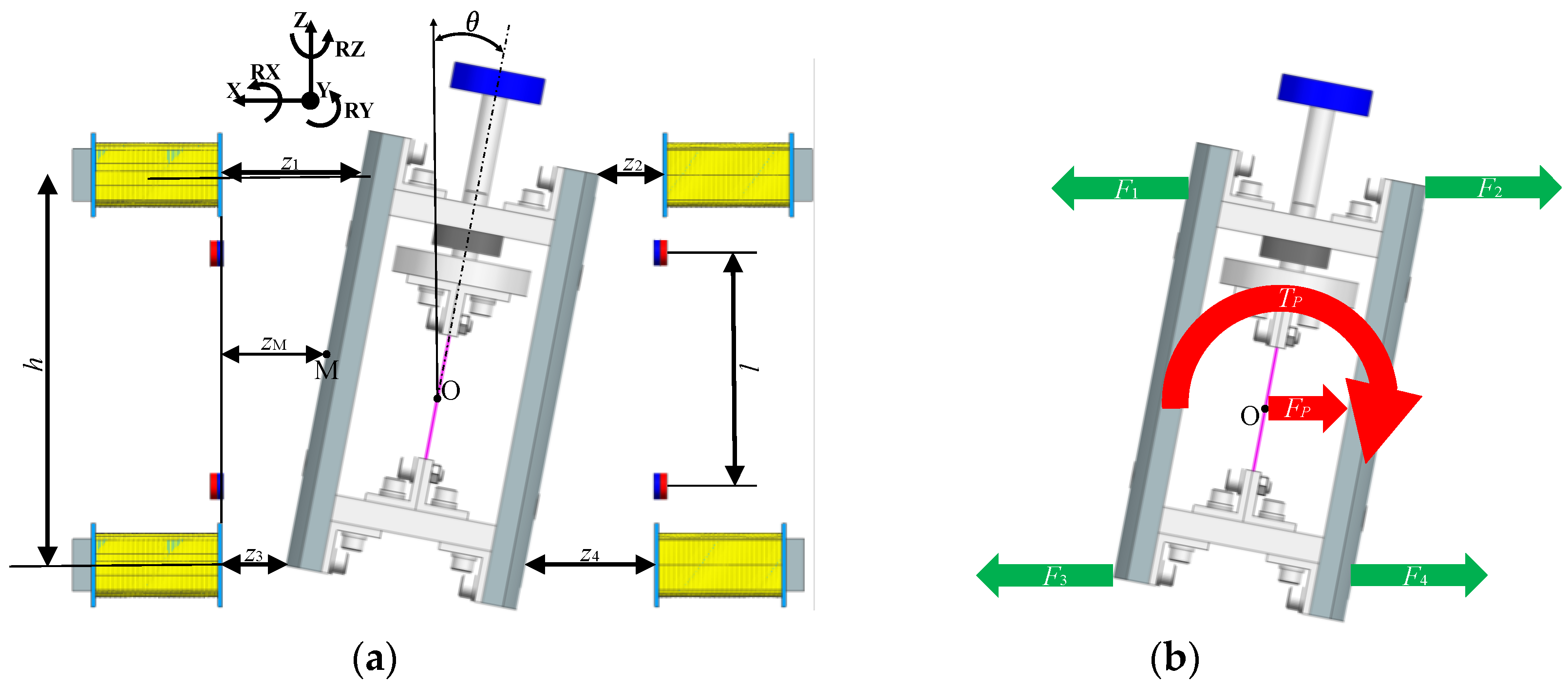
2.1. Structure Overview

Figure 1 gives a schematic diagram to highlight the advantages of this research. Figure 1a represents the traditional torsion testing mechanism, which applies contact torque to the specimen. As shown in Figure 1a, if a traditional torsion testing mechanism is used to test a specimen in a special environment (liquid, vacuum, or humid environment), since contact force is required, the whole device, including the torque sensor, actuator, etc., has to be put in a container where the special environment is created. In addition, as shown by the green line in Figure 1a, to provide support for the torque, both ends of the whole device have to be fixed to the inner wall of the container; that is to say, the container needs to bear the torque. However, on the one hand, the actuator and torque sensor contain circuits, which are sensitive to liquid, air humidity, or barometric pressure; on the other hand, since the container needs to bear the torque, the method is not applicable to the test in the soft body. As an improvement, the mechanism in Figure 1b not only employs noncontact torque using permanent magnetic gear, which prevents the actuator and torque sensor from entering the special environment, but also employs magnetic levitation to support the torque, which avoids the container bearing the torque.

Figure 2 gives two illustrations to describe the structure and the working principle. As shown in Figure 2a,b, a magnetic levitation torsion testing device (MLTTD) mainly consists of a torque sensor, a servo motor, a permanent magnetic gear made of two radially magnetized disc-shaped permanent magnets, four attractive-type permanent magnetic bearings each made of two axially magnetized annular permanent magnets, two displacement sensors, a specimen, two iron plates, a thrust bearing, and four electromagnets. The specification of the main components is shown in

Table 1. Specification of main components.

Name	Material/Model	Number
Torque sensor	Forsentek FT05	1
Servo motor	Maxon A-max 32	1
Displacement sensor	Panasonic GP-XC12ML	2
Permanent magnetic gear	N40	1
Attractive-type permanent magnetic bearing	N40	4

. As shown in Figure 2b, there is a semi-transparent container; the contents of the container are the levitated object, which includes one of the disc-shaped permanent magnets, the thrust bearing, the specimen, the iron plates, and half of the attractive-type permanent magnetic bearing pairs.

In brief, the permanent magnetic gear is used to generate noncontact torque, and the torque sensor is used to measure the noncontact torque; the four electromagnets and the four attractive-type permanent magnetic bearings are used to control levitation. Since there are two levitation DoFs that require active control, the two displacement sensors are equipped for active control.

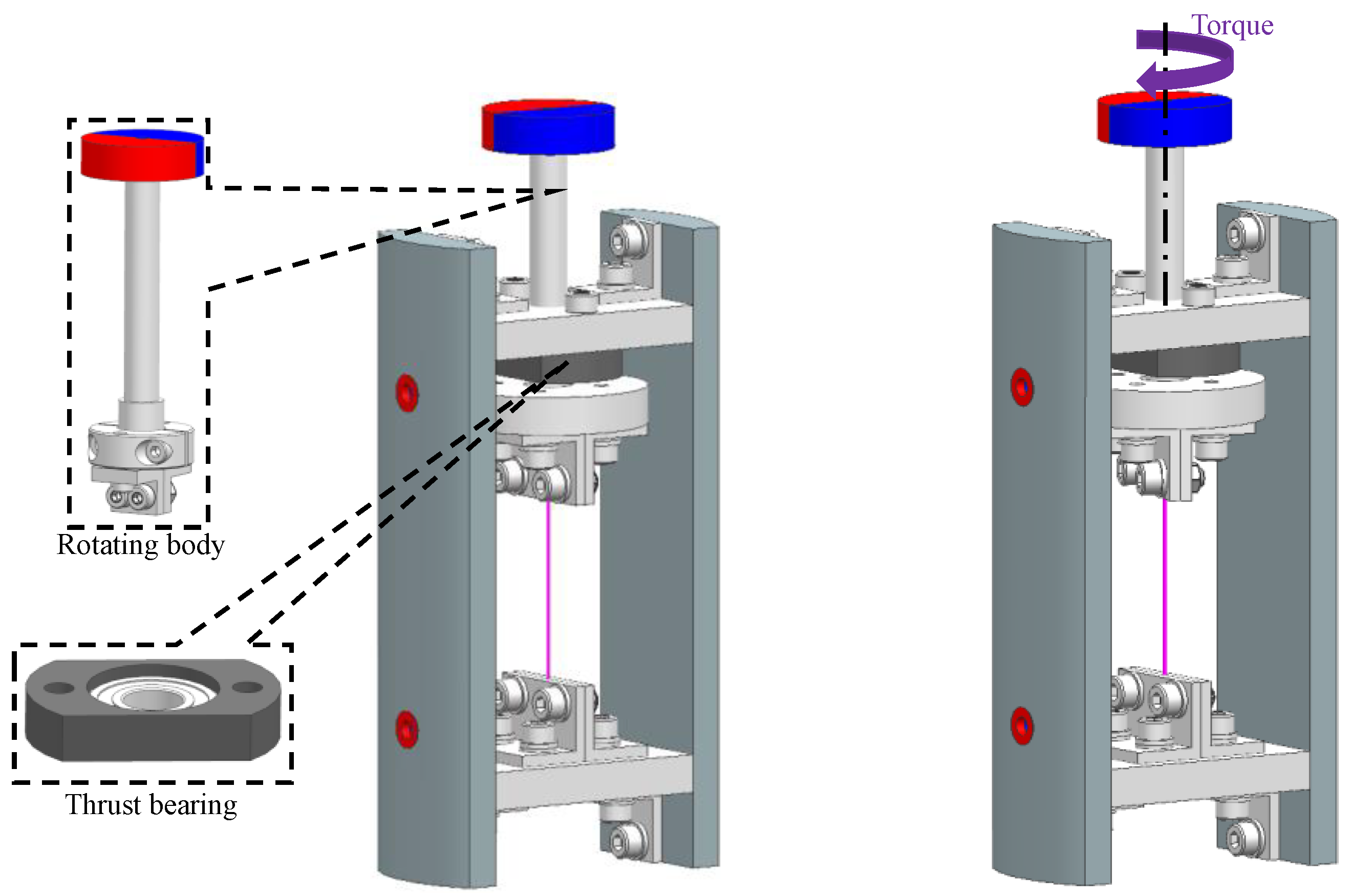
2.2. Principle of Levitation

Figure 3 presents an illustration to describe the six levitation DoFs, they are X, RX, Y, RY, Z, and RZ.

Table 2. Control strategy of the six levitation DoFs.

Degree of Freedom	Control Type	Component That Implements Control
X	Active	The four electromagnets
Y	Passive	The four attractive-type permanent magnetic bearings
Z	Passive	The four attractive-type permanent magnetic bearings
RX	Passive	The four attractive-type permanent magnetic bearings
RY	Active	The four electromagnets
RZ	Passive	The four attractive-type permanent magnetic bearings

shows the control strategy for the six levitation DoFs. As shown in Table 2, X and RY are actively controlled, while RX, Y, Z, and RZ are passively controlled. In more detail, referring to Figure 3 and Figure 2b, the two displacement sensors detect X and RY for feedback, the displacement data will be transmitted to a controller, and the controller will adjust the currents of the four electromagnets in real-time according to the displacement data so that the levitated object will be kept at a constant position in both the X-direction and the RY-direction. On the other hand, RX, Y, Z, and RZ are passively controlled by the four attractive-type permanent magnetic bearings; the principle is that, due to the edge effect, a magnetic force will be generated between two permanent magnets of each pair once they are not concentric, and this magnetic force will hinder the permanent magnets from misalignment.

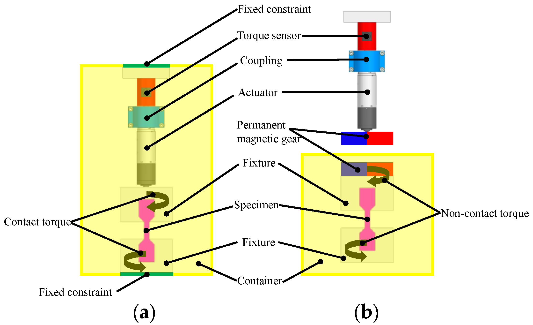
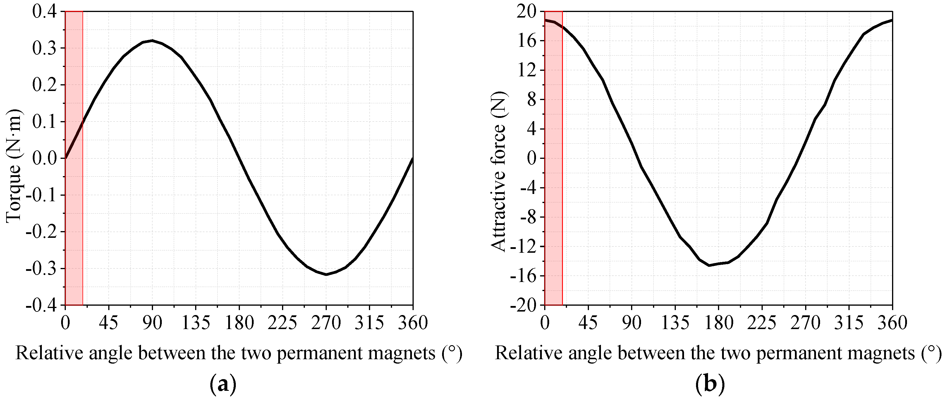
2.3. Principle of Torque Application

Figure 4 presents an illustration to describe the torque application. As described before, torque is generated by the permanent magnetic gear. As shown in Figure 2b, the upper permanent of the permanent magnetic gear is driven by a servo motor so that it can rotate; once it rotates, a noncontact torque will be generated for the other permanent magnet. As shown in Figure 4, driven by this torque, the rotating body will rotate, and through the thrust bearing, the rotation will be transmitted to the specimen so that the specimen can be twisted.

Figure 5 presents a FEM analysis result, which was calculated using J-mag software. In the analysis, the airgap between the two permanents was 17 mm. The abscissas of both graphs denote the relative angle between the two permanents; the ordinate of the first graph denotes the generated torque; and the ordinate of the second graph denotes the attractive force between the two permanents in the vertical direction. In this paper, we want to obtain 0.1 N·m torque. As shown by the red area in Figure 5a, as long as the relative angle reaches no more than 20°, 0.1 N·m torque can be obtained. On the other hand, as can be seen from the red area in Figure 5b, the attractive force will change from 18.8 N to about 17.7 N while the torque is increasing. The attractive force can be used to support the levitation in the Z-direction so that the burden of the attractive permanent magnetic bearings will be reduced and the attractive force will not be transmitted to the specimen because the thrust bearing will block any upward force. Although the attractive force will change a little during the torque application, it will be fine because the attractive-type permanent magnetic bearing will compensate for the change.

3. Control of X and RY

As mentioned in Section 2.2, X and RY require active control; therefore, this Section will discuss this issue.

3.1. Plant Model

3.1.1. State Space Model Derivation

To start, a plant model is built as follows: Figure 6 shows two illustrations for the plant model. In Figure 6a, z₁, z₂, z₃, and z₄ are the four airgaps between the electromagnets and the iron plates. O is the centroid of the levitated object. M is the point on the surface of the iron plate at the same vertical height as the midpoint of z₁ and z₂. Obviously, $z_M=\frac{z_1{+z}_3}{2}$. l is the vertical distance between the lower and upper attractive-type permanent magnetic bearings. h is the vertical distance between the lower and upper electromagnets. In Figure 6b, F₁, F₂, F₃, and F₄ denote the attractive forces of the four electromagnets on the iron plates, respectively. F_P and T_P, respectively denote the resultant force and resultant torque of the four attractive-type permanent magnetic bearings on the levitated object.

The expressions of F₁, F₂, F₃, and F₄ are shown in Equation (1), where a and c are two coefficients depending on the shape and dimensions of the electromagnets and the iron plates, and i₁, i₂, i₃, and i₄ are the currents of the four electromagnets, respectively. As shown in Equation (2), F₁, F₂, F₃, and F₄ can be linearized at a working point (i₀, z₀), where i₀ and z₀ are a constant current and a constant airgap, respectively. In Equation (2), F₀ denotes the magnetic force when the current and airgap are just i₀ and z₀, and $\mathsf{\Delta }{i}_1=i_1-i_0$, $\mathsf{\Delta }{i}_2=i_2-i_0,\mathsf{\Delta }{i}_3=i_3-i_0, \mathsf{\Delta }{i}_4=i_4-i_0, z_1=z_1-z_0$, $\mathsf{\Delta }{z}_2=z_2-z_0,\mathsf{\Delta }{z}_3=z_3-z_0, \mathsf{\Delta }{z}_4=z_4-z_0$, in addition, k_i and k_z are the current coefficient and airgap coefficient, respectively. Their expressions are shown in Equation (3), which was derived by calculating the derivative of the magnetic force (Any of F₁, F₂, F_3, and F₄) with respect to the current (Any of i₁, i₂, i_3, and i₄) and the airgap (Any of z₁, z₂, z_3, and z₄) at the working point (i₀, z₀).

$$\left\{\begin{array}{l}{F}_1=\frac{a{i}_1^2}{{(z_1+c)}^2}\\ F_2=\frac{a{i}_2^2}{{(z_2+c)}^2}\\ F_3=\frac{a{i}_3^2}{{(z_3+c)}^2}\\ F_4=\frac{a{i}_4^2}{{(z_4+c)}^2}\end{array}\right.$$

(1)

$$\left\{\begin{array}{l}{F}_1=F_0+k_i\cdot \mathsf{\Delta }{i}_1-k_z\cdot \mathsf{\Delta }{z}_1\\ F_2=F_0+k_i\cdot \mathsf{\Delta }{i}_2-k_z\cdot \mathsf{\Delta }{z}_2\\ F_3=F_0+k_i\cdot \mathsf{\Delta }{i}_3-k_z\cdot \mathsf{\Delta }{z}_3\\ F_4=F_0+k_i\cdot \mathsf{\Delta }{i}_4-k_z\cdot \mathsf{\Delta }{z}_4\end{array}\right.$$

(2)

$$\left\{\begin{array}{l}{k}_i=\frac{2a{i}_0}{{\left(z_0+c\right)}^2}\\ k_z=\frac{2a{i}_0^2}{{\left(z_0+c\right)}^3}\end{array}\right.$$

(3)

It can be assumed that the whole levitated object is a rigid body, and point M has the same horizontal displacement as point M, so its dynamics can be described by Equation (4), where m is the mass of the levitated object and J is the moment of inertial around its centroid. F_P and T_P can be regarded as two generalized forces with stiffness, so Equation (4) can be rewritten as Equation (5), where k_a and k_r are the stiffnesses of F_P and T_P, respectively.

$$\left\{\begin{array}{l}\left(F_1-F_2\right)+\left(F_3-F_4\right)-F_P=-m{\ddot{z}}_{COM}\\ \left[\left(F_1-F_2\right)-\left(F_3-F_4\right)\right]\times \frac{h}{2}-T_P=-J\ddot{\theta }\end{array}\right.$$

(4)

$$\left\{\begin{array}{l}\left(F_1-F_2\right)+\left(F_3-F_4\right)-k_a\left(z_{COM}-z_0\right)=-m{\ddot{z}}_{COM}\\ \left[\left(F_1-F_2\right)-\left(F_3-F_4\right)\right]\times \frac{h}{2}-k_r\theta =-J\ddot{\theta }\end{array}\right.$$

(5)

As mentioned before, $z_M\mathrm{equals}\frac{z_1{+z}_3}{2}$. Furthermore, if the variation range of θ is very small, it can be approximately regarded that $\theta \mathrm{equals}\frac{z_1{-z}_3}{h}$. Therefore, Equation (5) can be rewritten as Equation (6). Then, substituting $\mathsf{\Delta }{i}_1=i_1-i_0$, $\mathsf{\Delta }{i}_2=i_2-i_0,\mathsf{\Delta }{i}_3=i_3-i_0, \mathsf{\Delta }{i}_4=i_4-i_0, z_1=z_1-z_0$, $\mathsf{\Delta }{z}_2=z_2-z_0,\mathsf{\Delta }{z}_3=z_3-z_0, \mathsf{\Delta }{z}_4=z_4-z_0$ and Equation (2) into Equation (6), Equation (7) can be obtained.

$$\left\{\begin{array}{l}\left(F_1-F_2\right)+\left(F_3-F_4\right)-k_a\left(\frac{z_1+z_3}{2}-z_0\right)=-m\frac{{\ddot{z}}_1+{\ddot{z}}_3}{2}\\ \left[\left(F_1-F_2\right)-\left(F_3-F_4\right)\right]\times \frac{h}{2}-k_r\times \frac{z_1-z_3}{h}=-J\frac{{\ddot{z}}_1-{\ddot{z}}_3}{h}\end{array}\right.$$

(6)

$$\left\{\begin{array}{l}{k}_i\cdot \left[\left(\mathsf{\Delta }{i}_1-\mathsf{\Delta }{i}_2\right)+\left(\mathsf{\Delta }{i}_3-\mathsf{\Delta }{i}_4\right)\right]-k_z\cdot \left[\left(\mathsf{\Delta }{z}_1-\mathsf{\Delta }{z}_2\right)+\left(\mathsf{\Delta }{z}_3-\mathsf{\Delta }{z}_4\right)\right]-\frac{k_a}{2}\left(\mathsf{\Delta }{z}_1+\mathsf{\Delta }{z}_3\right)=-m\frac{\mathsf{\Delta }{\ddot{z}}_1+\mathsf{\Delta }{\ddot{z}}_3}{2}\\ \frac{h}{2}\cdot k_i\cdot \left[\left(\mathsf{\Delta }{i}_1-\mathsf{\Delta }{i}_2\right)-\left(\mathsf{\Delta }{i}_3-\mathsf{\Delta }{i}_4\right)\right]-\frac{h}{2}\cdot k_z\cdot \left[\left(\mathsf{\Delta }{z}_1-\mathsf{\Delta }{z}_2\right)-\left(\mathsf{\Delta }{z}_3-\mathsf{\Delta }{z}_4\right)\right]-\frac{k_r}{h}\left(\mathsf{\Delta }{z}_1-\mathsf{\Delta }{z}_3\right)=-J\frac{\mathsf{\Delta }{\ddot{z}}_1-\mathsf{\Delta }{\ddot{z}}_3}{h}\end{array}\right.$$

(7)

It can be seen from the geometric relationship that $\mathsf{\Delta }{z}_1=-\mathsf{\Delta }{z}_2,$ $\mathsf{\Delta }{z}_3=-\mathsf{\Delta }{z}_4$. In addition, since differential driving mode [29] is employed for the four EM in this paper, therefore $\mathsf{\Delta }{i}_1=-\mathsf{\Delta }{i}_2,$ $\mathsf{\Delta }{i}_3=-\mathsf{\Delta }{i}_4$. As a result, Equation (7) becomes Equation (8).

$$\left\{\begin{array}{l}2k_i\cdot \left(\mathsf{\Delta }{i}_1+\mathsf{\Delta }{i}_3\right)-2k_z\cdot \left(\mathsf{\Delta }{z}_1+\mathsf{\Delta }{z}_3\right)-\frac{k_a}{2}\left(\mathsf{\Delta }{z}_1+\mathsf{\Delta }{z}_3\right)=-m\frac{\mathsf{\Delta }{\ddot{z}}_1+\mathsf{\Delta }{\ddot{z}}_3}{2}\\ h\cdot k_i\cdot \left(\mathsf{\Delta }{i}_1-\mathsf{\Delta }{i}_3\right)-h\cdot k_z\cdot \left(\mathsf{\Delta }{z}_1-\mathsf{\Delta }{z}_3\right)-\frac{k_r}{h}\left(\mathsf{\Delta }{z}_1-\mathsf{\Delta }{z}_3\right)=-J\frac{\mathsf{\Delta }{\ddot{z}}_1-\mathsf{\Delta }{\ddot{z}}_3}{h}\end{array}\right.$$

(8)

Furthermore, defining $\mathsf{\Delta }{z}_{+}=\mathsf{\Delta }{z}_1+\mathsf{\Delta }{z}_3$, $\mathsf{\Delta }{z}_{-}=\mathsf{\Delta }{z}_1-\mathsf{\Delta }{z}_3$, $\mathsf{\Delta }{i}_{+}=\mathsf{\Delta }{i}_1+\mathsf{\Delta }{i}_3$, $\mathsf{\Delta }{i}_{-}=\mathsf{\Delta }{i}_1-\mathsf{\Delta }{i}_3$, Equation (8) can be rewritten as Equation (9).

$$\left\{\begin{array}{l}\frac{4k_i}{-m}\cdot \mathsf{\Delta }{i}_{+}+\frac{4k_z+k_a}{m}\cdot \mathsf{\Delta }{z}_{+}=\mathsf{\Delta }{\ddot{z}}_{+}\\ \frac{k_i{h}^2}{-J}\cdot \mathsf{\Delta }{i}_{-}+\frac{k_z{h}^2+k_r}{J}\cdot \mathsf{\Delta }{z}_{-}=\mathsf{\Delta }{\ddot{z}}_{-}\end{array}\right.$$

(9)

After that, define a state space as follows:

$$X=\left[\begin{array}{c}\mathsf{\Delta }{z}_{+}\\ \mathsf{\Delta }{\dot{z}}_{+}\\ \mathsf{\Delta }{z}_{-}\\ \mathsf{\Delta }{\dot{z}}_{-}\end{array}\right]$$

(10)

$$U=\left[\begin{array}{c}\mathsf{\Delta }{i}_{+}\\ \mathsf{\Delta }{i}_{-}\end{array}\right]$$

(11)

$$Y=\left[\begin{array}{l}\mathsf{\Delta }{z}_1\\ \mathsf{\Delta }{z}_3\end{array}\right]$$

(12)

$$\left\{\begin{array}{l}X=AX+BU\\ Y=CX\end{array}\right.$$

(13)

where X is the state variable, U is the input, Y is the output, and Equation (13) is the state space expression. From Equation (9), the expressions of A, B and C can be drawn as follows: So far, the plant model has been built.

$$A=\left[\begin{array}{cccc}0& 1& 0& 0\\ \frac{4k_z+k_a}{m}& 0& 0& 0\\ 0& 0& 0& 1\\ 0& 0& \frac{k_z{h}^2+k_r}{J}& 0\end{array}\right]$$

(14)

$$B=\left[\begin{array}{cc}0& 0\\ \frac{4k_i}{-m}& 0\\ 0& 0\\ 0& \frac{k_i{h}^2}{-J}\end{array}\right]$$

(15)

$$C=\left[\begin{array}{cccc}0.5& 0& 0.5& 0\\ 0.5& 0& -0.5& 0\end{array}\right]$$

(16)

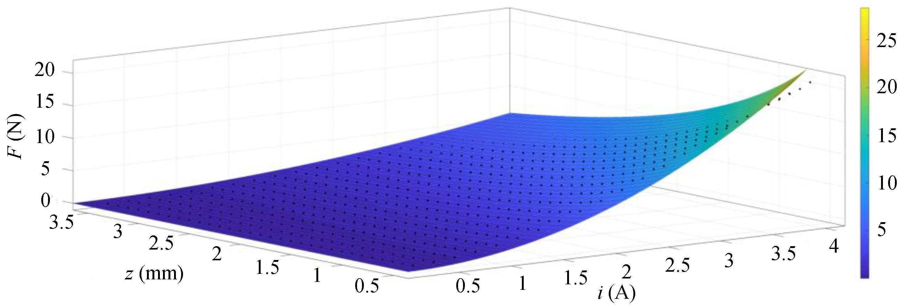
3.1.2. Determination of Plant Model Parameter

In Equations (14)–(16), there are some parameters to be determined; they are m, J, h, l, k_i, k_z, k_r, and k_a. Among them, m, J, h, and l can be easily calculated based on the densities, dimensions, and shapes of the solids; their values are 1.731 kg, 3.3 × 10⁻³ kg·m², 0.143 m, and 0.0774 m, respectively. k_i and k_z can be calculated using Equation (3), however, the calculation requires the values of a and c. Therefore, the attractive force of a single electromagnet to an iron plate was calculated at various combinations of current and airgap by FEM analysis. After the analysis, the result data were imported into the Curve Fitting Toolbox of MATLAB to obtain a fitting surface, which was generated in the form of $F=\frac{{\mathit{ai}}^2}{{(z+c)}^2}$, which is the general equation of electromagnetic force. The generated fitting surface is shown in Figure 7, where the black point is the original data. With the generation of the fitting surface, a and c were also calculated out by the toolbox; their values were 1.204 × 10⁻⁵ Nm² A⁻², 2.38 × 10⁻³ m, respectively. Furthermore, i₀ and z₀ were set as 2 A and 3 mm, and then k_i and k_z were calculated using Equation (3); their values were 1.6639 N/A and 618.5426 N/m, respectively.

Furthermore, to determine values for k_r and k_a, another FEM analysis was conducted on the four attractive-type permanent magnetic bearings. In the FEM analysis, the four permanent magnets in the bearing holder were set to be static, and the four permanent magnets embedded in the iron plate were set to be movable; then, F_P and T_P are calculated under various lateral displacements (z_M-z₀) and rotation angles (θ) of the four permanent magnets embedded in the iron plate. The results are shown in Figure 8. Figure 8a shows the result of F_P, and Figure 8b shows the result of T_P. It can be drawn from the slope of the red dashed line in both graphs that the stiffnesses k_a and k_r are approximately +12.5 N/mm and +0.133 N·m/° in the vicinity of the initial point (abscissa = 0). So far, all the plant model parameters have been caught, and the main parameter values are shown in

Table 3. Main parameters of the plant model.

Parameter Name	Parameter Value
a (Nm2A−2)	1.204 × 10−5
c (mm)	2.38
i0 (A)	2
z0 (mm)	3
ki (N/A)	1.6639
kz (N/m)	618.5426
m (kg)	1.731
J (kg·m2)	0.0033
h (m)	0.143
l (m)	0.0774

.

3.2. Control Design

As can be seen from Equation (14), the first two state variables and the last two state variables are not coupled to each other, therefore they can be controlled individually, so a feedback matrix with the following structure can be used:

$$K=\left[\begin{array}{cccc}{P}_1& D_1& 0& 0\\ 0& 0& P_2& D_2\end{array}\right]$$

(17)

where P₁, D₁, P₂, and D₂ can be regarded as two PD-gains of two independent PD-controllers. If the feedback matrix is used, a closed-loop system matrix will be as follows.

$$A+BK=\left[\begin{array}{cccc}0& 1& 0& 0\\ \frac{4k_z+k_a-4k_i{P}_1}{m}& \frac{-4k_i{D}_1}{m}& 0& 0\\ 0& 0& 0& 1\\ 0& 0& \frac{k_z{h}^2+k_r-k_i{h}^2{P}_2}{J}& \frac{-k_i{h}^2{D}_2}{J}\end{array}\right]$$

(18)

According to Equation (18), two independent characteristic equations can be derived as follows:

$$\left\{\begin{array}{l}{s}^2+\frac{4k_i{D}_1}{m}s+\frac{4k_i{P}_1-4k_z-k_a}{m}=0\\ s^2+\frac{k_i{h}^2{D}_2}{J}s+\frac{k_i{h}^2{P}_2-k_z{h}^2-k_r}{J}=0\end{array}\right.$$

(19)

$$\left\{\begin{array}{l}{s}^2+2{\zeta }_1{\omega }_{n1}\cdot s+{\omega }_{n1}^2=0\\ s^2+2{\zeta }_2{\omega }_{n2}\cdot s+{\omega }_{n2}^2=0\end{array}\right.$$

(20)

It can be seen from Equation (19) that they are two second-order systems. Generally, second-order systems have characteristic equations in the form of Equation (20), where ζ₁ and ζ₂ denote the damping ratios of the systems, ω_n1 and ω_n2 denote the undamped oscillation angular frequencies of the systems. Comparing Equations (19) and (20), the following equations can be derived.

$$\left\{\begin{array}{l}{\omega }_{n1}^2=\frac{4k_i{P}_1-4k_z-k_a}{m}\\ {\omega }_{n2}^2=\frac{k_i{h}^2{P}_2-k_z{h}^2-k_r}{J}\end{array}\right.$$

(21)

$$\left\{\begin{array}{l}2{\zeta }_1{\omega }_{n1}=\frac{4k_i{D}_1}{m}\\ 2{\zeta }_2{\omega }_{n2}=\frac{k_i{h}^2{D}_2}{J}\end{array}\right.$$

(22)

With Equations (21) and (22), the expressions of the PD-gains with respect to ζ₁, ζ₂, ω_n1, and ω_n2 can be obtained as follows:

$$\left\{\begin{array}{l}{P}_1=\frac{m{\omega }_{n1}^2+4k_z+k_a}{4k_i}\\ D_1=\frac{{\zeta }_1{\omega }_{n1}m}{2k_i}\end{array}\right.$$

(23)

$$\left\{\begin{array}{l}{P}_2=\frac{J{\omega }_{n2}^2+k_z{h}^2+k_r}{k_i{h}^2}\\ D_2=\frac{2{\zeta }_2{\omega }_{n2}J}{k_i{h}^2}\end{array}\right.$$

(24)

As can be seen from Equations (23) and (24), the PD-gains can be determined by determining the values of ζ₁, ζ₂, ω_n1, and ω_n2. In addition, damping ratio (ζ₁, ζ₂) and undamped oscillation angular frequency (ω_n1, ω_n2) determine the dynamic performance of the system. In more detail, as shown in Equations (25) and (26), damping ratio determines overshoot (M_p1, M_p2) of step response, while undamped oscillation angular frequency jointly determines settling time (t_s1, t_s2) of step response.

$$\left\{\begin{array}{l}{M}_{p1}=e^{\frac{-{\zeta }_1\pi }{\sqrt{1-{\zeta }_1{}^2}}}\times 100\%\\ t_{s1}\approx \frac{3}{{\omega }_{n1}{\zeta }_1}\left(5\%tolerance\right)\end{array}\right.$$

(25)

$$\left\{\begin{array}{l}{M}_{p2}=e^{\frac{-{\zeta }_2\pi }{\sqrt{1-{\zeta }_2^2}}}\times 100\%\\ t_{s2}\approx \frac{3}{{\omega }_{n2}{\zeta }_2}\left(5\%tolerance\right)\end{array}\right.$$

(26)

A damping ratio of 0.707 can coordinate overshoot and settling time; thus, it is usually regarded as an optimal damping ratio in practice [30]. Therefore, in this paper, 0.707 is taken for both ζ₁ and ζ₂. As a result, the overshoots will approach 4.33%. In addition, 0.025 s is taken for both t_s1 and t_s2, to realize that ω_n1 and ω_n2 should be 169.73 s⁻¹. Then, substituting ζ₁ = ζ₂ = 0.707 and ω_n1 = ω_n2 = 169.73 s⁻¹ into Equations (23) and (24), PD-gains that realize the desired dynamics performance will be obtained as

Table 4. The designed PD-gains.

Parameter Name	Parameter Value
P1 (A/m)	9886
D1 (A·s/m)	64
P2 (A/m)	3166
D2 (A·s/m)	23

.

3.3. Control Simulation

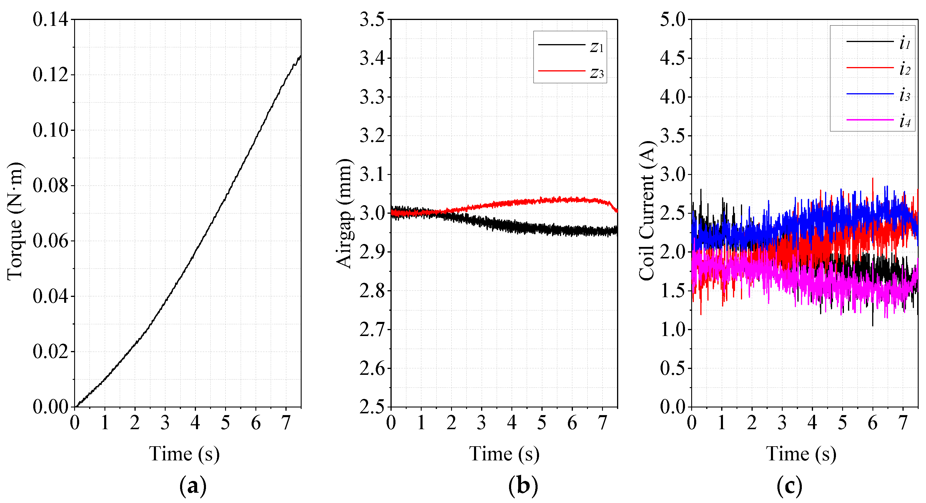
To verify the feasibility of the designed PD-controllers, control simulation was conducted using Matlab-Simulink. Control diagram is shown in Figure 9. The plant model parameters and control parameters in the simulation are the same as Table 3 and Table 4. To make the simulation closer to reality, the electromagnetic force model used in the simulation was the nonlinear plant model denoted by Equation (1) rather than the linearized plant model denoted by Equation (2). Moreover, to test the dynamic performance of the system, two sets of 0.1 mm step disturbances were applied to the airgaps at 0.1 s and 0.5 s, respectively; the first set was in the same direction, and the second set was in the opposite direction. The simulation result is shown in Figure 10.

As shown in Figure 10, after bearing the first step disturbance, the overshoots of both airgaps were about 3%, and the settling times (5% tolerance) of both airgaps were about 0.02 s. On the other hand, after bearing the second step disturbance, the overshoots of both airgaps were about 3%, and the settling times (5% tolerance) of both airgaps were about 0.02 s. This result implies that the dynamic performances in the simulation are slightly different from the designed dynamic performance (overshoot: 4.33%; settling time: 0.025 s); this may be due to the nonlinearity of the plant model used. Anyway, the overshoots (about 3%) of both responses were lower than the designed overshoot (4.33%), which implies the stability of the system is better than the design standard. On the other hand, the settling times (about 0.02 s) of both responses were shorter than the designed settling time (0.025 s), which implies the rapidity of the system is better than the design standard. To sum up, the designed PD-controllers are feasible.

4. Experiment

To validate the feasibility of the devices, an experiment was conducted. Figure 11a presents a photograph of the experiment setup, and Figure 11b presents an overall system structure diagram. The model of the torque sensor is FT05, made by FORSENTEK Co., Limited(Shenzhen, China); its measuring range is ±0.2 N·m. The model of the displacement sensors is GP-XC12ML, and the manufacturer is Panasonic Industry Co., Ltd. (Osaka, Japan). The power amplifiers are ESCON made by MAXON Japan Corp. (Tokyo, Japan). The control system is MicroLabBox dSPACE; it is equipped with software, i.e., ControlDesk. In ControlDesk, we can import a Matlab-Simulink file, adjust control parameters, record, and observe experiment data in real-time. In addition, as can be seen in Figure 11b, there are two paths, i.e., the levitation path and the torsion path; the former is used to stabilize X and RY, and the latter is used to apply noncontact torque. As mentioned before, the noncontact torque is generated by the relative rotation between the two disc-shaped permanent magnets; the rotation is driven by the servo motor. In the experiment, the servo motor drove the upper disc-shaped permanent magnet to rotate at a constant speed, so that a noncontact torque was generated on the lower disc-shaped permanent magnet, and through the thrust bearing, the torque was finally transmitted to the specimen.

Table 5. Control parameters in the experiment.

Parameter Name	Parameter Value
i0 (A)	2
z0 (mm)	3
P1 (A/m)	10,000
I1 (A/m/s)	1000
D1 (A·s/m)	50
P2 (A/m)	7000
I2 (A/m/s)	1000
D2 (A·s/m)	35

shows the control parameters in the experiments. Comparing Table 4 and Table 5, it can be found that the PD-gains in the experiment are a little different from the PD-gains in the simulation, but this is considered normal because the actual model and the theoretical model will inevitably deviate. In addition, as shown in Table 5, two integrators were added to the two PD-controllers, so that the two PD-controllers became two PID-controllers. Integrator can improve the robustness of the control system because, with the rotation of the permanent magnetic gear, the permanent magnetic gear will pose a disturbance and some uncertainty in the control of X and RY. Therefore, an integrator is added to deal with the disturbance and the uncertainty.

Table 6. Specification of the specimen.

Property Name	Property Value
Material	Z-ASA PRO
Length (mm)	67
Width (mm)	6
Thickness (mm)	1.6

shows the specifications of the specimen used in the experiment.

Figure 12 shows the experiment result, where Figure 12a shows torque data measured by the torque sensor and Figure 12b,c show airgap response and current response, respectively. As shown in Figure 12a, the torque kept increasing throughout the whole process; the maximum torque was about 0.126 N·m. As shown in Figure 12b, the two airgaps slightly fluctuated, but the airgap errors were within ±0.05 mm, which is considered fine.

5. Conclusions

To facilitate torsion testing in special environments, this paper proposes a noncontact torsion testing device using magnetic levitation technology, where a noncontact torque can be transmitted to a specimen. To ensure the stability of the six levitation degrees of freedom (DOF), four levitation DoFs are passively controlled by some permanent magnets, while two levitation DoFs are actively controlled by four electromagnets. Furthermore, a plant model was built for the control of the two levitation DoFs. With the plant model, two PD-controllers were designed, and the simulation result demonstrated that the designed PD-controllers make the system have good dynamic performance. Finally, an experiment was performed to test the stability of the levitation and the torque load capacity. The experiment result indicated that the device could apply a 0.126 N·m noncontact torque to the specimen while maintaining levitation.

Currently, the control mode of the torque is open-loop, which makes it impossible to accurately control the amount of torque. In the future, a torque feedback system will be constructed using torque sensors to apply the desired amount of torque.

References

1. Yougang, S.; Haiyan, Q.; Junqi, X.; Guobin, L. Internet of Things-based online condition monitor and improved adaptive fuzzy control for a medium-low-speed maglev train system. IEEE Trans. Ind. Inform. 2019, 16, 2629–2639. [Google Scholar]
2. Yonezu, T.; Watanabe, K.; Suzuki, E.; Sasakawa, T. Study on Electromagnetic Force Characteristics Acting on Levitation/Guidance Coils of a Superconducting Maglev Vehicle System. IEEE Trans. Magn. 2017, 53, 8300605. [Google Scholar] [CrossRef]
3. Tanaka, K. Impacts of the opening of the maglev railway on daily accessibility in Japan: A comparative analysis with that of the Shinkansen. J. Transp. Geogr. 2023, 106, 103512. [Google Scholar] [CrossRef]
4. Yuan, Y.; Li, J.; Deng, Z.; Liu, Z.; Wu, D.; Wang, L. Dynamic performance of HTS maglev and comparisons with another two types of high-speed railway vehicles. Cryogenics 2021, 117, 103321. [Google Scholar] [CrossRef]
5. Deng, Z.; Wang, L.; Li, H.; Li, J.; Wang, H.; Yu, J. Dynamic studies of the HTS maglev transit system. IEEE Trans. Appl. Supercond. 2021, 31, 3600805. [Google Scholar] [CrossRef]
6. Ke, H.; Lin, G.; Liu, Z. Prediction Approach of Negative Rail Potentials and Stray Currents in Medium-Low-Speed Maglev. IEEE Trans. Transp. Electrif. 2022, 8, 3801–3815. [Google Scholar]
7. Yamagishi, K. Optimum Design of Integrated Magnetic Bearing Using Multiple HTS Bulk Units. IEEE Trans. Appl. Supercond. 2019, 29, 6801505. [Google Scholar] [CrossRef]
8. Sugimoto, H.; Uemura, Y.; Chiba, A.; Rahman, M.A. Design of Homopolar Consequent-Pole Bearingless Motor with Wide Magnetic Gap. IEEE Trans. Magn. 2013, 49, 2315–2318. [Google Scholar] [CrossRef]
9. Liu, Z.; Chiba, A.; Irino, Y.; Nakazawa, Y. Optimum pole number combination of a buried permanent magnet bearingless motor and test results at an output of 60 kW with a speed of 37000 r/min. IEEE Open J. Ind. Appl. 2020, 1, 33–41. [Google Scholar] [CrossRef]
10. Cavalcante, R.G.; Fujii, Y.; Chiba, A. A bearingless motor with passive electrodynamic suspension in axial direction. IEEE Trans. Ind. Appl. 2021, 57, 6812–6822. [Google Scholar]
11. Hemenway, N.R.; Gjemdal, H.; Severson, E.L. New three-pole combined radial–axial magnetic bearing for industrial bearingless motor systems. IEEE Trans. Ind. Appl. 2021, 57, 6754–6764. [Google Scholar] [CrossRef]
12. Yunlei, J.; Torres, R.A.; Severson, E.L. Current regulation in parallel combined winding bearingless motors. IEEE Trans. Ind. Appl. 2019, 55, 4800–4810. [Google Scholar]
13. Samiappan, C.; Mirnateghi, N.; Paden, B.E.; Antaki, J.F. Maglev Apparatus for Power Minimization and Control of Artificial Hearts. IEEE Trans. Control Syst. Technol. 2008, 16, 13–18. [Google Scholar] [CrossRef]
14. Greatrex, N.; Kleinheyer, M.; Nestler, F.; Timms, D. The Maglev Heart. IEEE Spectr. 2019, 56, 22–29. [Google Scholar] [CrossRef]
15. Xiao, Q.; Chen, W.; Ma, G.; Cui, F.; Li, S.; Zhang, W. Simulation of levitation control for a micromachined electrostatically levitated gyroscope. In Proceedings of the 4th IEEE International Conference on Nano/Micro Engineered and Molecular Systems, Shenzhen, China, 5 June 2009. [Google Scholar]
16. Yang, W.M.; Chao, X.X.; Ma, J.; Li, G.Z. A spacecraft model flying around a levitated globe using YBCO bulk superconductors. J. Supercond. Nov. Magn. 2010, 23, 1391–1394. [Google Scholar] [CrossRef]
17. Takeshi, M.; Takasaki, M.; Ishino, Y. Lateral vibration attenuation by the dynamic adjustment of bias currents in magnetic suspension system. J. Phys. Conf. Ser. 2016, 744, 012005. [Google Scholar]
18. Sun, F.; Pei, W.; Zhao, C.; Jin, J.; Xu, F.; Zhang, X. Permanent Maglev Platform Using a Variable Flux Path Mechanism: Stable Levitation and Motion Control. IEEE Trans. Magn. 2022, 58, 8300410. [Google Scholar] [CrossRef]
19. Zhu, Z.; Ni, Y.; Shao, L.; Jiao, J.; Li, X. Multiobjective optimization design of spherical axial split-phase permanent maglev flywheel machine based on kriging model. IEEE Access 2022, 10, 66943–66951. [Google Scholar] [CrossRef]
20. Zhang, Z.; Gao, T.; Qin, Y.; Yang, J.; Zhou, F. Numerical study for zero-power maglev system inspired by undergraduate project kits. IEEE Access 2020, 8, 90316–90323. [Google Scholar] [CrossRef]
21. Lei, C.; Guo, J.; Zhu, B.; Zhang, Z. Electronic nonlinearity of full-bridge PWM inverter for zero-power PEMS system. IEEE Access 2022, 10, 37670–37677. [Google Scholar]
22. Ren, M.; Oka, K. Design and Analysis of a Non-Contact Tension Testing Device Based on Magnetic Levitation. IEEE Access 2022, 10, 19312–19332. [Google Scholar] [CrossRef]
23. Ren, M.; Oka, K. Fixed Stiffness-Damping Control of a Magnetic Levitation Bending Testing Device. In Proceedings of the IEEE/ASME International Conference on Advanced Intelligent Mechatronics, Sapporo, Japan, 25 August 2022. [Google Scholar]
24. Wan, H.; Kong, L.; Yang, B.; Xu, B.; Duan, M.; Dai, Y. Zone melting under vacuum purification method for high-purity aluminum. J. Mater. Res. Technol. 2022, 17, 802–808. [Google Scholar] [CrossRef]
25. Kumar, C.; Sarangi, S. Dynamic behavior of self-acting gas-lubricated long journal bearing. Mech. Res. Commun. 2022, 124, 103950. [Google Scholar] [CrossRef]
26. Jin, M.; Wei, Z.; Meng, Y.; Shu, H.; Tao, Y.; Bai, B.; Wang, X. Silicon-based graphene electro-optical modulators. Photonics 2022, 9, 82. [Google Scholar] [CrossRef]
27. Tada, N.; Masago, H. Remotely-controlled tensile test of copper-cored lead-free solder joint in liquid using permanent magnet. In Proceedings of the 8th International Microsystems, Packaging, Assembly and Circuits Technology Conference, Taipei, Taiwan, 22–25 October 2013. [Google Scholar]
28. Samuel, E. On the nature of the molecular forces which regulate the constitution of the luminiferous ether. Trans. Camb. Philos. Soc. 1848, 7, 97. [Google Scholar]
29. Hui, Q.; Zheng, H.; Qin, W.; Zhang, Z. Lateral vibration control of a shafting-hull coupled system with electromagnetic bearings. J. Low Freq. Noise Vib. Act. Control 2019, 38, 154–167. [Google Scholar]
30. Wang, F.; Zhang, L.; Feng, X.; Guo, H. An Adaptive Control Strategy for Virtual Synchronous Generator. IEEE Trans. Ind. Appl. 2018, 54, 5124–5133. [Google Scholar] [CrossRef]
Figure 1. Schematic diagram: (a) Traditional torsion testing mechanism; (b) Noncontact torsion testing mechanism.
Actuators 12 00174 g001
Figure 2. Physical structure of the noncontact torsion testing device: (a) Overall structure (b) Partial exploded view.
Actuators 12 00174 g002
Figure 3. Illustration of the six levitation DoFs.
Actuators 12 00174 g003
Figure 4. Illustration of the torque application.
Actuators 12 00174 g004
Figure 5. FEM analysis results of the permanent magnetic gear: (a) Torque (b) Attractive force between the two permanent magnets in a vertical direction.
Actuators 12 00174 g005
Figure 6. Illustration of the plant model: (a) Illustration of the dimensions (b) Illustration of the forces.
Actuators 12 00174 g006
Figure 7. Fitting surface generated from the FEM analysis result data.
Actuators 12 00174 g007
Figure 8. FEM analysis results of the four attractive-type permanent magnetic bearings: (a) Analysis result of FP (b) Analysis result of TP.
Actuators 12 00174 g008
Figure 9. Control diagram.
Actuators 12 00174 g009
Figure 10. Simulation result.
Actuators 12 00174 g010
Figure 11. Experiment setup: (a) A Photograph of the experiment setup (b) Overall system structure diagram.
Actuators 12 00174 g011
Figure 12. Experiment result: (a) Torque (b) Airgap response (c) Current response.
Actuators 12 00174 g012