Abstract
In order to solve the problem of parameter uncertainty and unknown external interference of wheeled mobile robots (WMR) in a complex environment, the design of a high-precision interval observer for the robot system is proposed. In this paper, the kinematics and dynamics model of a wheeled mobile robot is derived first, and then the control strategy of high-precision interval observer is introduced to estimate and compensate for the unknown state and uncertainty of the system in real-time, which realizes the robustness of the system to disturbance and high adaptability to the environment. The stability of the system is proved by Lyapunov’s theory. The experimental results show that other methods based on coordinate transformation, though the design conditions are relaxed to a certain extent, bring some conservatism. The method proposed in this paper can obtain more accurate interval estimation, so the performance of the method proposed in this paper is better. In conclusion, the control method proposed in this paper can make the mobile robot system have good tracking control performance and strong robustness.
1. Introduction
A robot system is a typical nonlinear system, which can represent a wide range of mechanical systems. Therefore, the research on the control of robot systems has important theoretical significance and application value. Typical robot control includes kinematic control, Proportional plus-derivative (PD) control, neural network control, adaptive control, variable control, stability control, etc. Mobile robots integrate many tasks such as strategic decision-making and planning, behavior management and execution, and can replace humans to complete many important tasks at a low cost. in a harsh, dangerous and destructive environment. Therefore, it has been widely used in the military, industry and other fields, and has always been the research focus of most scientific researchers [1,2].
As the wheeled mobile robot (WMR) constantly expansion of application fields, the mobile robot is increasingly applied in the complex environment of the unknown. Due to the uncertainty and complexity of the complex working environment, the control system of mobile robots faces great challenges in anti-interference ability and real-time performance, which puts forward higher requirements for the motion control of the system. Mobile robots mainly include crawler, snake, leg, jump, compound and wheel. Compared with other types of mobile robots, although the motion stability of wheeled mobile robots is greatly affected by road conditions, it has many advantages, such as large bearing capacity, convenient driving and control, light dead weight, fast walking speed, simple mechanism, high work efficiency, flexible mobility and low movement noise. Moreover, the combination of wheeled mobile machines with multi-agents will bring us greater convenience in the future [3,4]. An interval observer is a kind of observer that can give the upper and lower boundary estimates of a given system at any time. It is an estimation method with great practical significance and has been applied in biotechnology, fault detection and other fields. In recent years, more and more scholars pay attention to the problem of interval observer design, and many methods of interval observer design have emerged [5,6,7]. Among them, constructing cooperative error is the most common method for interval observer design. For continuous-time systems, the main task of this method is to design an observer gain so that the state matrix of the error equation corresponding to the interval observer is both Hurwitz and Metzler (its non-diagonal elements are non-negative) [8]. This ensures that the error system is a stable positive system. However, it is usually not easy to solve the observer gain by satisfying the above conditions. In order to solve this problem, some literature has proposed a design method by introducing coordinate transformation to relax the constraints of collaboration conditions. Although this method based on coordinate transformation can simplify the design conditions, it may cause interval amplification in the process of reconstructing the state interval estimation by using inverse coordinate transformation, resulting in overly conservative estimation results.
At present, the research on interval observer design is mainly focused on the state space system, but the research results of interval observer design for generalized systems are not rich. Generalized systems not only have dynamic characteristics described by differential equations but also have static constraints characterized by algebraic equations. Generalized systems are more universal than common state-space systems, and have been applied in modeling and design in many engineering fields. Therefore, the design idea of this essay is extended to the generalized system, and the high precision interval observer design for the robot system is proposed [9].
2. Methods
2.1. Theoretical Research Related Knowledge
Sylvester matrix equation is a very important equation in the field of matrix algebra, which is derived from the research of applied mathematics and cybernetics. This equation was first proposed and studied by Sylvester et al. Since then, more scholars have conducted extensive research on this kind of equation and analyzed the existence and uniqueness of its solutions, so it has been widely used in many fields. It is closely related to many problems in the linear control theory of systems, such as stability analysis, design analysis, code generation with internal stability, model tracking and discovering the fault. When solving the Sylvester matrix equation, it is most important to find the solution parameter design of its free limits, because many problems, such as strong research in controlling the design, must use all of its freedom to create.
Interval observer is one of the latest research directions of observer design theory, which provides a new idea for system state estimation. As the name implies, the timekeeper is the state of the surrounding system by the upper and lower systems to achieve a short estimate of the original state, which is the behavior mold by changing to the real state of the system with a short curve. Those. One of the most stringent assumptions in the design of periodic evaluators is the quality of the estimated time error. This restriction can be relaxed by joint replacement. Even if the original system is uncooperative, the cooperative observer can be designed by transforming the coordinates. At the same time, most of the current studies on interval observers focus on the design problem, that is, how to build a cooperative error dynamic system but ignore the improvement of the performance of system state estimation by interval observers. Although the interval observer has a good tolerance for uncertainties, its conservatism is not small, and more accurate state estimation is often needed in the actual system [10].
2.2. Kinematic and Dynamic Models of the Robot
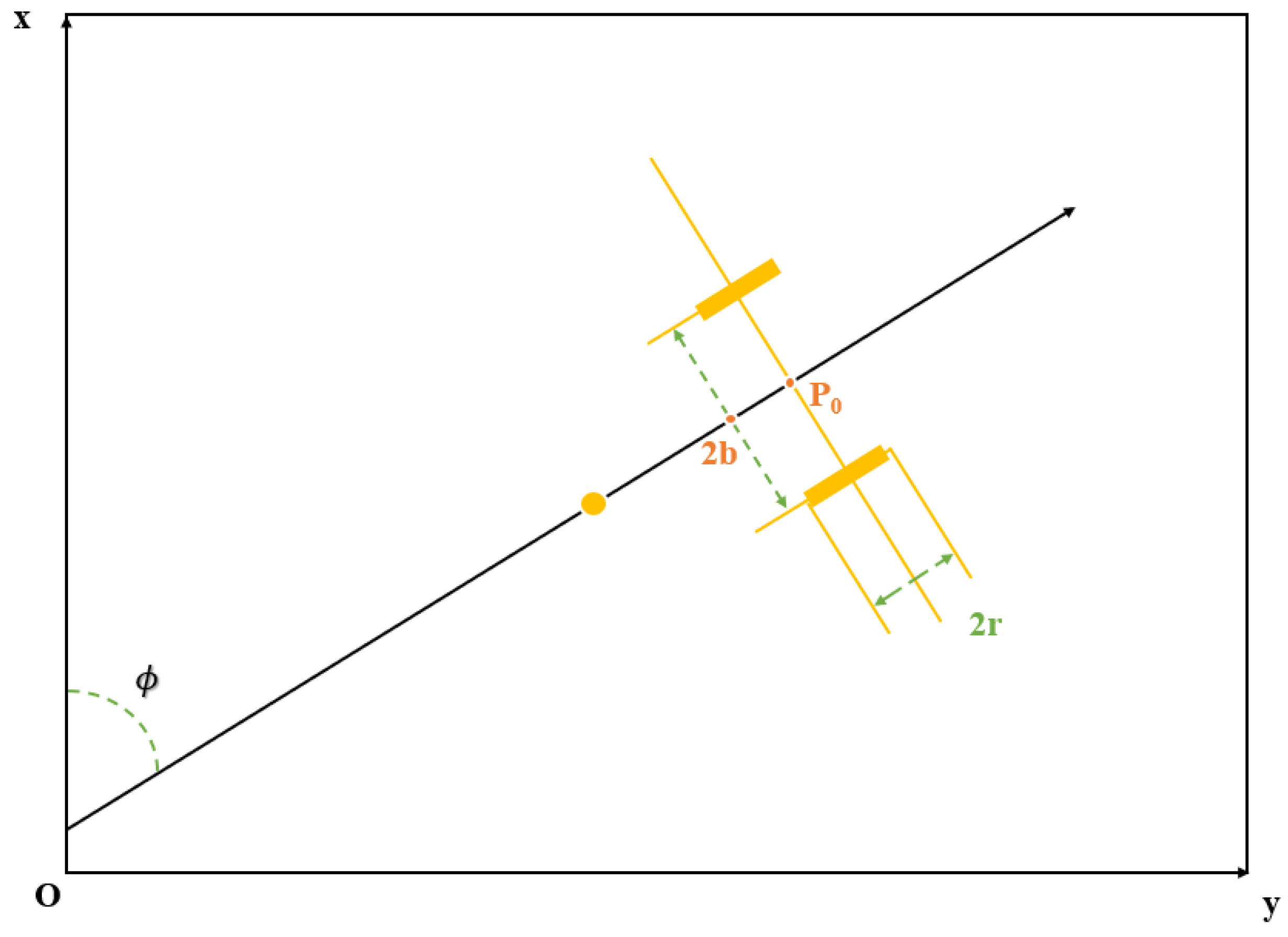
Figure 1 shows a prototype of a two-wheeled mobile robot, which has two driving wheels and one steering wheel. Among them, the two wheels’ drive is itself driven by two motors, and the guide wheel only plays a supporting role. is the world coordinate system and is the mobile robot coordinate system. The bit-case of the mobile robot platform can be represented by the generalized coordinate vector , where represent the position of the robot, represents the heading Angle of the robot, and represent the rotation Angle between the left and right driving wheels, is the distance between the robot wheels, and r is the wheel radius [11].
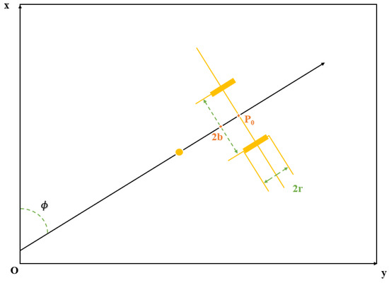
Figure 1.
Wheeled mobile robot model.
Under the condition that the mobile robot satisfies pure rolling and no sliding, the kinematics equation is shown in Formula (1):
It is noteworthy that the condition above leads to non-holonomic constraint equations. The mechanical systems that are subjected to non-holonomic constraints in the general case need equations of motion that are different from Lagrange’s equations of the second kind. Lagrange’s equations with multipliers, Appel’s equations and Chaplygin’s equations are examples of this.
Formula (1) is abbreviated as
Among them, .
Let be a full-rank matrix composed of a series of smooth and linearly independent vectors, which can be obtained by combining the kinematic properties of the mobile robot:
Where . The kinematics equation of the robot is expressed as follows:
where , represents the linear velocity of the mobile robot, and represents the angular velocity of the mobile robot.
In the case of the dynamic equations of a wheel pair, the sum of the additional terms that appear due to non-holonomic constraints is equal to zero. So under this consideration, the equations of motion coincide with Lagrange’s equations of the second kind. The Lagrangian equation with a multiplier of the mobile robot is as follows:
where is a symmetric positive definite inertia matrix, is the central axial force and Coriolis matrix, is the gravity matrix, represents the sum of internal uncertainties and external disturbances of the system, represents the input transformation matrix, represents the input vector, is the matrix related to constraints, and is the Lagrange operator vector.
According to Equation (4) of the robot dynamic model and Equation (3) of kinematics, the final model is obtained as follows:
where represents the input vector
Equation (5) can be written as
The parameter uncertainties, parameter perturbations and input disturbances existing in the mobile robot system are regarded as the sum disturbance of the system, i.e.,
Since the mobile robot works on the horizontal plane, , it can be further obtained as follows:
where
2.3. Description of Trajectory Tracking Problem
Given the reference position and the actual pose of the mobile robot, the error equation of the pose of the mobile robot can be expressed as
Taking the derivative of Equation (8), the following differential equation of trajectory tracking error is obtained:
In order to track the desired trajectory, an auxiliary speed control input is given:
where is the reference linear velocity and steering velocity of the wheeled robot, and are the feedback gain matrices of , respectively.
In order to track the parameter trajectory, the velocity tracking error is introduced as follows:
As the design criterion of the generalized extended observer controller, Equation (11) ensures that the trajectory tracking error of the wheeled robot satisfies by controlling that its velocity tracking error satisfies .
2.4. Design and Analysis of High Precision Interval Observer
A high-precision interval observer is designed to deal with the uncertainties such as system modeling mismatch, internal parameter perturbation and external disturbance in the actual system of the wheeled mobile robot. Real-time estimation and compensation of uncertainties can be realized to improve the robustness of the mobile robot system against disturbances and its adaptability to the environment [12,13,14].
For the dynamic system Equation (5) of the wheeled mobile robot, the following high-precision interval observer is designed:
Define the extension variable , which expands the original system as follows:
where ,
.
Since is observable, for the system shown in Equation (13), the following high precision interval observer design is constructed:
where is the estimated value of the state variable and L is the gain matrix of the observer to be designed.
The control law is designed as
where refers to the senile control gain matrix, and refers to the interference complement gain matrix. The interference is estimated by selecting appropriate and .
2.5. Stability Analysis
Stability is one of the important characteristics of systems, and Lyapunov stability theory is still an effective method to study the stability of systems with linear parameter variations [15].
Define the estimation error system as:
H is called the Hamiltonian energy function, and represent the observed value, z represent the observation error, and ⊤ represent the reversible constant matrix.
Considering the system (16), Order:
The initial condition is satisfied: and , then the system (16) is asymptotically stable and converges to zero.
Proof: The stability of the error system is analyzed below. First, consider , then , where is the error between the assumed approximate compensation function and the real value, and use the method of increasing output filtering and dynamic compensation factor to study:
According to Young’s inequality, there is a variable making the:
The result:
Formula (17) into the Formula (20), then:
Due to , therefore:
The Lyapunov function considering the system (16) is:
Then:
Order:
Then:
Here is the following description: according to Equation (17), it is not difficult to find that . When = 1, in Equation (26), , then , then , so, , and , then converges to zero, tends to zero.
In this paper, the error observation system is transformed into a class of Hamilton system, and the stability and observer design of the system are studied from the overall perspective, which simplifies the proof process.
3. Simulation Results and Discussion
In order to verify the effectiveness of the designed high-precision interval observer control strategy and the tracking performance of the system, the proposed control method is applied to the simulation of a wheeled mobile robot. The parameters of the mobile robot used for the experiment are shown in Table 1 as follows [16,17,18].

Table 1.
Parameters of mobile robot.
According to the robot parameters and variables defined in Table 1, on the premise that the center of mass of the wheeled mobile robot coincides with the geometric center, according to the principle of torque balance, Newton’s second law of motion and the speed regulation principle of the wheeled mobile robot driven by two wheels, the following dynamic model of the wheeled mobile robot is derived:
Among: The and is the variable.
Define the following variables:
Then the kinetic Equations (27) and (28) of the wheeled mobile robot can be expressed as:
In the formula, and represent state, control and output, respectively.
Then we can find that the dynamic equation of the wheeled mobile robot is obtained.
To test the performance of the proposed control method of high-precision interval observer, it is compared with other design methods. This method proposes the following form of interval observer:
and are obtained by solving the equation , and and are obtained by solving the Sylvester equation:
In Equation (33), is the matrix selected by the designer. This method needs to solve the matrix T first, then determine an R matrix and solve (32) to obtain the values of P and Q, and finally obtain the matrix L by [19].
After getting and , we also need to get the interval estimation and of x by the following formula:
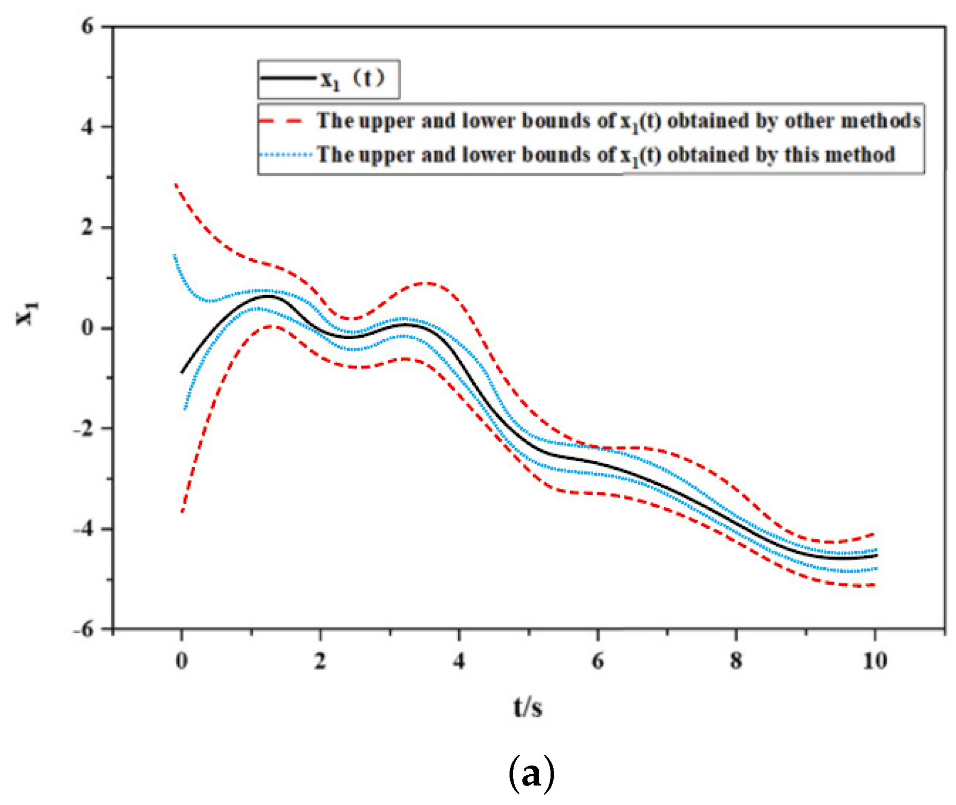
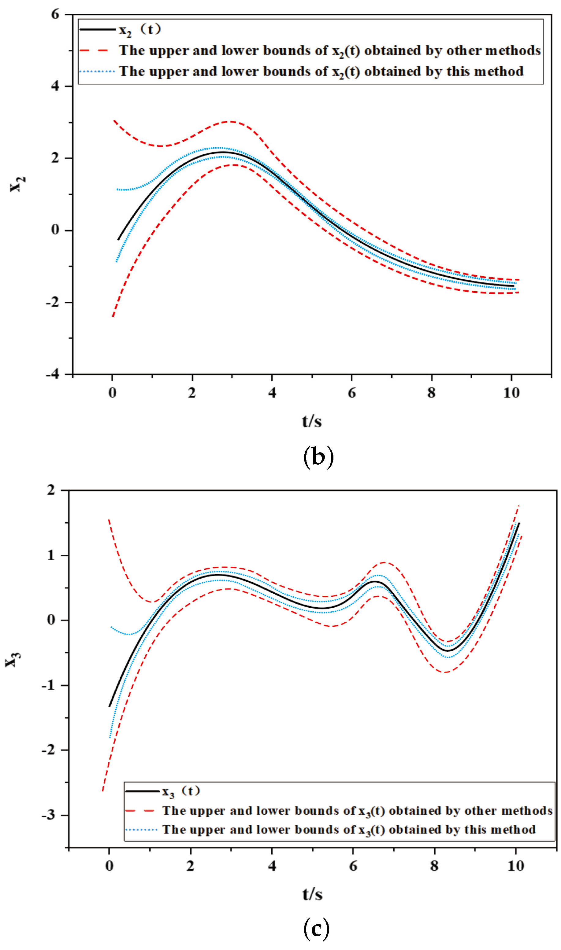
The interval estimation results shown in Figure 2a–c can be obtained by using the method proposed in this paper, where is the state vector, is three state vectors, the blue dotted line shows the upper and lower bounds obtained by the method proposed in this paper, and the red dashed line shows the upper and lower bounds obtained by other methods. The methods used in the results are listed in Table 2.
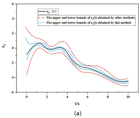
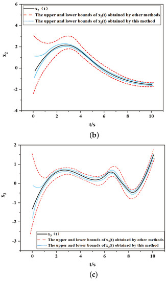
Figure 2.
Results of interval estimation between this method and other methods. (a) and its interval estimation results. (b) and its interval estimation results. (c) and its interval estimation results.
Table 2.
The methods used for the results.
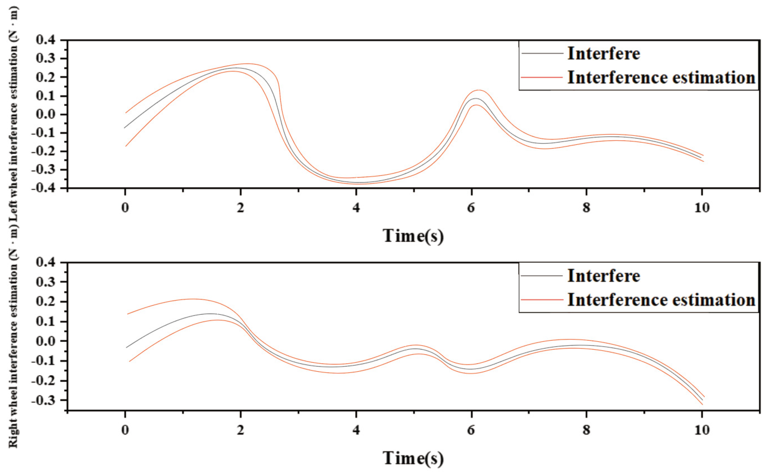
Using the method presented in this paper and the method presented in the literature [20], the interval estimation results are shown in Figure 3. Among them, the red line shows the upper and lower bounds obtained by the proposed method proposed in this paper. It can be seen that the proposed method can obtain a more accurate interval estimation, indicating that the performance of the proposed method is better. This is because the method in the literature [20] is based on coordinate transformation, which designs conditions to some extent, but also brings some conservatism.
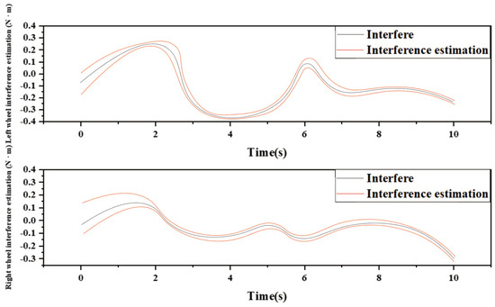
Figure 3.
Velocity tracking and perturbation estimation.
It can be seen that the method proposed in this paper can obtain more accurate interval estimation. This is because other methods are based on coordinate transformation [21,22]. Although the design conditions are relaxed to a certain extent, they also bring a certain degree of conservatism. In fact, if we combine the method in this paper with iterative learning control, the results will be more accurate, which is conducive to our trajectory control of the robot [23,24,25].
4. Conclusions
In this essay, a high-precision interval observer is proposed for the robot system. In this essay, the trajectory tracking problem of high precision interval observer is studied in the case of the uncertainty of control parameters and unknown external disturbance of mobile robots in a complex environment. Firstly, the kinematics and dynamics models of the wheeled mobile robot are derived, and then a controller based on the dynamics model is designed by using a high-precision interval observer. The controller can overcome the influence of unknown disturbances effectively, which not only ensures the stability of the system but also realizes the stability and quick tracking of the trajectory. It should be pointed out that we can also use artificial intelligence or design method can further optimize the performance of the interval observer, which can be considered as one of the future research work [26,27].
Author Contributions
Conceptualization, H.H.; methodology, X.L., Y.C. and H.H.; data curation, S.D. and Z.S.; writing—original draft preparation, S.D.; supervision, X.C. All authors have read and agreed to the published version of the manuscript.
Funding
This work was invested by National Natural Science Foundation of China under Grant 62103293, Natural Science Foundation of Jiangsu Province under Grant BK20210709, Suzhou Municipal Science and Technology Bureau under Grant SYG202138.
Data Availability Statement
Not applicable.
Conflicts of Interest
The authors declare no conflict of interest.
References
- Arents, J.; Greitans, M. Smart industrial robot control trends, challenges and opportunities within manufacturing. Appl. Sci. 2022, 12, 937. [Google Scholar] [CrossRef]
- Lee, C.; An, D. AI-Based Posture Control Algorithm for a 7-DOF Robot Manipulator. Machines 2022, 10, 651. [Google Scholar] [CrossRef]
- Jiang, W.; Chen, Y.; Chen, H.; Schutter, B.D. A Unified Framework for Multi-Agent Formation with a Non-repetitive Leader Trajectory: Adaptive Control and Iterative Learning Control. TechRxiv 2023. [Google Scholar] [CrossRef]
- Jiang, W.; Chen, Y.; Charalambous, T. Consensus of General Linear Multi-Agent Systems with Heterogeneous Input and Communication Delays. IEEE Control. Syst. Lett. 2020, 5, 851–856. [Google Scholar] [CrossRef]
- Ito, H.; Dinh, T.N. Asymptotic and tracking guarantees in interval observer design for systems with unmeasured polytopic nonlinearities. IFAC-PapersOnLine 2020, 53, 5010–5015. [Google Scholar] [CrossRef]
- Garbouj, Y.; Dinh, T.N.; Raissi, T.; Zouari, T.; Ksouri, M. Optimal interval observer for switched takagi–sugeno systems: An application to interval fault estimation. IEEE Trans. Fuzzy Syst. Publ. IEEE Neural Netw. Counc. 2020, 29, 2296–2309. [Google Scholar] [CrossRef]
- Khajenejad, M.; Jin, Z.; Yong, S.Z. Resilient interval observer for simultaneous estimation of states, modes and attack policies. In Proceedings of the 2022 American Control Conference (ACC), Atlanta, GA, USA, 8–10 June 2022. [Google Scholar]
- Harlamov, B.P.; Rasova, S.S. Time distribution from zero up to beginning: Of the final stop of semi-markov diffusion process on interval with unattainable boundaries. Vestnik St. Petersburg University. Mathematics 2022, 9, 38309. [Google Scholar]
- D’Angelo, G.; Perrett, A.; Iacono, M.; Furber, S.; Bartolozzi, C. Event Driven Bio-Inspired Attentive System for the Icub Humanoid Robot on Spinnaker; IOP Publishing Ltd.: Bristol, UK, 2022. [Google Scholar]
- Bingul, Z.; Karahan, O. Real-time trajectory tracking control of stewart platform using fractional order fuzzy pid controller optimized by particle swarm algorithm. Ind. Robot. 2022, 49, 708–725. [Google Scholar] [CrossRef]
- Neimark, J.I.; Fufaev, N.A. Dynamics of Nonholonomic Systems; Translations of Mathematical Monographs; American Mathematical Society: Providence, RI, USA, 1972; Volume 33. [Google Scholar]
- Dmmer, G.; Bauer, H.; Rüdiger, N.; Major, Z. Design, additive manufacturing and component testing of pneumatic rotary vane actuators for lightweight robots. Rapid Prototyp. J. 2022, 28, 20–32. [Google Scholar] [CrossRef]
- Zhang, S.; Shan, J.; Sun, F.; Fang, B.; Yang, Y. Multimode fusion perception for transparent glass recognition. Ind. Robot. Int. J. Robot. Res. Appl. 2022, 49, 625–633. [Google Scholar] [CrossRef]
- Liu, Q.; Cai, Z.; Chen, J.; Jiang, B. Observer-based integral sliding mode control of nonlinear systems with application to single-link flexible joint robotics. Complex Eng. Syst. 2021, 1, 8. [Google Scholar] [CrossRef]
- Briskin, E.S.; Kalinin, Y.V.; Smirnaya, L.D. On determining the optimal lifting law of the walking propulsion device foot of an underwater robot from the bottom. J. Artif. Intell. Technol. 2021, 1, 214–218. [Google Scholar] [CrossRef]
- Liang, C.; Zhang, Z.; Wu, Q.; Li, X. Barrier lyapunov function-based robot control with an augmented neural network approximator. Ind. Robot. 2022, 49, 359–367. [Google Scholar]
- Martínez-Rozas, S.; Alejo, D.; Caballero, F.; Merino, L. Path and trajectory planning of a tethered uav-ugv marsupial robotics system. arXiv 2022, arXiv:2204.01828. [Google Scholar]
- Mitra, R.; Jaramaz, B. Navio Surgical System—Handheld Robotics-Science Direct. Handbook of Robotic and Image-Guided Surgery; Elsevier: Amsterdam, The Netherlands, 2020; pp. 443–457. [Google Scholar] [CrossRef]
- Harib, M.; Chaoui, H.; Miah, S. Evolution of adaptive learning for nonlinear dynamic systems: A systematic survey. Intell. Robot. 2022, 2, 37–71. [Google Scholar] [CrossRef]
- Guo, S.H.; Zhu, F. Interval observers design for descriptor systems. Control. Decis. 2016, 31, 361–366. [Google Scholar]
- Khajenejad, M.; Shoaib, F.; Yong, S.Z. Interval observer synthesis for locally lipschitz nonlinear dynamical systems via mixed-monotone decompositions. In Proceedings of the 2022 American Control Conference (ACC), Atlanta, GA, USA, 8–10 June 2022. [Google Scholar]
- Song, X.; Lam, J.; Zhu, B.; Fan, C. Interval observer-based fault-tolerant control for a class of positive markov jump systems. Inf. Sci. Int. J. 2022, 590, 142–157. [Google Scholar] [CrossRef]
- Zhuang, Z.; Tao, H.; Chen, Y.; Stojanovicc, V.; Paszke, W. An Optimal Iterative Learning Control Approach for Linear Systems with Nonuniform Trial Lengths under Input Constraints. IEEE Trans. Syst. Man, Cybern. Syst. 2022. [Google Scholar] [CrossRef]
- Chen, Y.; Chu, B.; Freeman, C.T. Iterative Learning Control for Robotic Path Following With Trial-Varying Motion Profiles. IEEE/ASME Trans. Mechatronics 2022, 27, 4697–4706. [Google Scholar] [CrossRef]
- Chen, Y.; Jiang, W.; Charalambous, T. Machine learning based iterative learning control for non-repetitive time-varying systems. Int. J. Robust Nonlinear Control. 2022. [Google Scholar] [CrossRef]
- Ge, P.; Chen, Y.; Wang, G.; Weng, G. An active contour model driven by adaptive local pre-fitting energy function based on Jeffreys divergence for image segmentation. Expert Syst. Appl. 2022, 210, 118493. [Google Scholar] [CrossRef]
- Wang, G.; Zhang, F.; Chen, Y.; Weng, G.; Chen, H. An Active Contour Model Based on Local Pre-piecewise Fitting Bias Corrections for Fast and Accurate Segmentation. IEEE Trans. Instrum. Meas. 2023, 72, 5006413. [Google Scholar] [CrossRef]
Disclaimer/Publisher’s Note: The statements, opinions and data contained in all publications are solely those of the individual author(s) and contributor(s) and not of MDPI and/or the editor(s). MDPI and/or the editor(s) disclaim responsibility for any injury to people or property resulting from any ideas, methods, instructions or products referred to in the content. |
© 2023 by the authors. Licensee MDPI, Basel, Switzerland. This article is an open access article distributed under the terms and conditions of the Creative Commons Attribution (CC BY) license (https://creativecommons.org/licenses/by/4.0/).