
Robotic Arm Position Computing Method in the 2D and 3D Spaces


Abstract
1. Introduction
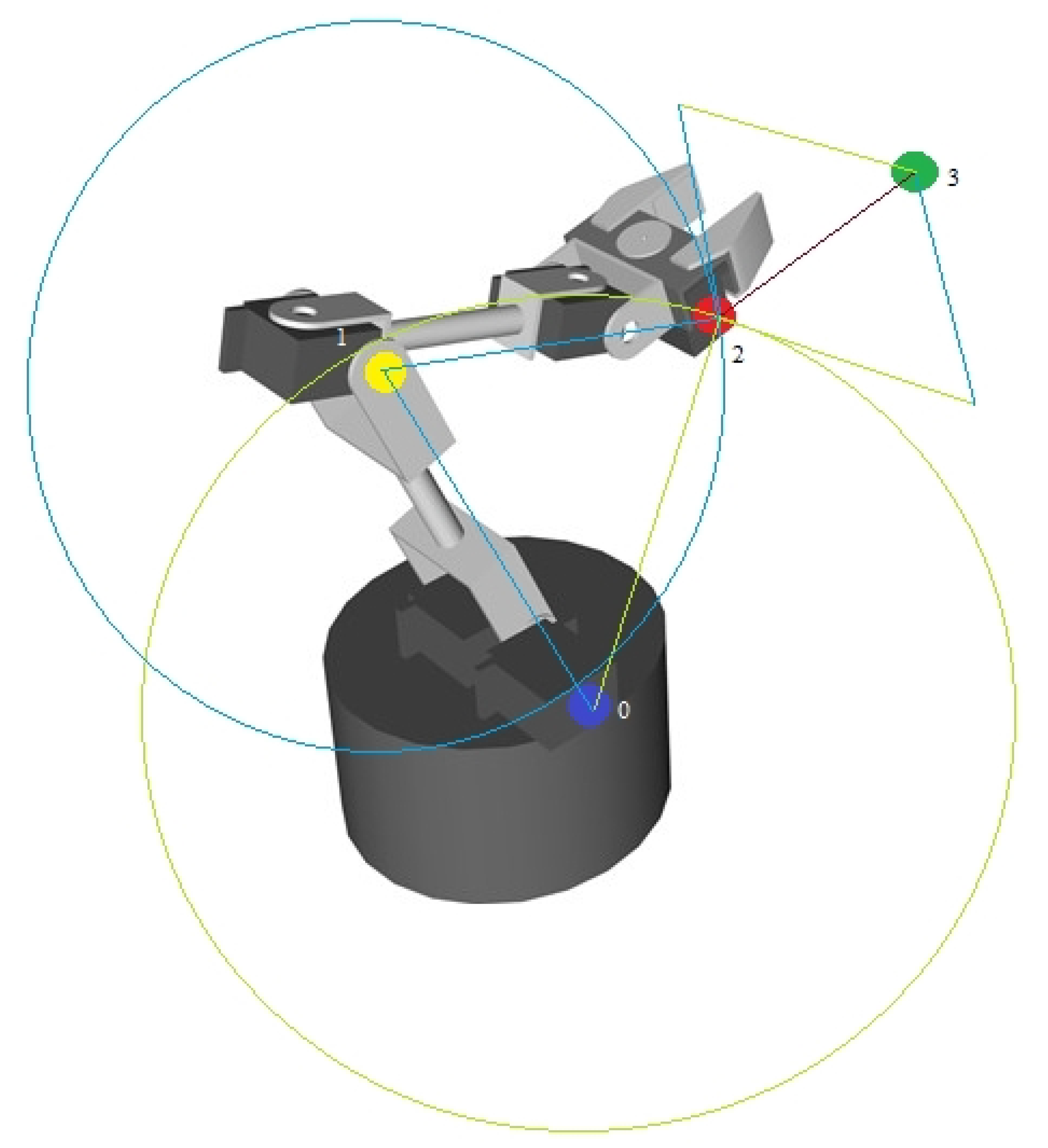
2. Problem Solving
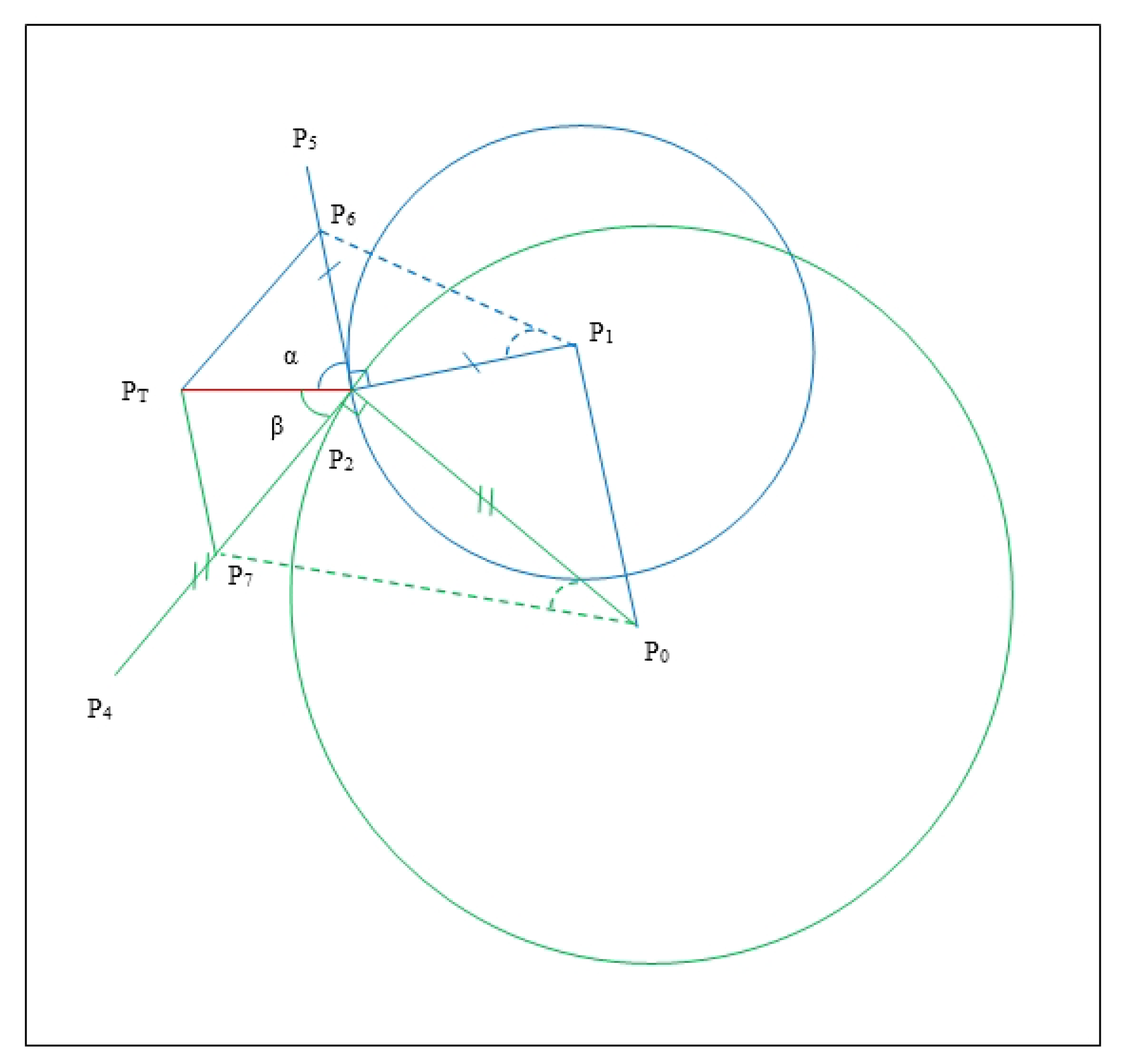
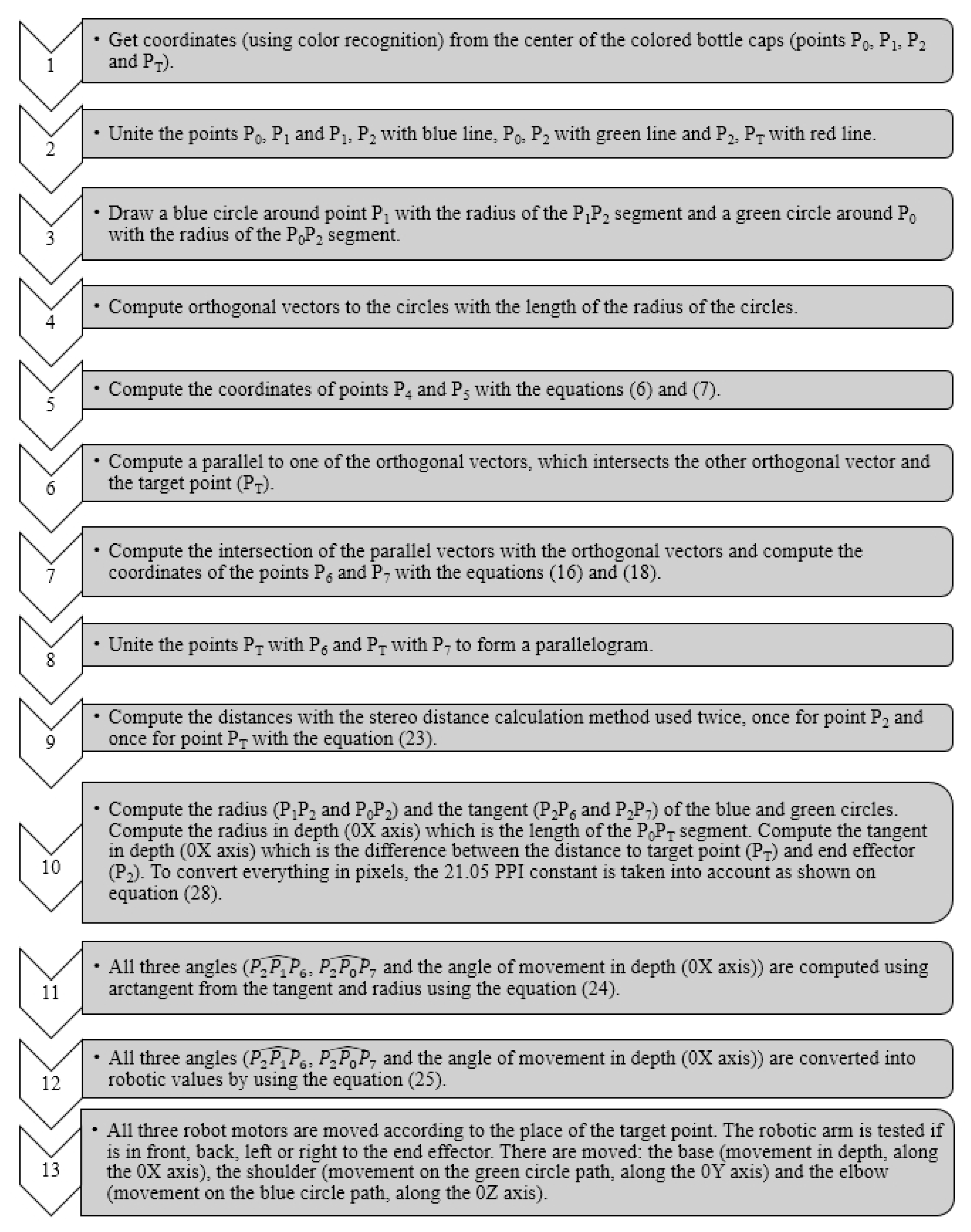
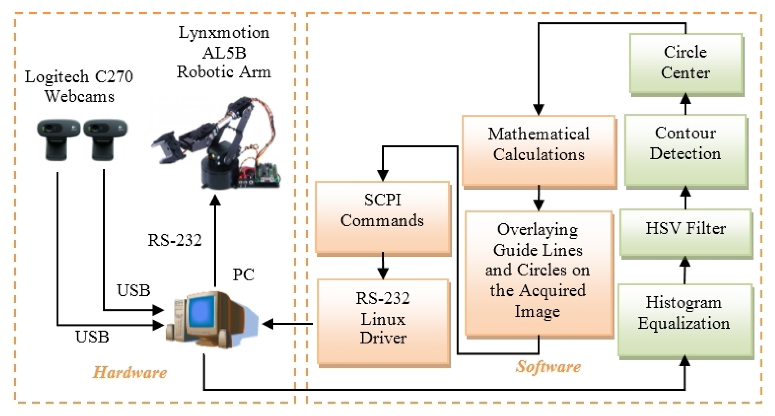
2.1. Presenting the Proposed Algorithm
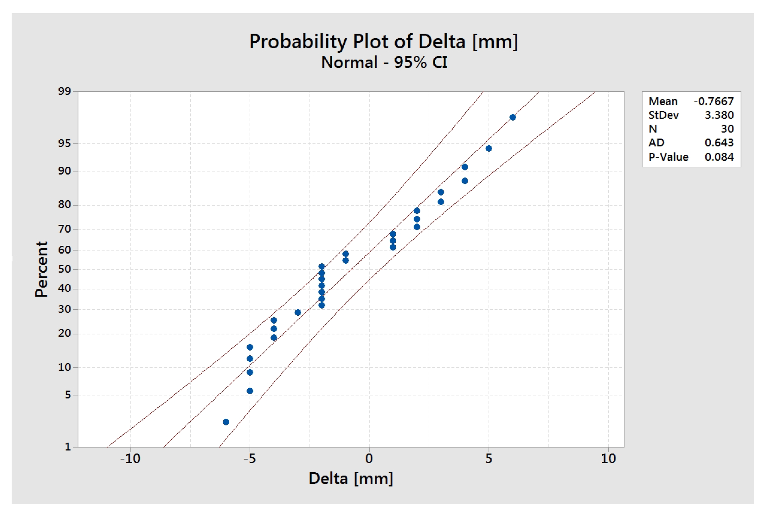
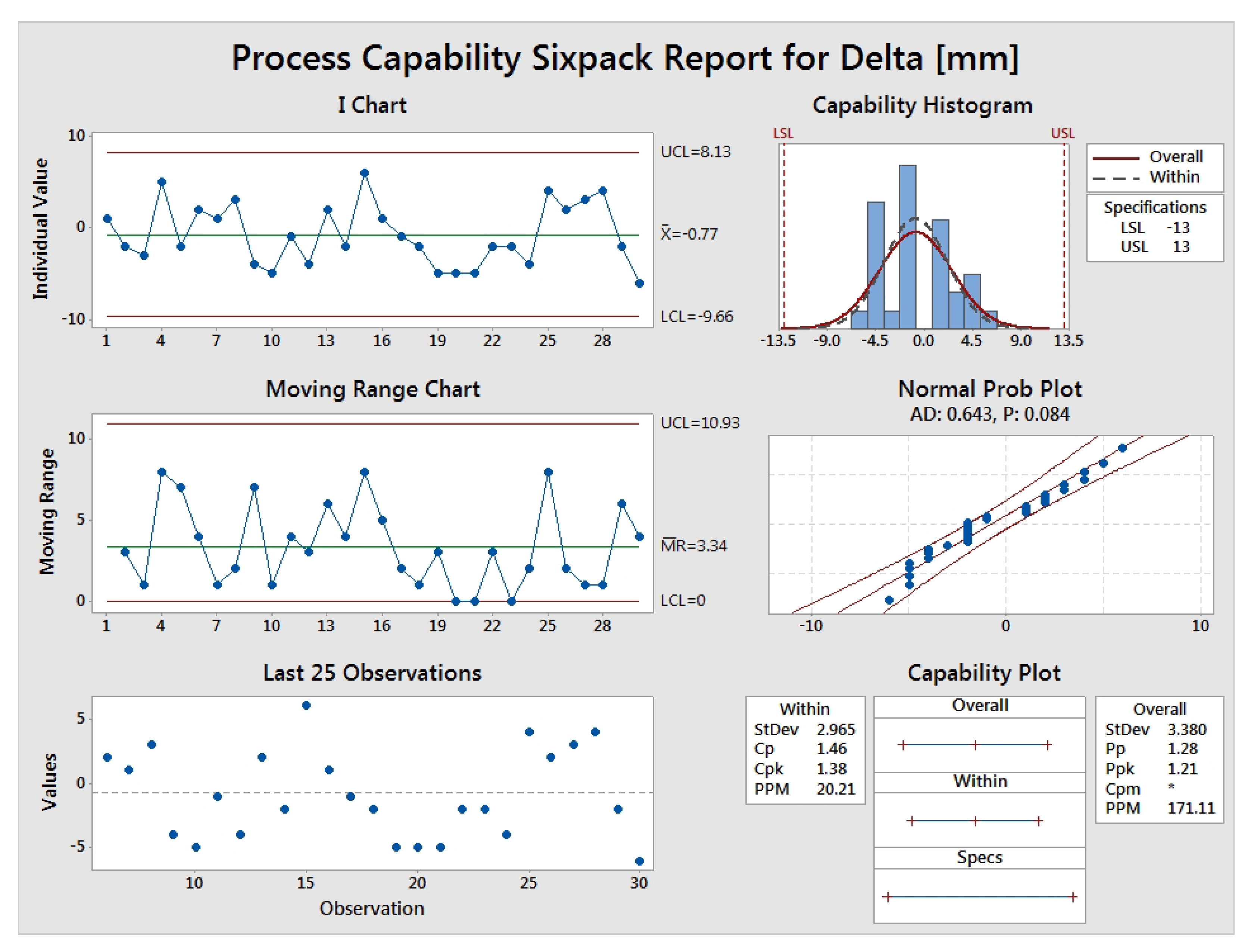
2.2. Method Evaluation with Six-Sigma Tools
3. Results
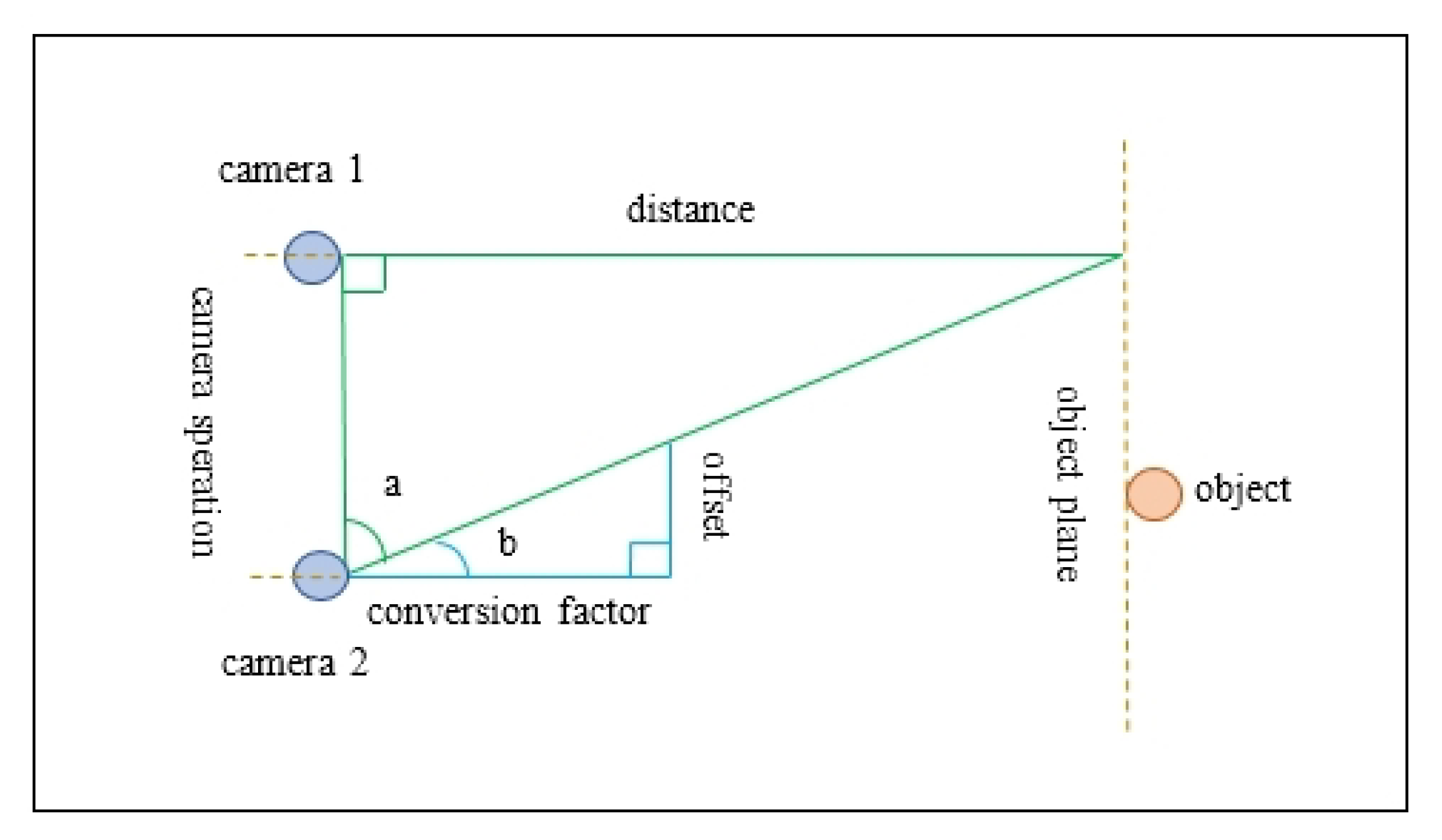
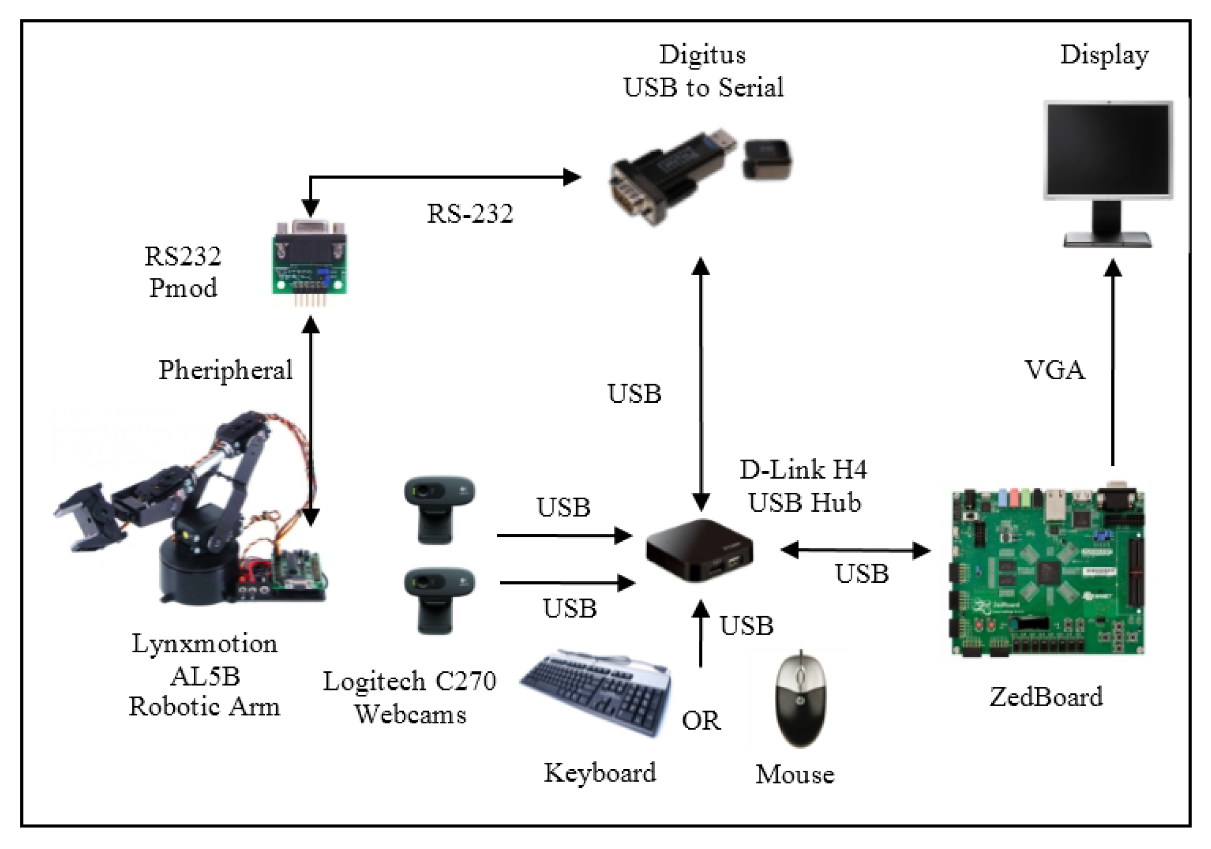
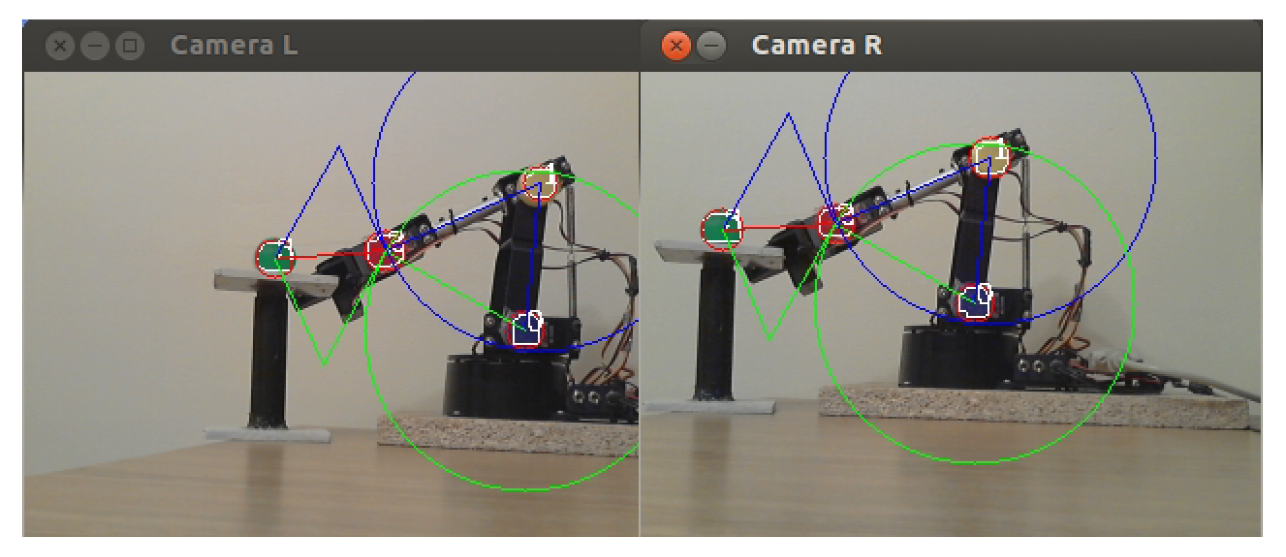
3.1. Calibrations
3.2. Experimental Results
3.3. Discussion
4. Conclusions
Author Contributions
Funding
Data Availability Statement
Acknowledgments
Conflicts of Interest
Notations
| 2D | 2 Dimensions |
| 3D | 3 Dimensions |
| DoF | Degrees of Freedom |
| difference between robotic values (pulse widths) of the motors of the robotic arm | |
| difference between vectors | |
| vectors | |
| length of the Euclidean norm vector | |
| orthogonal vectors | |
| slopes of the two tangents to the circles | |
| right and left points of the offset | |
| pi = 3.14 | |
| inch | |
| Pixels Per Inch | |
| right, left | |
| coordinates | |
| d | distance |
| f | focal distance |
| angle | |
| coordinates in space | |
| vectors of the coordinates in space | |
| unit vectors | |
| vectors | |
| scalars | |
| vectors | |
| USB | Universal Serial Bus |
| RS-232 | Recommended Standard 232 (serial communication) |
| PC | Personal Computer |
| HSV | Hue, Saturation, Value |
| SCPI | Standard Commands for Programmable Instruments |
| ARM | Advanced RISC (Reduced Instruction Set Computer) Machine |
| SoC | System-on-a-Chip |
| FPGA | Field Programmable Gate Array |
| OpenCV | Open Computer Vision |
| UART | Universal Asynchronous Receiver-Transmitter (serial communication) |
| VGA | Video Graphics Array |
| HDMI | High-Definition Multimedia Interface |
| GPU | Graphics Processing Unit |
Appendix A


References
- Lippiello, V.; Ruggiero, F.; Siciliano, B.; Villani, L. Visual Grasp Planning for Unknown Objects Using a Multifingered Robotic Hand. IEEE/ASME Trans. Mechatron. 2013, 18, 1050–1059. [Google Scholar] [CrossRef]
- Kazemi, M.; Gupta, K.K.; Mehrandezh, M. Randomized Kinodynamic Planning for Robust Visual Servoing. IEEE Trans. Robot. 2013, 29, 1197–1211. [Google Scholar] [CrossRef]
- Fomena, R.T.; Tahri, O.; Chaumette, F. Distance-Based and Orientation-Based Visual Servoing from Three Points. IEEE Trans. Robot. 2011, 27, 256–267. [Google Scholar] [CrossRef]
- Heuring, J.J.; Murray, D.W. Modeling and copying human head movements. IEEE Trans. Robot. Autom. 1999, 15, 1095–1108. [Google Scholar] [CrossRef]
- Chaumette, F.; Hutchinson, S. Visual servo control. II. Advanced approaches [Tutorial]. IEEE Robot. Autom. Mag. 2007, 14, 109–118. [Google Scholar] [CrossRef]
- Naceri, A.; Schumacher, T.; Li, Q.; Calinon, S.; Ritter, H. Learning Optimal Impedance Control during Complex 3D Arm Movements. IEEE Robot. Autom. Lett. 2021, 6, 1248–1255. [Google Scholar] [CrossRef]
- Li, S.; Zhang, Y.; Jin, L. Kinematic Control of Redundant Manipulators Using Neural Networks. IEEE Trans. Neural Netw. Learn. Syst. 2017, 28, 2243–2254. [Google Scholar] [CrossRef]
- Jiang, Y.; Wang, Y.; Miao, Z.; Na, J.; Zhao, Z.; Yang, C. Composite-Learning-Based Adaptive Neural Control for Dual-Arm Robots With Relative Motion. IEEE Trans. Neural Netw. Learn. Syst. 2022, 33, 1010–1021. [Google Scholar] [CrossRef]
- Vazquez, L.A.; Jurado, F.; Castaneda, C.E.; Santibanez, V. Real-Time Decentralized Neural Control via Backstepping for a Robotic Arm Powered by Industrial Servomotors. IEEE Trans. Neural Netw. Learn. Syst. 2018, 29, 419–426. [Google Scholar] [CrossRef]
- Liu, Z.; Chen, C.; Zhang, Y.; Chen, C.L.P. Adaptive Neural Control for Dual-Arm Coordination of Humanoid Robot With Unknown Nonlinearities in Output Mechanism. IEEE Trans. Cybern. 2015, 45, 507–518. [Google Scholar]
- Cheng, B.; Wu, W.; Tao, D.; Mei, S.; Mao, T.; Cheng, J. Random Cropping Ensemble Neural Network for Image Classification in a Robotic Arm Grasping System. IEEE Trans. Instrum. Meas. 2020, 69, 6795–6806. [Google Scholar] [CrossRef]
- Freire, E.O.; Rossomando, F.G.; Soria, C.M. Self-tuning of a Neuro-Adaptive PID Controller for a SCARA Robot Based on Neural Network. IEEE Lat. Am. Trans. 2018, 16, 1364–1374. [Google Scholar] [CrossRef]
- Zhang, Y.; Chen, S.; Li, S.; Zhang, Z. Adaptive Projection Neural Network for Kinematic Control of Redundant Manipulators with Unknown Physical Parameters. IEEE Trans. Ind. Electron. 2018, 65, 4909–4920. [Google Scholar] [CrossRef]
- Hu, Z.; Han, T.; Sun, P.; Pan, J.; Manocha, D. 3D Deformable Object Manipulation Using Deep Neural Networks. IEEE Robot. Autom. Lett. 2019, 4, 4255–4261. [Google Scholar] [CrossRef]
- Huang, X.; Wu, W.; Qiao, H.; Ji, Y. 3D Brain-Inspired Motion Learning in Recurrent Neural Network with Emotion Modulation. IEEE Trans. Cogn. Dev. Syst. 2018, 10, 1153–1164. [Google Scholar] [CrossRef]
- Yang, Y.; Ni, Z.; Gao, M.; Zhang, J.; Tao, D. Collaborative Pushing and Grasping of Tightly Stacked Objects via Deep Reinforcement Learning. IEEE/CAA J. Autom. Sin. 2022, 9, 135–145. [Google Scholar] [CrossRef]
- Zhang, T.; Zhang, K.; Lin, J.; Louie, W.-Y.G.; Huang, H. Sim2real Learning of Obstacle Avoidance for Robotic Manipulators in Uncertain Environments. IEEE Robot. Autom. Lett. 2022, 7, 65–72. [Google Scholar] [CrossRef]
- Hsieh, Y.-Z.; Lin, S.-S. Robotic Arm Assistance System Based on Simple Stereo Matching and Q-Learning Optimization. IEEE Sens. J. 2020, 20, 10945–10954. [Google Scholar] [CrossRef]
- James, S.; Davison, A.J. Q-Attention: Enabling Efficient Learning for Vision-Based Robotic Manipulation. IEEE Robot. Autom. Lett. 2022, 7, 1612–1619. [Google Scholar] [CrossRef]
- Yang, D.; Liu, H.A. EMG-Based Deep Learning Approach for Multi-DOF Wrist Movement Decoding. IEEE Trans. Ind. Electron. 2022, 69, 7099–7108. [Google Scholar] [CrossRef]
- Seelinger, M.; Gonzalez-Galvan, E.; Robinson, M.; Skaar, S. Towards a robotic plasma spraying operation using vision. IEEE Robot. Autom. Mag. 1998, 5, 33–38. [Google Scholar] [CrossRef]
- Kelly, R.; Carelli, R.; Nasisi, O.; Kuchen, B.; Reyes, F. Stable visual servoing of camera-in-hand robotic systems. IEEE/ASME Trans. Mechatron. 2000, 5, 39–48. [Google Scholar] [CrossRef]
- Behera, L.; Kirubanandan, N. A hybrid neural control scheme for visual-motor coordination. IEEE Control Syst. 1999, 19, 34–41. [Google Scholar]
- Park, I.-W.; Lee, B.-J.; Cho, S.-H.; Hong, Y.-D.; Kim, J.-H. Laser-Based Kinematic Calibration of Robot Manipulator Using Differential Kinematics. IEEE/ASME Trans. Mechatron. 2012, 17, 1059–1067. [Google Scholar] [CrossRef]
- Li, Z.; Li, S.; Luo, X. Using Quadratic Interpolated Beetle Antennae Search to Enhance Robot Arm Calibration Accuracy. IEEE Robot. Autom. Lett. 2022, 7, 107202–107213. [Google Scholar] [CrossRef]
- Tan, N.; Yu, P.; Zhong, Z.; Ni, F. A New Noise-Tolerant Dual-Neural-Network Scheme for Robust Kinematic Control of Robotic Arms with Unknown Models. IEEE/CAA J. Autom. Sin. 2022, 9, 1778–1791. [Google Scholar] [CrossRef]
- Costanzo, M.; De Maria, G.; Natale, C. Tactile Feedback Enabling In-Hand Pivoting and Internal Force Control for Dual-Arm Cooperative Object Carrying. IEEE Robot. Autom. Lett. 2022, 7, 11466–11473. [Google Scholar] [CrossRef]
- AlBeladi, A.; Ripperger, E.; Hutchinson, S.; Krishnan, G. Hybrid Eye-in-Hand/Eye-to-Hand Image Based Visual Servoing for Soft Continuum Arms. IEEE Robot. Autom. Lett. 2022, 7, 11298–11305. [Google Scholar] [CrossRef]
- Ruan, Q.; Yang, F.; Yue, H.; Li, Q.; Xu, J.; Liu, R. An Accurate Position Acquisition Method of a Hyper-Redundant Arm with Load. IEEE Sens. J. 2022, 22, 8986–8995. [Google Scholar] [CrossRef]
- Rakshit, A.; Konar, A.; Nagar, A.K. A hybrid brain-computer interface for closed-loop position control of a robot arm. IEEE/CAA J. Autom. Sin. 2020, 7, 1344–1360. [Google Scholar] [CrossRef]
- Li, F.; Jiang, Y.; Li, T. A Laser-Guided Solution to Manipulate Mobile Robot Arm Terminals within a Large Workspace. IEEE/ASME Trans. Mechatron. 2021, 26, 2676–2687. [Google Scholar] [CrossRef]
- Tang, Z.; Wang, P.; Xin, W.; Laschi, C. Learning-Based Approach for a Soft Assistive Robotic Arm to Achieve Simultaneous Position and Force Control. IEEE Robot. Autom. Lett. 2022, 7, 8315–8322. [Google Scholar] [CrossRef]
- Min, J.-K.; Kim, D.-W.; Song, J.-B. A Wall-Mounted Robot Arm Equipped with a 4-DOF Yaw-Pitch-Yaw-Pitch Counterbalance Mechanism. IEEE Robot. Autom. Lett. 2020, 5, 3768–3774. [Google Scholar] [CrossRef]
- Lu, W.; Tang, B.; Wu, Y.; Lu, K.; Wang, D.; Wang, X. A New Position Detection and Status Monitoring System for Joint of SCARA. IEEE/ASME Trans. Mechatron. 2021, 26, 1613–1623. [Google Scholar] [CrossRef]
- Khaled, T.A.; Akhrif, O.; Bonev, I.A. Dynamic Path Correction of an Industrial Robot Using a Distance Sensor and an ADRC Controller. IEEE/ASME Trans. Mechatron. 2021, 26, 1646–1656. [Google Scholar] [CrossRef]
- Kamtikar, S.; Marri, S.; Walt, B.; Uppalapati, N.K.; Krishnan, G.; Chowdhary, G. Visual Servoing for Pose Control of Soft Continuum Arm in a Structured Environment. IEEE Robot. Autom. Lett. 2022, 7, 5504–5511. [Google Scholar] [CrossRef]
- Liu, X.; Madhusudanan, H.; Chen, W.; Li, D.; Ge, J.; Ru, C.; Sun, Y. Fast Eye-in-Hand 3D Scanner-Robot Calibration for Low Stitching Errors. IEEE Trans. Ind. Electron. 2021, 68, 8422–8432. [Google Scholar] [CrossRef]
- Szabo, R.; Gontean, A. Controlling a Robotic Arm in the 3D Space with Stereo Vision. In Proceedings of the 21st Telecommunications Forum (TELFOR), Belgrade, Serbia, 26 November 2013; pp. 916–919. [Google Scholar]
- Santoni, F.; De Angelis, A.; Skog, I.; Moschitta, A.; Carbone, P. Calibration and Characterization of a Magnetic Positioning System Using a Robotic Arm. IEEE Trans. Instrum. Meas. 2019, 68, 1494–1502. [Google Scholar] [CrossRef]
- Zhang, J.; Wang, W.; Cai, Y.; Li, J.; Zeng, Y.; Chen, L.; Yuan, F.; Ji, Z.; Wang, Y.; Wyrwa, J. A Novel Single-Arm Stapling Robot for Oral and Maxillofacial Surgery—Design and Verification. IEEE Robot. Autom. Lett. 2022, 7, 1348–1355. [Google Scholar] [CrossRef]
- Ozguner, O.; Shkurti, T.; Huang, S.; Hao, R.; Jackson, R.C.; Newman, W.S.; Cavusoglu, M. Cenk Camera-Robot Calibration for the Da Vinci Robotic Surgery System. IEEE Trans. Autom. Sci. Eng. 2020, 17, 2154–2161. [Google Scholar] [CrossRef]
- Pan, Y.; Wang, H.; Li, X.; Yu, H. Adaptive Command-Filtered Backstepping Control of Robot Arms with Compliant Actuators. IEEE Trans. Control Syst. Technol. 2018, 26, 1149–1156. [Google Scholar] [CrossRef]
- PPI Computation. Available online: https://www.sven.de/dpi (accessed on 15 September 2022).
- Szabo, R.; Gontean, A. Lynxmotion AL5 Type Robotic Arm Control with Color Detection on FPGA Running Linux OS. In Proceedings of the 24th Telecommunications Forum (TELFOR), Belgrade, Serbia, 22–23 November 2016; pp. 818–821. [Google Scholar]


| Characteristics | Proposed Approach | M. Seelinger [21] | R. Kelly [22] | V. Lippiello [1] | M. Kazemi [2] |
| Joint number | 3 | 6 | 2 | multi-finger | 6 |
| Cost | low | low | low | high | low |
| Precision | high | high | high | high | high |
| Complexity | low | medium | low | high | high |
| Memory Usage | low | medium | low | high | high |
| Calibration Needed | no | yes | yes | yes | yes |
| Characteristics | R.T. Fomena [3] | L. Behera [23] | J.J. Heuring [4] | F. Chaumette [5] | In-Won Park [24] |
| Joint number | 6 | 3 | 6 | 6 | 7 or 4 |
| Cost | low | low | low | low | low |
| Precision | high | high | high | high | high |
| Complexity | high | low | high | high | medium |
| Memory Usage | high | low | high | high | medium |
| Calibration Needed | yes | yes | yes | yes | yes |
| Real Distance (RD) [mm] | Computed Distance (CD) [mm] | Delta () [mm] | Relative Error (RE) |
|---|---|---|---|
| 100 | 99 | 1 | 0.01 |
| 200 | 202 | −2 | 0.01 |
| 300 | 303 | −3 | 0.01 |
| 400 | 395 | 5 | 0.013 |
| 500 | 502 | −2 | 0.004 |
| 600 | 598 | 2 | 0.003 |
| 700 | 699 | 1 | 0.001 |
| 800 | 797 | 3 | 0.004 |
| 900 | 904 | −4 | 0.004 |
| 1000 | 1005 | −5 | 0.005 |
| 1100 | 1101 | −1 | 0.001 |
| 1200 | 1204 | −4 | 0.003 |
| 1300 | 1298 | 2 | 0.002 |
| 1400 | 1402 | −2 | 0.001 |
| 1500 | 1494 | 6 | 0.004 |
| 1600 | 1599 | 1 | 0.001 |
| 1700 | 1701 | −1 | 0.001 |
| 1800 | 1802 | −2 | 0.001 |
| 1900 | 1905 | −5 | 0.003 |
| 2000 | 2005 | −5 | 0.003 |
| 2100 | 2105 | −5 | 0.002 |
| 2200 | 2202 | −2 | 0.001 |
| 2300 | 2302 | −2 | 0.001 |
| 2400 | 2404 | −4 | 0.002 |
| 2500 | 2496 | 4 | 0.002 |
| 2600 | 2598 | 2 | 0.001 |
| 2700 | 2697 | 3 | 0.001 |
| 2800 | 2796 | 4 | 0.001 |
| 2900 | 2902 | −2 | 0.001 |
| 3000 | 3006 | −6 | 0.002 |
Disclaimer/Publisher’s Note: The statements, opinions and data contained in all publications are solely those of the individual author(s) and contributor(s) and not of MDPI and/or the editor(s). MDPI and/or the editor(s) disclaim responsibility for any injury to people or property resulting from any ideas, methods, instructions or products referred to in the content. |
© 2023 by the authors. Licensee MDPI, Basel, Switzerland. This article is an open access article distributed under the terms and conditions of the Creative Commons Attribution (CC BY) license (https://creativecommons.org/licenses/by/4.0/).
Share and Cite
Szabo, R.; Ricman, R.-S. Robotic Arm Position Computing Method in the 2D and 3D Spaces. Actuators 2023, 12, 112. https://doi.org/10.3390/act12030112
Szabo R, Ricman R-S. Robotic Arm Position Computing Method in the 2D and 3D Spaces. Actuators. 2023; 12(3):112. https://doi.org/10.3390/act12030112
Chicago/Turabian StyleSzabo, Roland, and Radu-Stefan Ricman. 2023. "Robotic Arm Position Computing Method in the 2D and 3D Spaces" Actuators 12, no. 3: 112. https://doi.org/10.3390/act12030112
APA StyleSzabo, R., & Ricman, R.-S. (2023). Robotic Arm Position Computing Method in the 2D and 3D Spaces. Actuators, 12(3), 112. https://doi.org/10.3390/act12030112