Abstract
In this study, a novel field-oriented control (FOC) algorithm was proposed in a 60° coordinate system for controlling the speed of permanent magnet synchronous motors. The FOC algorithm consists of several parts in which the reference currents and feedback currents are transformed into the representation form in a 60° coordinate system. Current regulators are typically used in a 60° coordinate system to directly obtain the reference voltage vector. The proposed FOC structure was established by incorporating the space vector pulse width modulation algorithm in a 60° coordinate system. The proposed FOC structure simplified the FOC algorithm and reduced its computational burden. The feasibility of the proposed method was verified through simulations and experiments.
1. Introduction
Permanent magnet synchronous motors (PMSMs) are excited by permanent magnets. PMSMs are widely used in numerous applications because they exhibit a simple, small, and lightweight structure with high reliability and high power density [1,2,3]. Two popular methods, namely field-oriented control (FOC) and direct torque control (DTC), are typically used to control the speed of PMSMs [4]. The FOC mechanism is used to perform current trajectory tracking. In the orthogonal rotating coordinate system (dq frame), the current control objects are DC components, which are used to realize the decoupling of the excitation component and the torque component of the current [5,6]. The objective of the DTC is flux trajectory tracking, which can be used to realize the constant amplitude of the stator flux and fast response of electromagnetic torque [7,8]. The control schemes operate with closed torque and flux loops without current controllers in the DTC while the FOC schemes always contain current loops [9,10].
In the conventional FOC algorithm for two-level three-phase PMSM, the d-axis and q-axis of voltage vectors were obtained by the controllers of the current components in the dq frame. Subsequently, the vectors were transformed into the voltage vector components in the two-phase orthogonal static coordinate system (αβ frame) [11,12]. To improve DC-link voltage utilization, the space vector pulse width modulation (SVPWM) algorithm is typically used to synthesize the reference voltage vector [13,14,15]. The conventional SVPWM algorithm is implemented in an αβ frame. The determination of the sector in which the reference voltage vector is located and the calculation of the action time of the basic voltage vector require numerous complex calculations, which are time-consuming [16,17,18]. Scholars have studied the method of simplifying inverter modulation, especially for multilevel inverters. [19] presented a fast new SVM algorithm for multilevel three-phase converters. [20] presented a new space vector pulse width modulation (SVPWM) scheme for multilevel inverters, which generates all the available switching states and switching sequences based on two simple general mappings and calculates the duty cycles of the nearest three vectors simply as for a two-level SVPWM. [21] presents a new modulation approach for the complete control of the neutral-point voltage in the three-level three-phase neutral-point-clamped voltage source inverter. [22] explored the mathematical model and control method of the neutral-point voltage balancing problem in a three-level NPC inverter. [23] proposes a neutral-point ac ripple voltage reduction method to mitigate the ac unbalance of the neutral-point voltage when the CB-PWM method is applied. If the SVPWM algorithm is implemented in the 60° coordinate system, the code execution time can be reduced considerably, which improves the real-time performance of the system. [24] describes the implementation process of the SVPWM algorithm in a 60° coordinate system in detail, including sector judgment and calculation of basic vector action time, and verifies the feasibility of the algorithm through simulation.
When the SVPWM algorithm in the 60° coordinate system is applied in the conventional FOC, the reference voltage vector to be synthesized should be converted to the form that is compatible with the 60° coordinate system. This conversion increases the calculation process. If the reference voltage vector in the 60° coordinate system can be obtained directly from the regulator output, the execution time of the whole FOC algorithm could be reduced. The objective of the study is to construct the FOC structure in the 60° coordinate system, verify whether the algorithm can ensure the operation of the motor, and clarify whether the proposed algorithm can effectively reduce the computational burden of the processor.
2. PMSM and FOC
2.1. PMSM Model
The voltage equations of PMSM in the rotor synchronous coordinate (named frame) are expressed as follows:
where usd and usq are the d-axis and q-axis stator voltages, respectively; isd and isq are the d-axis and q-axis stator currents, respectively; ψsd and ψsq are d-axis and q-axis stator flux, respectively; furthermore, Rs is the stator resistance; ωr is the electrical rotor speed; Ld, Lq are d-axis and q-axis inductance, respectively; and ψf is the permanent magnet flux linkage.
The expression of electromagnetic torque of the PMSM in dq frame is as follows:
where p is the number of pole pairs. For the surface-mounted PMSM, because Ld and Lq are equal, the electromagnetic torque is expressed as follows:
The mechanical dynamics of the motor are as follows:
where TL is the load torque; J is the mechanical moment of inertia; and ωm and θm are the mechanical angular velocity and mechanical angle of rotor, respectively.
2.2. OC of the PMSM
FOC is the most popular method of motor control. The structure of conventional FOC is displayed in Figure 1, and the automatic speed regulator (ASR) and automatic current regulator (ACR) represent the speed controller and current controller, respectively, which are generally realized using the proportional integral algorithm (PI). In this paper, the field weakening of the motor is not considered, so the direct axis reference current is set to zero, that is id* = 0.
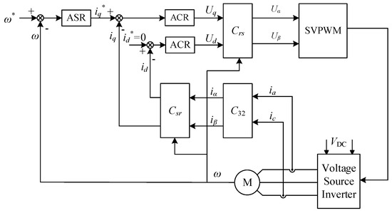
Figure 1.
Field-oriented control (FOC) of PMSM.
Here, M denotes PMSM, Csr is the transformation matrix from the αβ frame to the dq frame, and Crs is the inverse transformation matrix as follows:
where θ is the angle between the αβ and dq frames. Furthermore, C32 is the Clark transformation matrix and is expressed as follows:
To reduce costs, only two-phase currents should be sampled in the FOC algorithm because iA + iB + iC = 0. The remaining phase current can be then calculated. When sampling phase A and phase C currents, the currents in the αβ frame can be expressed as follows:
That is, the following expression is realized:
3. The 60° Coordinate System
The 60° coordinate system is always called the gh frame. The relationship between the gh and αβ frames is displayed in Figure 2.
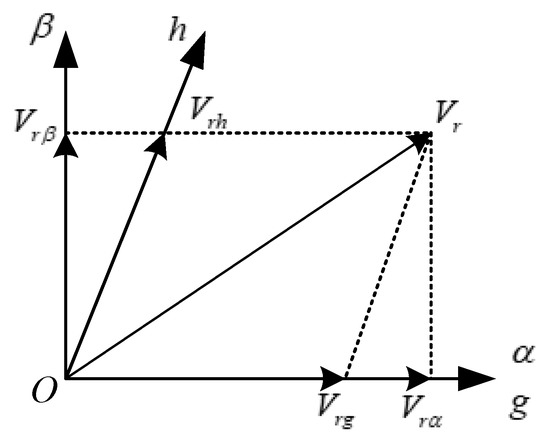
Figure 2.
Relationship between the and frames.
The relationship between the two coordinate systems is as follows:
The transformation matrix C is expressed as follows:
If the matrix is directly transformed from the three-phase coordinate system (abc frame) to the gh frame, the transformation matrix is D. The relationship is illustrated as follows:
The details of the transformation and characteristics of the 60° coordinate system are listed in the literature [24].
4. FOC Algorithm of the PMSM in the 60° Coordinate System
4.1. A. SVPWM Algorithm in the 60° Coordinate System
On implementing the SVPWM algorithm in a 60° coordinate system, the implementation process is simplified and the execution time of the algorithm is reduced. The SVPWM algorithm can be implemented using two techniques. In the first step, the sector judgment in which the reference voltage vector is located is performed. Next, the action time of basic voltage vectors is calculated. In the conventional orthogonal coordinate system, implementing these two steps is time-consuming. The characteristics of the 60° coordinate system simplify the implementation of these steps in the system. The voltage vectors and sector numbers in the 60° coordinate system are displayed in Figure 3 [24].
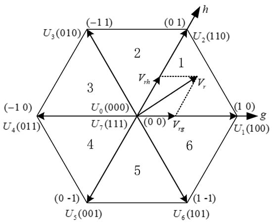
Figure 3.
Voltage vectors in the 60° coordinate system.
- (1)
- Sector judgment
The sector number in which the reference voltage vector is located can be obtained using the values of the g-axis component (Vrg) and h-axis component (Vrh) of the reference voltage vector (Vr) in the 60° coordinate system.
- ➢
- When Vrg + Vrh ≥ 0, the reference voltage vector is located in Sectors 1 or 2 or 6, then,
- (i)
- if Vrg < 0 → Sector 2;
- (ii)
- if Vrh < 0 → Sector 6;
- (iii)
- otherwise → Sector 1.
- ➢
- When Vrg + Vrh < 0, the reference voltage vector is located in Sectors 3 or 4 or 5, then,
- (i)
- if Vrh ≥ 0 → Sector 3;
- (ii)
- if Vrg ≥ 0 → Sector 5;
- (iii)
- otherwise → Sector 4.
- (2)
- Action time calculation
Determination of the sector in which the reference voltage vector is located facilitates the identification of basic voltage vectors selected to synthesize the reference vector. In the next step, the action time of basic voltage vectors is calculated. In the 60° coordinate system, the calculation process of the action time of the basic voltage vectors can be simplified to a certain extent.
Consider reference voltage vector Vr in Figure 3. The range of the g-axis component Vrg and h-axis component Vrh is (−1 to 1). When Vrg and Vrh are rounded up and down, four vectors can be obtained as follows [24]:
where subscripts U and L indicate rounding up and rounding down, respectively. While the reference voltage vector is located in Sector 1, the four vectors are illustrated in Figure 4.
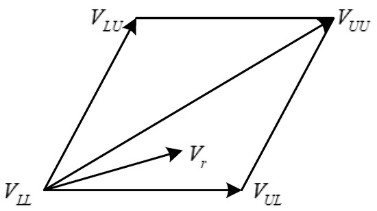
Figure 4.
Voltage vectors where the reference vector is rounded up and down.
According to voltage vector synthesis, the following expression can be obtained [24]:
where V1 = VUL, V2 = VLU, V3 = VLL, or V3 = VUU. When the reference voltage vector is located in Sectors 1, 3, and 5, V3 = VLL. When the reference voltage vector is located in Sectors 2, 4, and 6, V3 = VUU. Here, d1, d2, and d3 are the duty cycles of the basic vectors, which are used to synthesize the reference voltage vector.
When V3 = VLL, the action time can be calculated as follows [24]:
When V3 = VUU, the action time can be calculated as follows [24]:
The details of the SVPWM algorithm in the 60° coordinate system are illustrated in the literature [24]. When the SVPWM algorithm in the 60° coordinate system is applied in the conventional FOC, the structure of the system is displayed in Figure 5. The transformation matrix C should be added in front of the SVPWM.
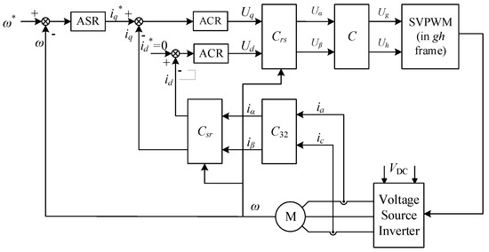
Figure 5.
FOC with the SVPWM in the 60° coordinate system.
4.2. FOC Structure of the PMSM in the 60° Coordinate System
The FOC structure of the PMSM in the 60° coordinate system is similar to that in the conventional orthogonal coordinate system. The structure diagram is displayed in Figure 6. Although the reference currents ig* and ih* are AC components, they are converted from the reference currents id* and iq* and their phases are determined by the rotor position, so it is also a field-oriented control structure (FOC).
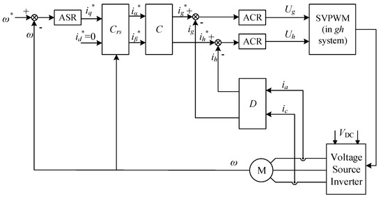
Figure 6.
FOC structure of the PMSM in the 60° coordinate system.
The structure of the current regulator in the 60° coordinate system is the same as that of the current regulator in the traditional FOC, both of which use the PI algorithm. Since the reference currents are AC components, compared with the traditional FOC, the proportional coefficient and the integral coefficient are adjusted, but the calculation burden of the processor will not be increased. One disadvantage is that due to the bandwidth limitation of the regulator, when the speed range of the motor is wide, the actual current and the reference current have amplitude and phase errors, which may affect the operation of the motor.
In Figure 6, the SVPWM algorithm is implemented in a 60° coordinate system. Another difference between the FOC in the 60° coordinate system and the conventional frame is that the reference currents ig* and ih* and feedback currents ig and ih are the values in the 60° coordinate system (Figure 6). The transformation matrixes C and D are already stated in Section 3.
The voltage equations of PMSM in the 60° coordinate system can be derived as follows:
where usg and ush are the g-axis and h-axis stator voltages, respectively; isg and ish are the g-axis and h-axis stator currents, respectively; ψsg and ψsh are g-axis and h-axis stator flux, respectively.
The expression of electromagnetic torque of the PMSM in the 60° coordinate system can be derived as follows:
FOC in the 60° coordinate system was studied to verify whether the algorithm can be simplified. The research results are realized by simulation and experiment.
5. Simulation Study
The FOC algorithms in the 60° coordinate system and conventional orthogonal coordinate system were simulated and compared in MATLAB/Simulink. The parameters of the PMSM and system are listed in Table 1, and the reference speed of the motor is set to 600 r/min in all the test states. Two test scenarios are set in which the motor is in an approximately no-load state and under-load state, respectively. When the motor is under load, the nature of the load is constant torque, and the magnitude is set to 0.8 Nm.

Table 1.
Motor and system parameters.
The three-phase current waveforms when the motor is in an approximately no-load state are illustrated in Figure 7. The three-phase current waveforms when the motor is under load are illustrated in Figure 8. The g-axis and h-axis currents of the motor are displayed in Figure 9. The reference current ig_ref and feedback current ig are illustrated in Figure 10.
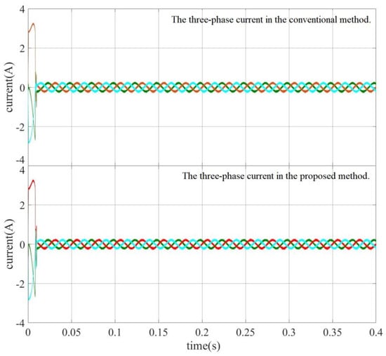
Figure 7.
Three-phase current waveforms when the motor is in an approximately no-load state.
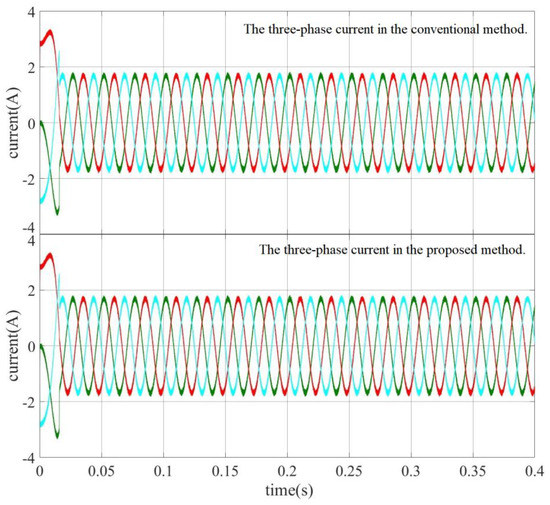
Figure 8.
Three-phase current waveforms when the motor is under load.
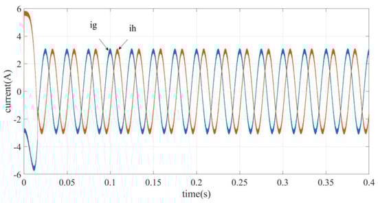
Figure 9.
The g-axis and h-axis currents when the motor is under load.
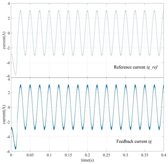
Figure 10.
Reference current ig_ref and feedback current ig.
The torque responses when the motor is in approximately a no-load state and under load are illustrated in Figure 11 and Figure 12, respectively. The speed responses are illustrated in Figure 13 and Figure 14.
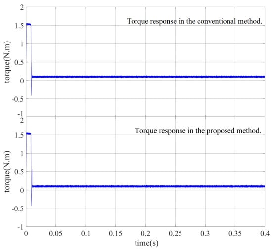
Figure 11.
Torque response when the motor is in the approximately no-load state.
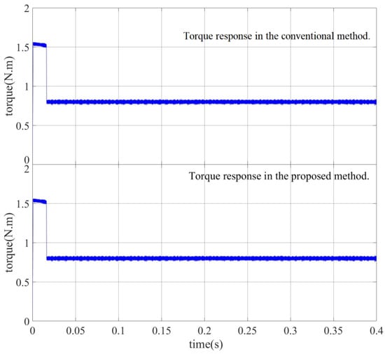
Figure 12.
Torque response when the motor is under load.
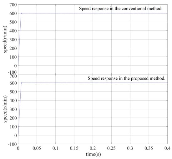
Figure 13.
Speed response when the motor is in an approximately no-load state.
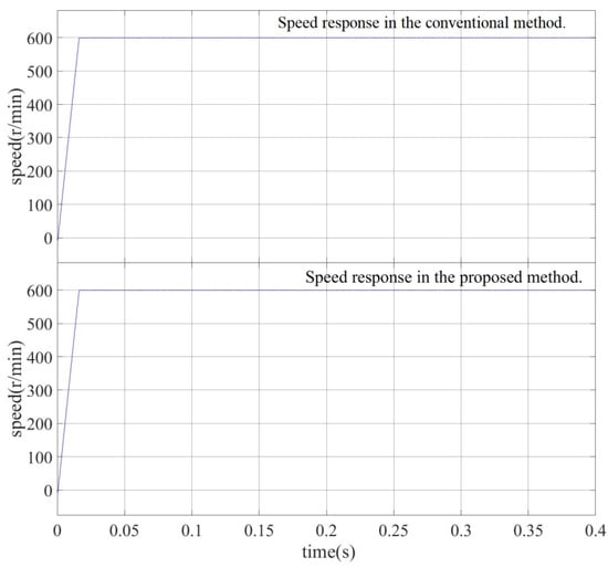
Figure 14.
Speed response when the motor is under load.
The motor response curves of the FOC algorithm in the 60° coordinate system are close to that of the FOC algorithm in the original orthogonal coordinate system. In the 60° coordinate system, the feedback currents are consistent with the reference currents. The simulation results validated the performance of the FOC algorithm in the 60° coordinate system.
6. Experimental Results
The simulation study in the MATLAB/Simulink environment illustrates the correctness of the algorithm implemented in a 60° coordinate system, but it could not detail the superiority compared with the original method. The algorithms should be studied in the environment of the hardware experiment. A 32-bit fixed-point DSP TMS320F2812 produced by Texas Instruments in America was used to realize the FOC algorithm in two coordinate systems, and the performances of the algorithm in the two systems were compared. The experimental setup is displayed in Figure 15. The parameters of the PMSM and control system are consistent with those parameters in the simulation environment (Table 1). The sampling frequency of the FOC algorithm in two coordinate systems is set to 10 kHz, and the system clock frequency is set to 150 MHz in all experimental tests.
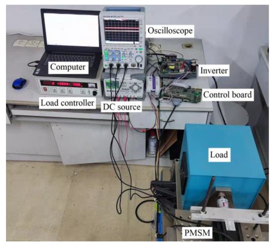
Figure 15.
Experimental setup of the two-level fed PMSM drive.
The code editing and compilation were implemented in the integrated development environment Code Composer Studio (CCS) version 6.1.3. The compiler version was C2000 V15.12.1. Comparing the compiled execution file revealed that the required memory for the conventional FOC and the FOC in the 60° coordinate system were 130 and 129 KB, respectively.
Comparing the FOC structure diagrams in Figure 1, Figure 5, and Figure 6 in the two coordinate systems revealed that they contained the following parts:
- (1)
- In the conventional orthogonal coordinate system: ASR, ACR, Crs, Csr, C32, and SVPWM.
- (2)
- In the 60° coordinate system: ASR, ACR, Crs, C, D, SVPWM in gh frame (SVPWM_gh).
The code execution time for some components need not be compared because of the same forms in the two frames. The same components include ASR, ACR, and Crs. The execution time of the code for the rest of the components should be carefully compared and analyzed. The code execution time of each link is tested using the clock calculation function in CCS. Breakpoints are set at the beginning and end of the code segment to calculate the number of clocks consumed in executing the code segment. The code execution time is displayed in Table 2:
Table 2.
Code execution time in two frames.
Comparing the code execution time of the corresponding links in the two coordinate systems revealed that the code execution time in the 60° coordinate system was reduced considerably. The main contribution to this result is the simplification of the SVPWM algorithm. Even though only the SVPWM algorithm is processed in the 60° coordinate system in the conventional FOC algorithm, where conversion module C should be added as displayed in Figure 5, the code execution time is also reduced.
In the 60° coordinate system, the code execution time of other transformation modules is reduced, especially the transformation matrix D. The cause of the reduction can be determined by observing Equation (9). By multiplying D by 3/2, the coefficient of 2/3 in Equation (9) can be removed, and the following expression can be obtained:
Due to , then
The values of the feedback currents in the 60° coordinate system ig and ih can be easily obtained by sampling the currents ia and ic (Figure 16). The reference current and feedback current in the 60° coordinate system are displayed in Figure 17. To transform the reference value in proportion to the feedback value, the transformation matrix C in Figure 6 should be multiplied by 3/2.
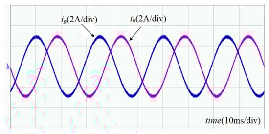
Figure 16.
g-axis and h-axis currents of the motor.
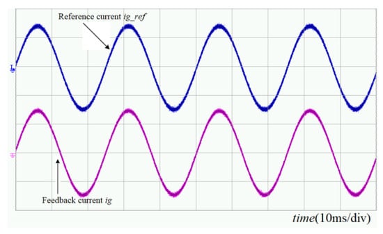
Figure 17.
Reference current ig_ref and feedback current ig of the motor.
Figure 18 and Figure 19 illustrate the current response and torque speed response, in which the upper curves correspond to the conventional coordinate system, and the lower curves correspond to the 60° coordinate system. The current response curve only reflects the steady state, and the torque and speed response curve includes the dynamics of the startup process. When the motor is in the no-load or load state, irrespective of whether it is the current response curve or the torque-speed response curve, the results of the FOC algorithm in the two coordinate systems are similar.
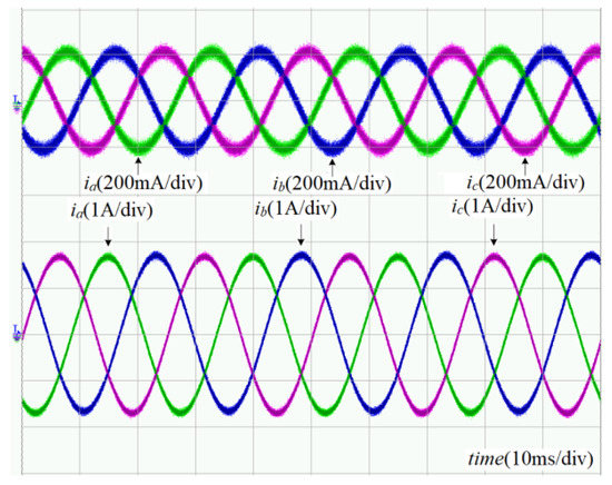
Figure 18.
Three-phase currents of the motor.
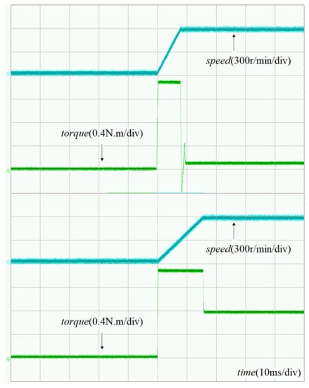
Figure 19.
Speed and torque responses of the motor.
The algorithm is implemented in the interrupt program, and the interrupt duration is 100 μs. To determine the algorithm execution time, an IO port of the processor is set to a low level at the beginning of the interrupt program, and the corresponding IO port is set to a high level at the end of the interrupt program. The low-level time of the IO port is observed through the oscilloscope, that is, the code execution time to be observed. The execution time test results are displayed in Figure 20, in which the waveform above corresponds to the conventional coordinate system, and the waveform below corresponds to the 60° coordinate system.
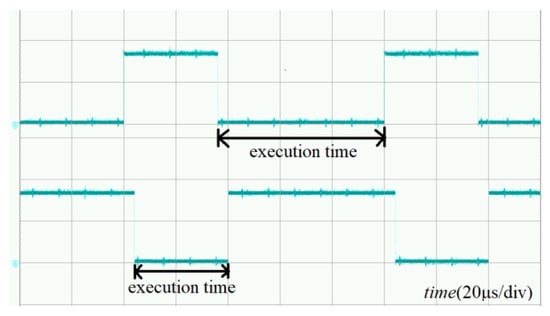
Figure 20.
Execution time of the code of the FOC algorithm in the DSP.
The experimental results revealed that the responses of the motor are similar when the FOC algorithm is performed in the conventional orthogonal coordinate system and in the 60° coordinate system. The execution time of the algorithm in the 60° coordinate system is shorter than that in the conventional orthogonal coordinate system. The execution time of the algorithm in the 60° coordinate system is approximately 38 μs while the execution time is approximately 64 μs in the conventional orthogonal coordinate system.
7. Conclusions
The FOC algorithm is a widely used and popular control strategy for PMSM. In this study, the FOC algorithm was implemented in the 60° coordinate system, and the feasibility of the FOC algorithm in the 60° coordinate system was verified by simulation analysis and experimental testing. The results revealed that the output performances of PMSMs in the 60° coordinate system are similar to those in the original orthogonal coordinate system. Comparing the code execution time revealed that the FOC algorithm of PMSM in the 60° coordinate system exhibits certain advantages. The shortening of the code execution time is conducive to the implementation of complex algorithms for PMSMs. Thus, this property is beneficial for applications at higher operating frequencies of devices, such as SiC. Another assistance is to use relatively cheaper processors to implement the FOC algorithm. Since the current controller uses the PI algorithm and it tracks AC current, the proposed method is not suitable for the motor to operate in a wide range of speed due to the limitation of the controller bandwidth. In the future, algorithms more suitable for AC current tracking control will be studied, such as the PR algorithm.
Author Contributions
Conceptualization, X.T.; formal analysis, X.T.; software, X.L. and C.L.; validation, Z.Z.; writing—original draft preparation, X.T.; writing—review and editing, M.J.; methodology, Y.S. All authors have read and agreed to the published version of the manuscript.
Funding
This study was supported in part by the Project of Guangdong Basic and Applied Basic Research Foundation (under Grant No. 2021A1515011563 and No. 2022A1515140009) and the Project of Dongguan Social Science and Technology Development (under Grant No. 2020507140141), in part by the Open Project of Hunan Provincial Key Laboratory of Artificial Intelligence for Medical Imaging (under Grant No. YXZN2022005) and Dongguan Sci-tech Commissioner Program (under Grant No. 20221800500242 and No. 20221800500072).
Institutional Review Board Statement
Not applicable.
Informed Consent Statement
Not applicable.
Conflicts of Interest
The authors declare no conflict of interest.
References
- Hu, W.; Nian, H.; Zheng, T. Torque ripple suppression method with reduced switching frequency for open-winding PMSM drives with common DC bus. IEEE Trans. Ind. Electron. 2019, 66, 674–684. [Google Scholar] [CrossRef]
- Pellegrino, G.; Vagati, A.; Guglielmi, P.; Boazzo, B. Performance comparison between surface-mounted and interior PM motor drives for electric vehicle application. IEEE Trans. Ind. Electron. 2012, 59, 803–811. [Google Scholar] [CrossRef]
- Ge, Y.; Yang, L.; Ma, X. Sensorless control of PMSM using generalized extended state observer and adaptive resistance estimation. IET Electr. Power Appl. 2020, 14, 2062–2073. [Google Scholar] [CrossRef]
- Domenico, C.; Francesco, P.; Giovanni, S.; Angelo, T. FOC and DTC: Two viable schemes for induction motor torque control. IEEE Trans. Power Electron. 2002, 17, 779–787. [Google Scholar]
- Lara, J.; Chandra, A. Performance investigation of two novel HSFSI demodulation algorithms for encoderless FOC of PMSMs intended for EV propulsion. IEEE Trans. Ind. Electron. 2018, 65, 803–811. [Google Scholar] [CrossRef]
- Wang, Z.; Chen, J.; Cheng, M.; Chau, K. Field-oriented control and direct torque control for paralleled VSIs fed PMSM drives with variable switching frequencies. IEEE Trans. Power Electron. 2016, 31, 2417–2428. [Google Scholar] [CrossRef]
- Wang, X.; Wang, Z.; Xu, Z.; Cheng, M.; Hu, Y. Optimization of torque tracking performance for direct torque controlled PMSM drives with composite torque regulator. IEEE Trans. Ind. Electron. 2020, 67, 10095–10108. [Google Scholar] [CrossRef]
- Heidari, R. Model predictive combined vector and direct torque control of SM-PMSM with MTPA and constant stator flux magnitude analysis in the stator flux reference frame. IET Electr. Power Appl. 2020, 14, 2283–2292. [Google Scholar] [CrossRef]
- Giuseppe, S.B.; Marian, P.K. Direct torque control of PWM inverter-fed AC motors—A survey. IEEE Trans. Ind. Electron. 2004, 51, 744–757. [Google Scholar]
- Zhang, Y.; Zhu, J. Direct torque control of permanent magnet synchronous motor with reduced torque ripple and commutation frequency. IEEE Trans. Power Electron. 2011, 26, 235–248. [Google Scholar] [CrossRef]
- Lara, J.; Xu, J.; Chandra, A. Effects of rotor position error in the performance of field-oriented-controlled PMSM drives for electric vehicle traction applications. IEEE Trans. Ind. Electron. 2016, 63, 4738–4751. [Google Scholar] [CrossRef]
- Alexandrou, A.D.; Adamopoulos, N.K.; Kladas, A.G. Development of a constant switching frequency deadbeat predictive control technique for field-oriented synchronous permanent-magnet motor drive. IEEE Trans. Ind. Electron. 2016, 63, 5167–5175. [Google Scholar] [CrossRef]
- Dusmez, S.; Qin, L.; Akin, B. A new SVPWM technique for DC negative rail current sensing at low speeds. IEEE Trans. Ind. Electron. 2015, 62, 826–831. [Google Scholar] [CrossRef]
- Zhang, L.; Fan, Y.; Cui, R.; Lorenz, R.D.; Cheng, M. Fault-tolerant direct torque control of five-phase FTFSCW-IPM motor based on analogous three-phase SVPWM for electric vehicle applications. IEEE Trans. Vehicular Tech. 2018, 67, 910–919. [Google Scholar] [CrossRef]
- Zhang, J.; Wai, R. Design of new SVPWM mechanism for three-level NPC ZSI via line-voltage coordinate system. IEEE Trans. Power Electron. 2020, 35, 8593–8606. [Google Scholar] [CrossRef]
- Krug, H.P.; Kume, T.; Swamy, M. Neutral-point clamped three-level general purpose inverter—Features, benefits and applications. In Proceedings of the 2004 IEEE 35th Annual Power Electronics Specialists Conference, Aachen, Germany, 20–25 June 2004. [Google Scholar]
- Gupta, A.K.; Khambadkone, A.M. A space vector PWM scheme for multilevel inverters based on two-level space vector PWM. IEEE Trans. Ind. Electron. 2006, 53, 1631–1639. [Google Scholar] [CrossRef]
- Holtz, J.; Oikonomou, N. Neutral point potential balancing algorithm at low modulation index for three-level inverter medium-voltage drives. IEEE Trans. Ind. Appl. 2007, 43, 761–768. [Google Scholar] [CrossRef]
- Celanovic, N.; Boroyevich, D. A fast space-vector modulation algorithm for multilevel three-phase converters. IEEE Trans. Ind. Appl. 2001, 37, 637–641. [Google Scholar] [CrossRef]
- Deng, Y.; Teo, K.H.; Duan, C.; Habetler, T.G.; Harley, R.G. A Fast and Generalized Space Vector Modulation Scheme for Multilevel Inverters. IEEE Trans. Power Electron. 2014, 29, 5204–5217. [Google Scholar] [CrossRef]
- Busquets-Monge, S.; Bordonau, J.; Boroyevich, D.; Somavilla, S. The nearest three virtual space vector PWM—A modulation for the comprehensive neutral-point balancing in the three-level NPC inverter. IEEE Power Electron. Letters 2004, 2, 11–15. [Google Scholar] [CrossRef]
- Lin, L.; Zou, Y.; Wang, Z.; Jin, H. Modeling and Control of Neutral-point Voltage Balancing Problem in Three-level NPC PWM Inverters. In Proceedings of the 2005 IEEE 36th Power Electronics Specialists Conference, Dresden, Germany, 16 June 2005. [Google Scholar]
- Lee, J.; Lee, K. Time-Offset Injection Method for Neutral-Point AC Ripple Voltage Reduction in a Three-Level Inverter. IEEE Trans. Power Electron. 2016, 31, 1931–1941. [Google Scholar] [CrossRef]
- Tang, X.; Yang, X.; Zhao, S.; Cao, J. Simulation of SVPWM overmodulation algorithm in 60-degree coordinate system. In Proceedings of the 2013 IEEE International Conference on Applied Superconductivity and Electromagnetic Devices, Beijing, China, 25–27 October 2013. [Google Scholar]
Disclaimer/Publisher’s Note: The statements, opinions and data contained in all publications are solely those of the individual author(s) and contributor(s) and not of MDPI and/or the editor(s). MDPI and/or the editor(s) disclaim responsibility for any injury to people or property resulting from any ideas, methods, instructions or products referred to in the content. |
© 2023 by the authors. Licensee MDPI, Basel, Switzerland. This article is an open access article distributed under the terms and conditions of the Creative Commons Attribution (CC BY) license (https://creativecommons.org/licenses/by/4.0/).