A Modeling and Control Algorithm for a Commercial Vehicle Electronic Brake System Based on Vertical Load Estimation

Abstract

In the electronic brake system (EBS) of commercial vehicles, due to the compressibility of gas, it is difficult to achieve accurate control in the pneumatic pipeline. To address this issue, a vertical load estimator based on unscented particle filtering (UPF) was designed, which can estimate vertical load during the running of the vehicle. Then, the EBS dynamics model was established based on software, including a brake signal sensor, single-channel bridge control module, ABS solenoid valve, and dual-channel bridge control module. Finally, based on the characteristics of the EBS valve, the control algorithm of the valve was studied, and the algorithm was tested using a hardware-in-the-loop experiment. The experiment results showed that the designed algorithm could improve braking performance.

1. Introduction

A commercial vehicle’s pneumatic braking transmission medium is compressed air, which has a certain hysteresis characteristic during the transmission process, resulting in a certain delay in the establishment and release of pressure in the braking pipeline, thereby affecting the braking efficiency of commercial vehicles. An electronic brake system (EBS) can effectively improve the stability of commercial vehicles. An EBS integrates components such as sensors, control units, and actuators.

Zhao et al. [1] proposed a practical hybrid model predictive controller based on an EBS. The controller is based on a simplified expression of system dynamics and considers the pressure variation caused by the switching state of the solenoid valve at the current and the last sampling time. Yang et al. [2] proposed a logic threshold control scheme based on an EBS that combines analog model predictive control and proportional control. Hamada et al. [3] conducted a comprehensive discussion on the basic principles of regenerative braking systems. In order to solve the problem of limited actuator response accuracy in EBSs, Shan et al. [4] proposed a control algorithm based on Q-learning to adjust the actuator commands. The traditional commercial vehicle electronic braking system has problems such as slow pressure response, large dynamic error, and unsatisfactory braking effect during the braking process. Zhang et al. [5] designed a new EBS system, which integrates the control of each pneumatic valve. Wu et al. [6] proposed a human–machine collaborative steering torque control method for intelligent vehicles. Yan et al. [7] proposed a lateral trajectory tracking strategy considering decision making based on the noncooperative Stackelberg equilibrium theory. Li et al. [8] proposed a dynamic coupled voltage regulation method for an EBS. Due to the switching characteristics of solenoid valves, it is difficult to ensure the precise pressure control and low switching activity of the valve during the braking process. To address this issue, Zhang et al. [9] proposed a hybrid model predictive control method to achieve multiobjective optimization, namely precise pressure tracking and reduced valve switching. Zhao et al. [10] proposed sliding mode control based on a safety distance strategy for the longitudinal control of truck platoons, and based on this, proposed an acceleration sliding mode controller. To improve driving comfort while ensuring braking safety, Bao et al. [11] studied the pressure change rate during the braking process using automatic pressure regulating valves as the research object. Zhao et al. [12] introduced the development and experimental verification of an electronically controlled pneumatic braking system controller based on model predictive control theory. In order to achieve precise pressure control for an EBS, Wu et al. [13] proposed a two-step nonlinear control strategy and designed a feasible controller. Yang et al. [14] used a combination of logic threshold control and phase plane theory to analyze the relationship between slip rate and braking torque during antilock braking, and obtained the composition law of the required braking torque for antilock braking. Slip rate control is crucial for improving vehicle stability and driving efficiency. Leng et al. [15] designed a robust slip rate control system for distributed drive electric vehicles. Han et al. [16] proposed a novel dual closed-loop cascade control structure for integrated electrohydraulic braking systems, which has the function of interconnecting pressure estimation. Xu et al. [17] proposed a motion decision algorithm based on Nash-Q learning that considers interaction. Zheng et al. [18] proposed a braking intention recognition algorithm suitable for commercial vehicles based on an EBS. Mishra et al. [19] proposed a novel nonlinear controller for the effective control of flow processes using viscous pneumatic control valves. Meng et al. [20] introduced system modeling and coupling analysis of a proportional solenoid valve with pulse width modulation control mode. Guo et al. [21] proposed an adaptive cruise control framework that considers regenerative braking. Santini et al. [22] proposed a new model-based technique for real-time road friction estimation under different environmental conditions. Hellgren et al. [23] proposed a calculation program to maximize regenerative braking energy during the braking process. Mosconi et al. [24] described the development of a vehicle state estimator aimed at real-time on-board use based on data collection already available in the vehicle CAN bus infrastructure. Chu et al. [25] used an unscented particle filter to estimate tire lateral force, longitudinal velocity, lateral velocity, and yaw rate. The estimator proposed by Wang et al. [26] consists of a lower layer and an upper layer, where a particle filter is applied to complete the estimation. Lui et al. [27] studied the ability of deep neural networks to predict missile maneuvering trajectories. Zhang et al. [28] proposed a state estimation method based on an enhanced adaptive unscented Kalman filter. Liu et al. [29] proposed a modular comprehensive estimation algorithm for the longitudinal and lateral states of the front vehicle. However, none of the above studies considered the structured modeling of the EBS.

Compared with previous studies, the main contributions of this study are as follows:

(1)

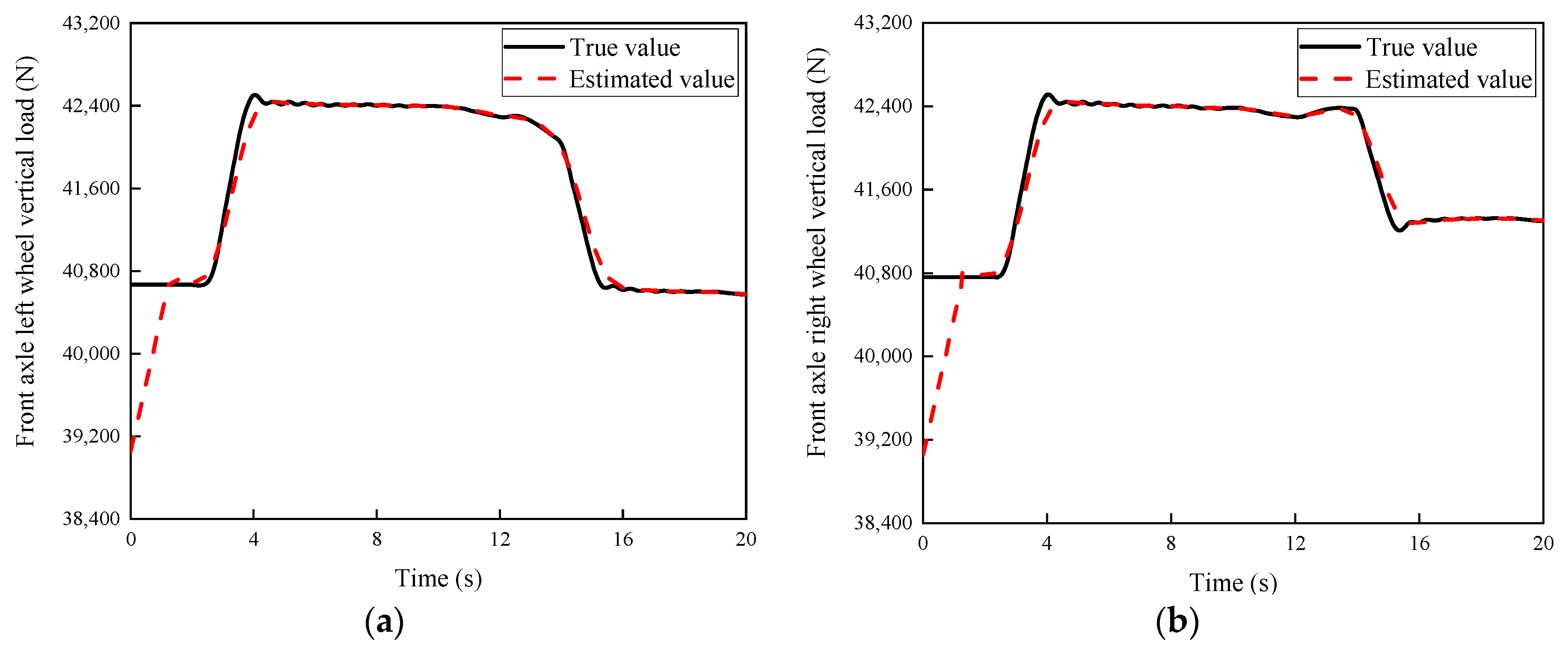
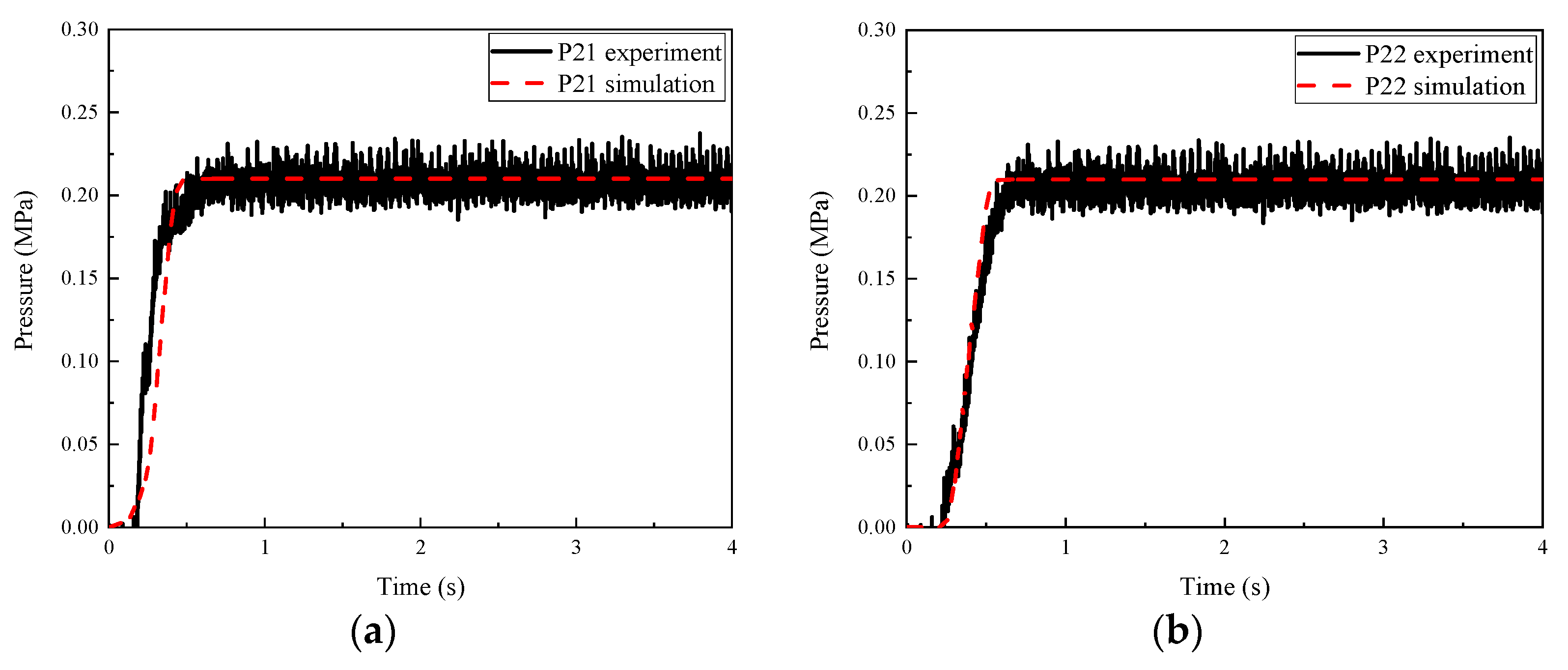
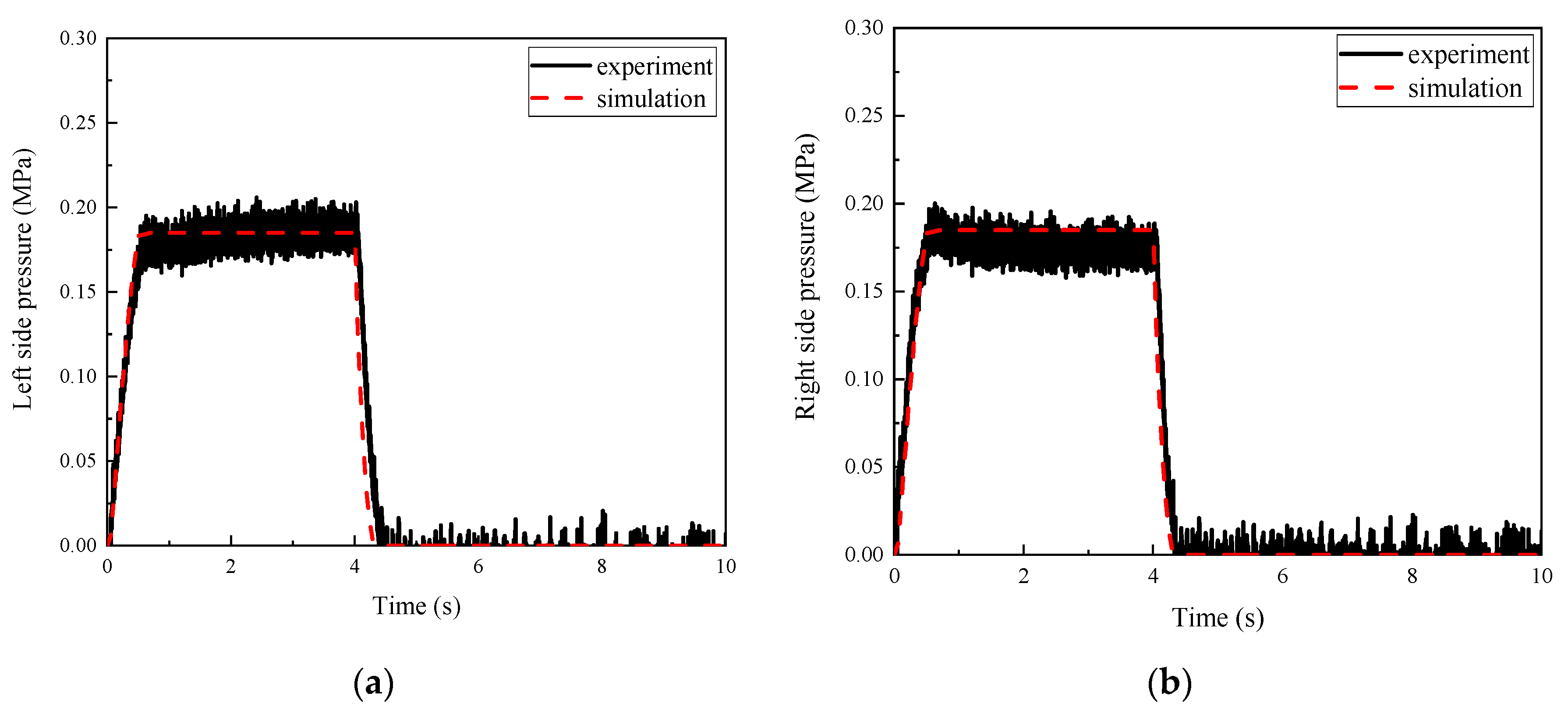
The designed vertical load estimation algorithm based on unscented particle filtering (UPF) is validated through simulation and can accurately estimate the vertical load of wheels. In order to study the gas transmission of an EBS more accurately, an EBS valve model is established.

(2)

A commercial vehicle EBS control algorithm is proposed to achieve better braking performance, which includes a vertical load estimation and a valve control algorithm.

The study is arranged as follows: The vertical load estimation algorithm is proposed in Section 2. The modeling of a commercial vehicle EBS is introduced in Section 3. The commercial vehicle EBS control algorithm is introduced in Section 4. The hardware-in-the-loop experimental verification of the commercial vehicle EBS control algorithm is conducted in Section 5. The summary is presented in Section 6.

2. Vertical Load Estimation

The particle filter algorithm can be applied to nonlinear systems and provide more accurate state estimation results. Therefore, this study proposes a wheel vertical load estimation algorithm based on UPF.

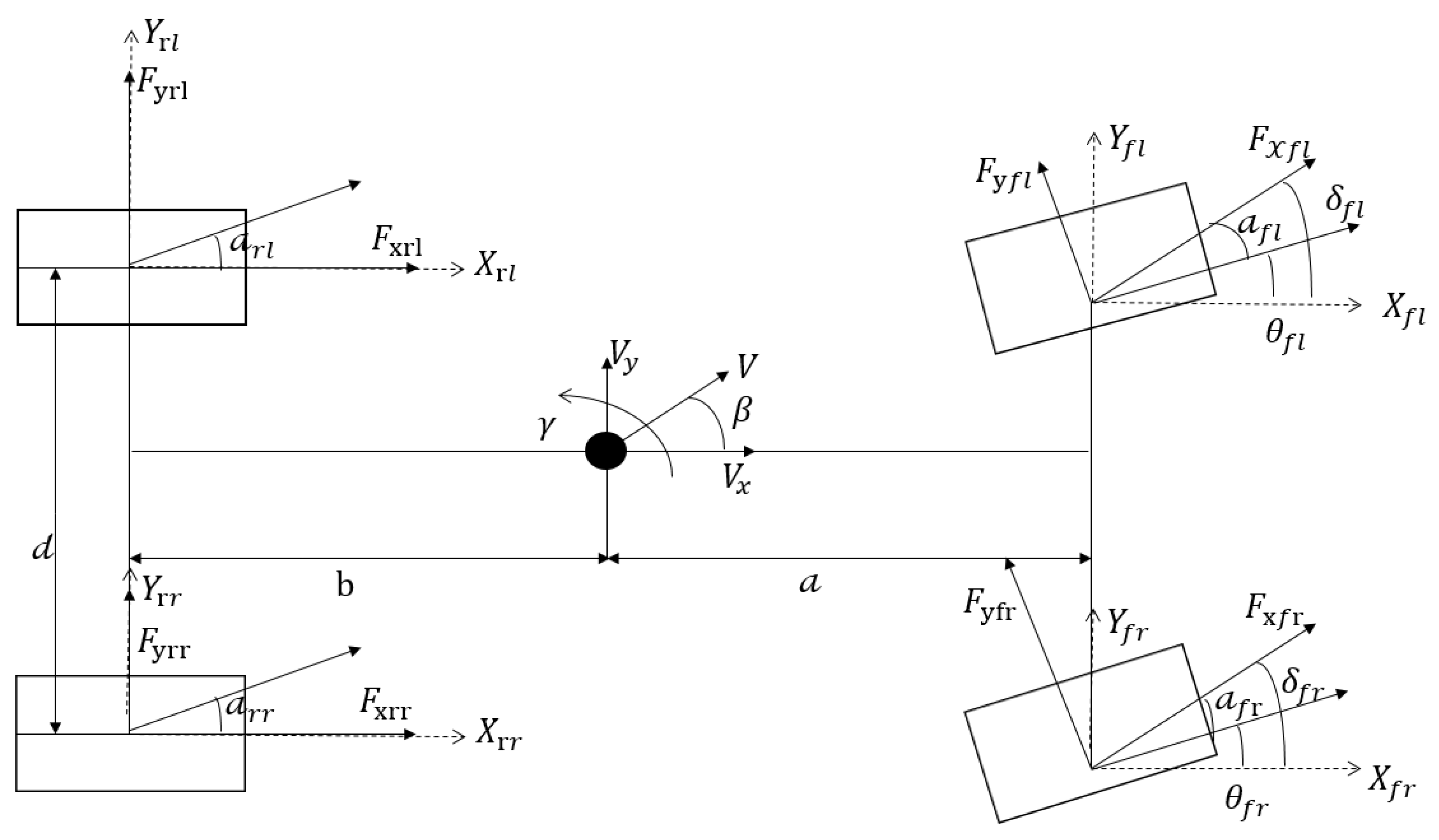
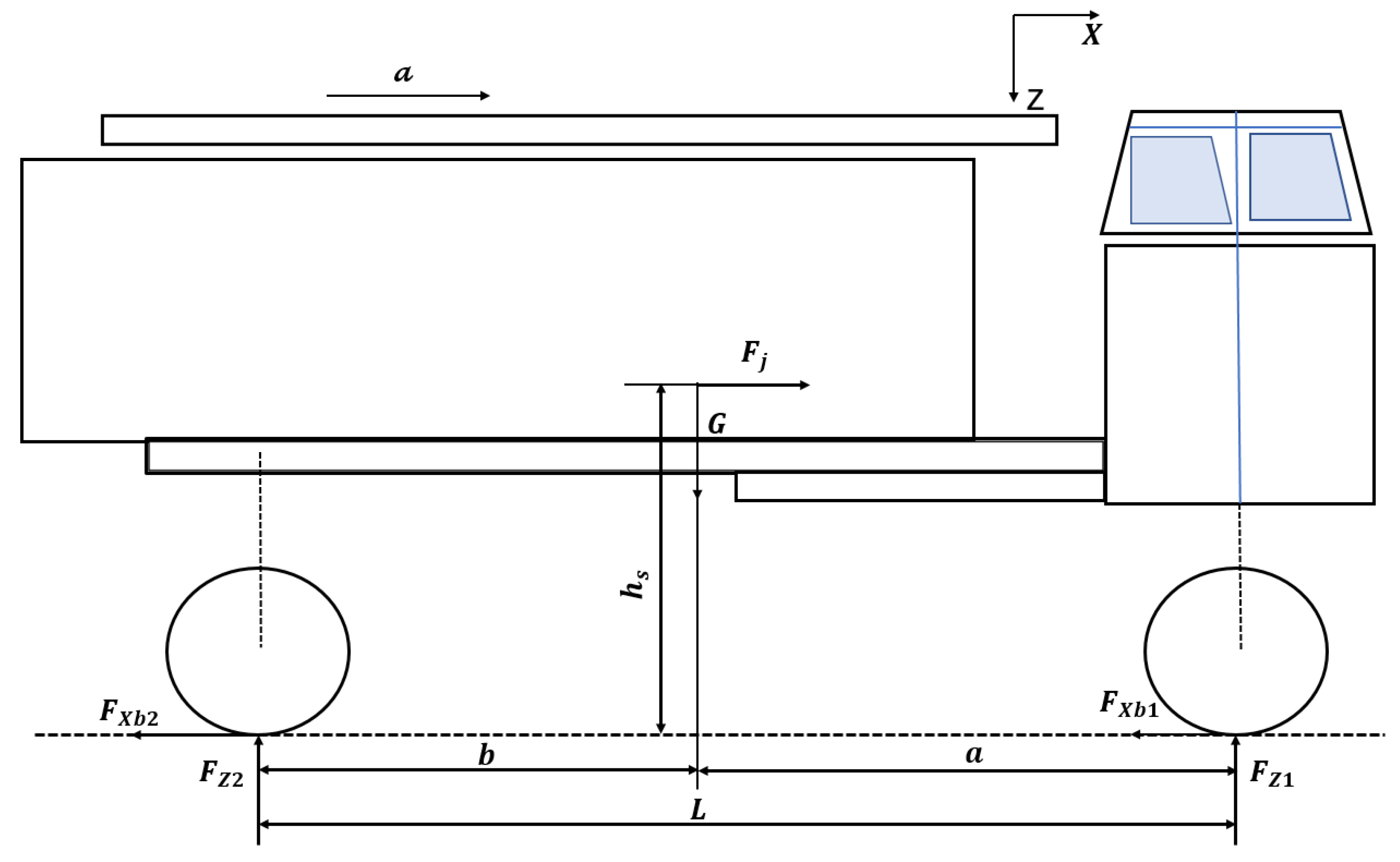
2.1. Commercial Vehicle Dynamics Model

This study involves the equivalent transformation of the three-axle vehicle model into a simplified two-axle vehicle model. As shown in Figure 1, ${\delta }_{ij}$ is the wheel angle. $i$ can be $l$ or $r$, representing the left or right wheel. $j$ can be $f$ or $r$, representing front or rear axle. $F_{xij}$ and $F_{yij}$ are the longitudinal and lateral forces of the wheels. $X_{ij}$ and $Y_{ij}$ are the longitudinal and lateral component forces of the wheel.

The force exerted by the vehicle in the horizontal (x) direction is represented by Equation (1).

$$X_{ij}=\cos {\delta }_{ij}{F}_{xij}-\sin {\delta }_{ij}{F}_{yij}$$

(1)

The aerodynamic drag experienced by the vehicle is expressed through Equation (2).

$$F_d=\frac{1}{2}\rho C_{d}A{v}_x^2$$

(2)

where $\rho$ represents the air density, $C_d$ is the wind resistance coefficient, $A$ is the contact area, and $v_x$ is the longitudinal speed of the vehicle.

The longitudinal acceleration of the vehicle is represented by Formula (3).

$$m{a}_x={\displaystyle {\sum }_{i=l}^r{\displaystyle {\sum }_{j=f}^r{X}_{ij}}}-F_d$$

(3)

The vertical load of the wheel is represented by Formula (4).

$$\begin{array}{l}{F}_{zlf}=\frac{mg{l}_r}{2(l_f+l_r)}-\frac{m_s{a}_x{h}_s}{2(l_f+l_r)}-\frac{m_s{a}_y{h}_s}{t_f}\\ F_{zrf}=\frac{mg{l}_r}{2(l_f+l_r)}-\frac{m_s{a}_x{h}_s}{2(l_f+l_r)}+\frac{m_s{a}_y{h}_s}{t_f}\\ F_{zlr}=\frac{mg{l}_f}{2(l_f+l_r)}+\frac{m_s{a}_x{h}_s}{2(l_f+l_r)}-\frac{m_s{a}_y{h}_s}{t_r}\\ F_{zrr}=\frac{mg{l}_f}{2(l_f+l_r)}+\frac{m_s{a}_x{h}_s}{2(l_f+l_r)}+\frac{m_s{a}_y{h}_s}{t_r}\end{array}$$

(4)

where $F_{zlf}$ and $F_{zrf}$, respectively, represent the vertical load of the left and right wheels on the front axle of the vehicle; $F_{zlr}$ and $F_{zrr}$, respectively, represent the vertical load of the left and right wheels on the rear axle of the vehicle; $l_f$ and $l_r$, respectively, represent the front wheelbase and rear wheelbase of the vehicle; $m_s$ represents the spring loaded mass; and $h_s$ represents the height from the center of the sprung mass to the ground, as shown in

Table 1. (a) Vehicle dynamics parameter list; (b) Vehicle parameters.

(a)
Symbol	Meaning
${\delta }_{lf}$	the left wheel angle of the front axle
${\delta }_{rf}$	the right wheel angle of the front axle
${\delta }_{lr}$	the left wheel angle of the rear axle
${\delta }_{rr}$	the right wheel angle of the rear axle
$F_{xlf}$	the longitudinal forces on the left wheel of the front axle
$F_{xrf}$	the longitudinal forces on the right wheel of the front axle
$F_{xlr}$	the longitudinal forces on the right wheel of the rear axle
$F_{xrr}$	the longitudinal forces on the right wheel of the rear axle
$F_{ylf}$	the lateral forces on the left wheel of the front axle
$F_{yrf}$	the lateral forces on the right wheel of the front axle
$F_{ylr}$	the lateral forces on the left wheel of the rear axle
$F_{yrr}$	the lateral forces on the right wheel of the rear axle
$X_{lf}$	the longitudinal component forces on the left wheel of the front axle
$X_{rf}$	the longitudinal component forces on the right wheel of the front axle
$X_{lr}$	the longitudinal component forces on the left wheel of the rear axle
$X_{rr}$	the longitudinal component forces on the right wheel of the rear axle
$Y_{lf}$	the lateral component forces on the left wheel of the front axle
$Y_{rf}$	the lateral component forces on the right wheel of the front axle
$Y_{lr}$	the lateral component forces on the left wheel of the rear axle
$Y_{rr}$	the lateral component forces on the right wheel of the rear axle
$\rho$	the air density
$C_d$	the wind resistance coefficient
$A$	the contact area
$v_x$	the longitudinal speed of the vehicle
$F_{zlf}$	the vertical load of the left wheels on the front axle
$F_{zrf}$	the vertical load of the right wheels on the front axle
$F_{zlr}$	the vertical load of the left wheels on the rear axle
$F_{zrr}$	the vertical load of the right wheels on the rear axle
$l_f$	the front wheelbase of the vehicle
$l_r$	the rear wheelbase of the vehicle
$m_s$	the spring-loaded mass
$h_s$	the height from the center of the sprung mass to the ground
(b)
Parameter		Value	Unit
Unloaded sprung mass		4450	kg
Fully loaded sprung mass		10,000	kg
Centroid height		1.175	m
Tread		2.03	m
Wheel radius		510	mm
$\rho$		1.2258	N × s2 × m−4
$C_d$		0.3	/
$A$		7.125	m2

.

2.2. Vertical Load Estimation Based on Unscented Particle Filter

The primary benefit of the unscented particle filter (UPF) lies in its capability to effectively address nonlinearity in systems while circumventing the issue of sample degradation encountered in conventional studying filtering methodologies. Therefore, this study used the unscented particle filter algorithm to estimate the vertical load of the wheels.

In accordance with the chosen vehicular model, this investigation employed the longitudinal acceleration of the vehicle and the vertical load distribution on both the front and rear axles as the state variables, as depicted in Equation (5).

$$X=[a_x{F}_{zlf}{F}_{zrf}{F}_{zlr}{F}_{zrr}]$$

(5)

We considered the wheel’s vertical load accompanied by Gaussian noise and the corresponding output variables of the commercial vehicle transmission system model as observed measurements, as indicated in Equation (6).

$$Z=[F_{zlf}{}^{\prime }{F}_{zrf}{}^{\prime }{F}_{zlr}{}^{\prime }{F}_{zrr}{}^{\prime }Y]$$

(6)

Figure 2 shows a longitudinal force diagram of commercial vehicles.

There is a linear relationship between the torque, external force, and engine speed of commercial vehicle engines, as shown in Formulas (7)–(10).

$$y=M_c{K}_g-{\omega }_w[J_f+J_w+K_g{}^2(J_g+J_e)]-F_d{r}_w$$

(7)

$$y=[r_w^2{\omega }_w+r_w(g\sin \chi +c_{r1})]m=k_{y}m$$

(8)

$$K_g=K_{gt}{K}_{gf}$$

(9)

$$Y=M_c{K}_g-{\omega }_w[J_f+J_w+K_g{}^2(J_g+J_e)]-F_d{r}_w$$

(10)

where $M_c$ is the combustion torque generated by internal friction compensation in the engine, $K_{gt}$ is the transmission ratio, $K_{gf}$ is the transmission ratio of the final drive, ${\omega }_w$ is the wheel speed, $J_f$ is the rotational inertia of the main reducer, $J_w$ is the moment of inertia of the wheel, $J_g$ is the rotational inertia of the transmission, $J_e$ is the moment of inertia of the engine, $F_d$ is the air resistance, $r_w$ is the rolling radius of the wheel, $\chi$ is the slope of the road, and $c_{r1}$ is the tire parameter.

The input signal utilized by this state estimator is depicted in Equation (11).

$$u=[F_x{F}_y{\delta }_{ij}{\omega }_{ij}]$$

(11)

The discretized representation of the system is illustrated by Equations (12) and (13).

$$x(k+1)=f[x(k),u(k)]+Q(k)$$

(12)

$$y(k)=Hx+R(k)$$

(13)

where $H$ is a coefficient matrix.

$$H=\left[\begin{array}{cccc}0& 1& 0& 0\\ 0& 0& 1& 0\\ 0& 0& 0& 1\\ \begin{array}{l}0\\ 0\end{array}& \begin{array}{l}0\\ 0\end{array}& \begin{array}{l}0\\ 0\end{array}& \begin{array}{l}0\\ 0\end{array}\end{array}\begin{array}{c}0\\ 0\\ 0\\ \begin{array}{l}1\\ 0\end{array}\end{array}\begin{array}{c}0\\ 0\\ \begin{array}{l}0\\ 0\end{array}\\ k_y\end{array}\right]$$

(14)

$Q$ and $R$ represent process noise and measurement noise, respectively, both of which are diagonal matrices.

Firstly, N particle were extracted and initial values $x^{(i)}(0)$ and $p^{(i)}(0)$ were assigned to their state variables and covariance.

$${\overline{x}}^{(i)}(0)=E[x^{(i)}(0)]$$

(15)

Afterwards, the pstudies were normalized.

$$x^{(i)a}(k-1)={\left[\begin{array}{c}{\overline{x}}^{(i)a}(k-1)\\ {\overline{x}}^{(i)a}(k-1)+\sqrt{(n+\lambda )p^{(i)a}(k-1)}\\ {\overline{x}}^{(i)a}(k-1)-\sqrt{(n+\lambda )p^{(i)a}(k-1)}\end{array}\right]}^T$$

(16)

where

$$\lambda ={\alpha }^2(n+\kappa )-n$$

(17)

The weight coefficient was defined as follows.

$$\{\begin{array}{c}{W}_0^{(m)}=\frac{\lambda }{N_x+\lambda }\\ W_i^{(m)}=\frac{\lambda }{2(N_x+\lambda )}\end{array}$$

(18)

$$\{\begin{array}{c}{W}_0^{(c)}=\frac{\lambda }{N_x+\lambda }+(1-{\alpha }^2+\beta )\\ W_i^{(c)}=\frac{\lambda }{2(N_x+\lambda )}\end{array}$$

(19)

where $N_x$ is the number of state variables.

Next, the state of the studied system was updated based on the aforementioned model.

$$x^{(i)x}(k|k-1)=f(x^{(i)x}(k-1),u(k-1))$$

(20)

$${\overline{x}}^{(i)x}(k|k-1)={\displaystyle {\sum }_{j=0}^{2n}{W}_j^{(m)}}{x}_j^{(i)x}(k|k-1)$$

(21)

Afterwards, the state estimation value was calculated based on the weight coefficients and particle state values.

The output value of the system was updated.

$${\overline{y}}^{(i)}(k|k-1)={\displaystyle {\sum }_{j=0}^{2n}{W}_j^{(m)}}{y}_j^{(i)x}(k|k-1)$$

(22)

The revised covariance matrix is presented below.

$$X_{\overline{x}}=x_j^{(i)x}(k|k-1)-{\overline{x}}^{(i)}(k|k-1)$$

(23)

$$P_{(X,X)}^{(i)}(k|k-1)={\displaystyle {\sum }_{j=0}^{2n}{W}_j^{(c)}}{X}_{\overline{x}}{X}_{\overline{x}}{}^T$$

(24)

The Kalman filter gain is as follows:

$$K(k)=P_{(x,y)}(k){[P_{(y,y)}]}^{-1}$$

(25)

Therefore, the posterior estimation and posterior covariance are as follows:

$${\overline{x}}^{(i)}(k)={\overline{x}}^{(i)}(k|k-1)+K(k)[y(k)-{\overline{y}}^{(i)}(k|k-1)]$$

(26)

$${\widehat{P}}^{(i)}(k)=P_{(x,x)}^{(i)}(k|k-1)-K(k)P_{(y,y)}(k){[K(k)]}^{-1}$$

(27)

After undergoing multiple iterations, the degradation of particles occurs due to the impact of weight factors, leading to ineffective updates. Consequently, resampling becomes imperative to assign appropriate weight coefficients to each particle.

$${\omega }^{(i)}(k)=1/N$$

(28)

$${\overline{x}}^{(i)}(k)={\displaystyle {\sum }_{i=1}^N{\omega }^{(i)}(k){\overline{x}}^{(i)}(k)}$$

(29)

$${\widehat{P}}^{(i)}(k)={\displaystyle {\sum }_{i=1}^N{\omega }^{(i)}}(k)[x^{(i)}(k)-{\overline{x}}^{(i)}(k)]{[x^{(i)}(k)-{\overline{x}}^{(i)}(k)]}^T$$

(30)

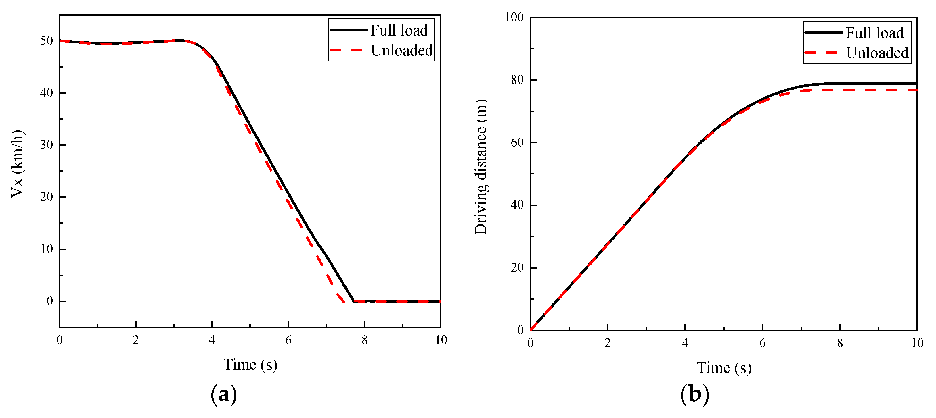
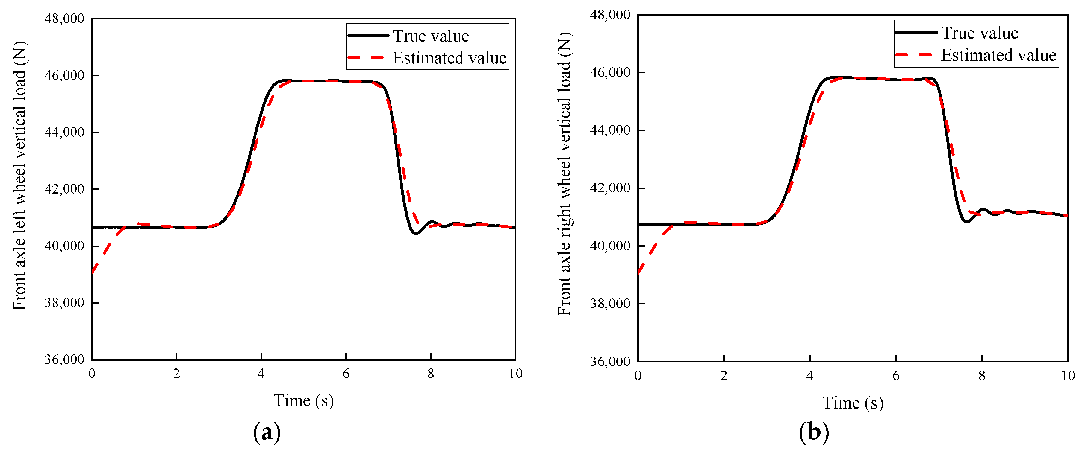
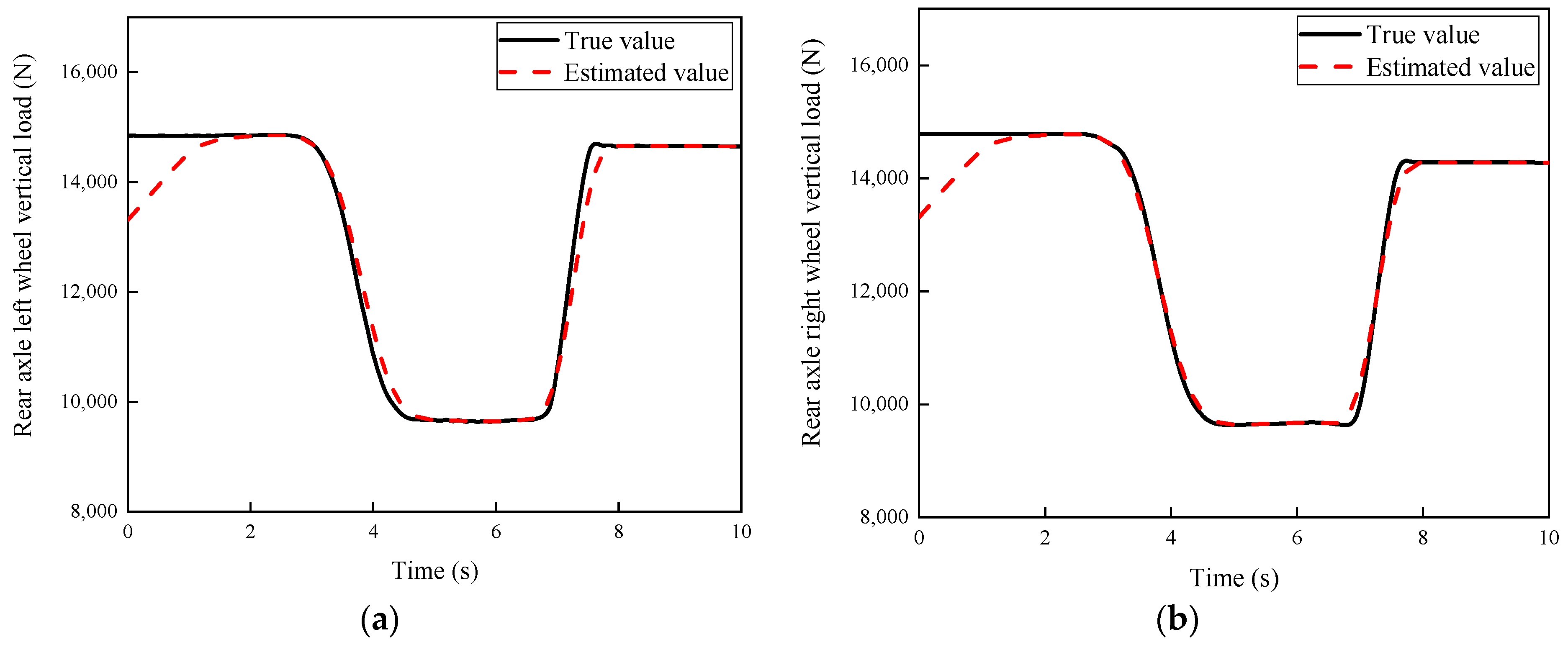
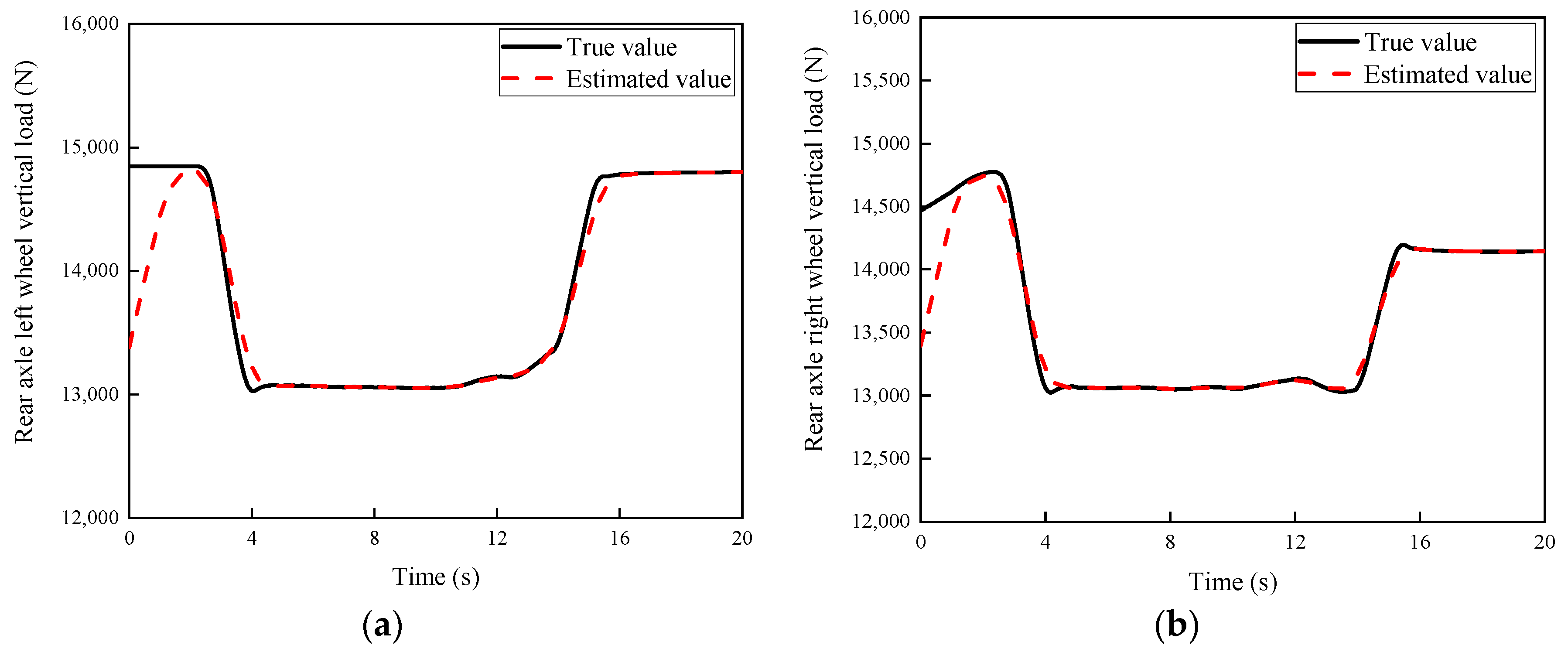
2.3. Simulation Verification

In order to validate the efficacy of the proposed wheel load estimator, comprehensive simulation tests were conducted on the simulation platform, considering two representative operational scenarios: high attachment with full load brake and low attachment with full load brake.

The road adhesion coefficient is 0.85. The vehicle is in a fully loaded state. The vehicle is operated at a constant velocity prior to the initiation of the braking procedure. It can be seen in Figure 3 and Figure 4. The initial values of the vehicle load estimation algorithm are preset as 39,057 N for the front axle and 13,312 N for the rear axle. At 0 s, there is an error between the estimated vehicle load and the actual value. At around 0 to 1.12 s, the estimated vehicle load converges to the true value. At the onset of braking at 3 s, the vehicle experiences forward movement of its center of mass, leading to an increase in the load on the front axle and a decrease in the load on the rear axle.

The road adhesion coefficient is 0.23. The vehicle is in a fully loaded state. The vehicle is driven at a uniform speed before braking. It can be seen in Figure 5 and Figure 6. Due to the preset initial values of the vehicle load estimation algorithm being 39,057 N for the front axle and 13,312 N for the rear axle, at the initial moment (0 s), a discrepancy is observed between the estimated vehicle load and the actual value. The estimated vehicle load gradually approaches convergence with the true value within the time interval of 0 to 1.21 s. Subsequently, at 3 s, the vehicle initiates the braking process, resulting in a forward displacement of the vehicle’s center of mass. This displacement causes an elevation in the load exerted on the front axle, accompanied by a simultaneous reduction in the load on the rear axle.

3. Commercial Vehicle EBS Modeling

On the basis of analyzing the basic working principles of various components of EBS, in order to ensure the control accuracy of the EBS algorithm, this study considered that EBS is an integrated system of mechanics, electricity, and gas, and establish a commercial vehicle EBS dynamic model. The EBS configuration employed in this investigation comprises a brake signal sensor integrated into the brake pedal, a single-channel bridge control module responsible for the front axle, two ABS solenoid valves, and a dual-channel bridge control module dedicated to the rear axle.

3.1. Working Principle and Modeling of Brake Signal Sensors

The brake signal sensor acquires and transmits the brake pedal signal to the electronic control unit (ECU) for the purpose of analyzing the driver’s intended actions. Simultaneously, the brake signal sensor assumes a critical role within the pneumatic control circuit, incorporating an internal dual-redundant air circuit structure to uphold the stability of the braking system. The brake signal sensor will send a certain signal value in real time to the central ECU of the vehicle during normal driving, including a positive-slope signal, a negative-slope signal, and a step signal. In this context, the positive-slope signal and negative-slope signal exhibit a linear correlation with the degree of brake pedal opening. Conversely, the step signal primarily reflects the activation status of the brake pedal while also accounting for the idle travel of the brake pedal. In addition, according to the static characteristic curve of the brake pedal opening and output pressure, the brake signal sensor will also output the corresponding pressure. In the event of an electronic control circuit malfunction, this pressure can serve as an alternative pressure source to support the operation of other modules as a backup measure.

As shown in Figure 7, in the pneumatic circuit of the brake signal sensor: Port 11 is the air inlet for the brake signal sensor and is connected to the air reservoir. Port 21 is the air outlet and is connected to the front-axle single-channel bridge control module. Port 22 is also an air outlet, connected to the rear-axle dual-channel bridge control module. Port 3 signifies exhaust ports which are connected to the atmosphere. Within the electronic control circuit, port 1 and port 2 serve as power supply connections responsible for providing voltage to the brake signal sensor. Port 4 is designated as a positive-slope voltage output port, indicating a proportional relationship between the output voltage and the degree of pedal opening. Correspondingly, port 5 functions as a negative-slope voltage output port, with the output voltage displaying an inverse correlation with the pedal opening. Lastly, port 6 serves as the output port for the step signal, characterized by two distinct voltage values denoting the triggered and not-triggered states of the pedal.

Based on the working principle of the brake signal sensor, a brake signal sensor model as shown in Figure 8 was developed.

The output pressures of ports 21 and 22 are shown in Figure 9 for when the gas source pressure is 0.2 MPa.

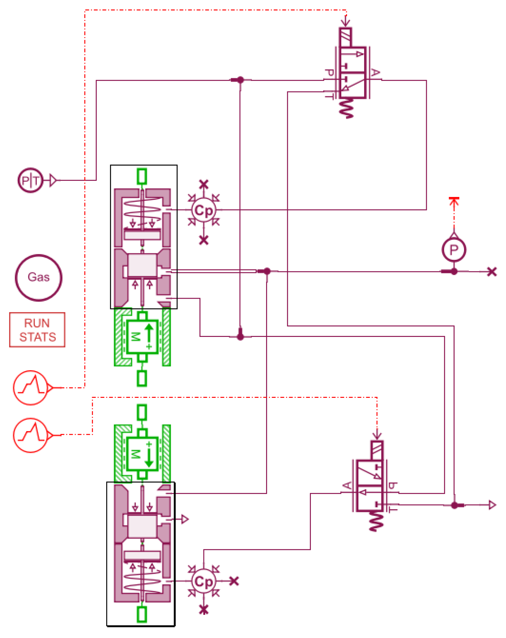
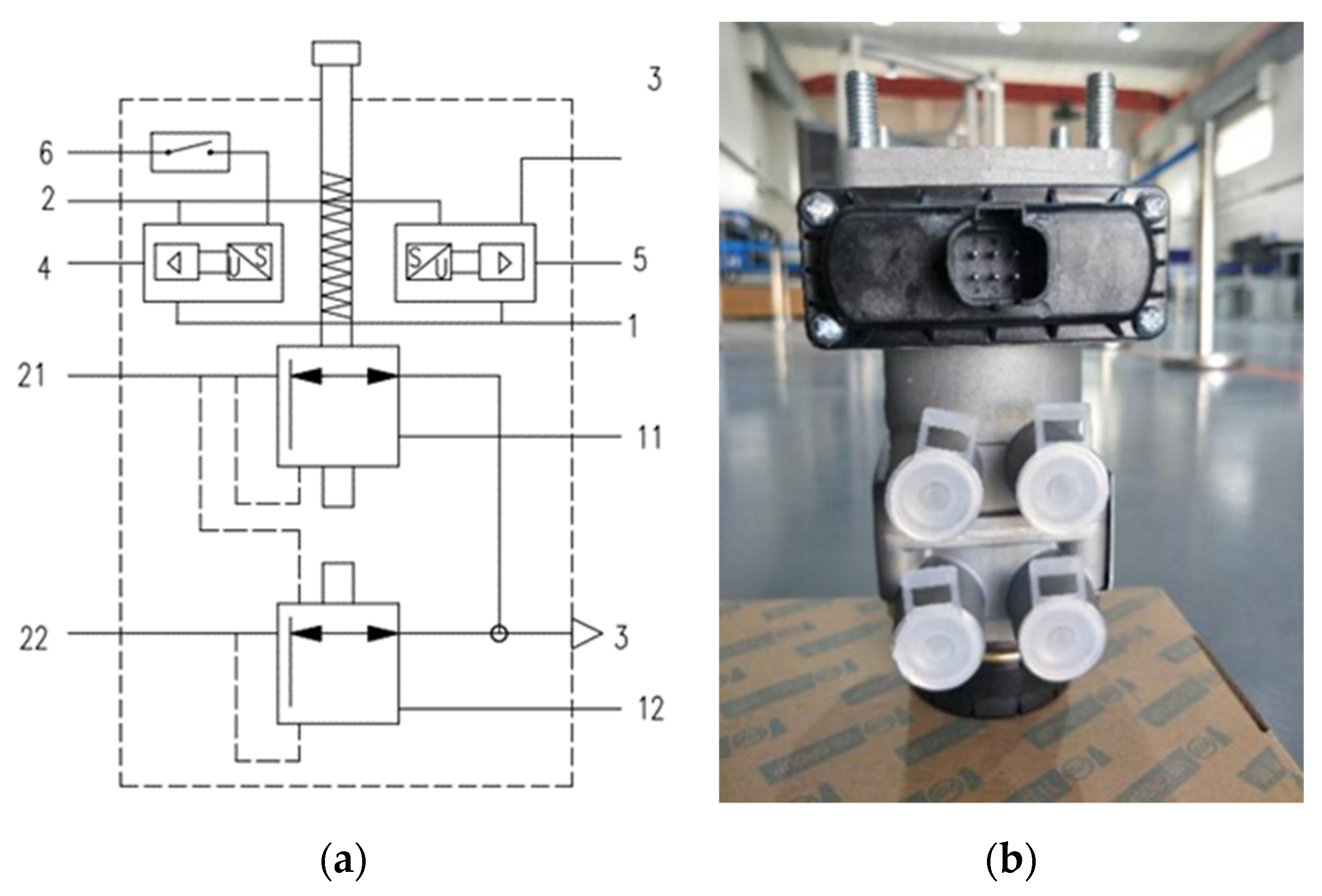
3.2. Working Principle and Modeling of Single-Channel Bridge Control Module

Currently, in the automotive industry, the front axle of vehicles commonly employs a monolithic bridge control module for pressure regulation. This module primarily consists of a boost valve, a pressure reduction valve, and a fail-safe valve.

In Figure 10, the working principle diagram and physical diagram of the single-channel bridge control module are shown, respectively. During typical vehicle operation, the single-channel bridge control module receives signals from the central electronic control unit (ECU) and regulates the output port pressure by means of the internal boost valve and pressure-reducing valve, aiming to achieve the desired pressure value. When the electronic control fails, the backup valve is used to enable the vehicle to brake normally and improve driving safety.

As shown in Figure 10, in the pneumatic circuit of the single-channel bridge control module: Port 1 is the air inlet and is connected to the air storage cylinder. Port 2 signifies air outlets connected to the ABS solenoid valve. Port 3 corresponds to the exhaust ports, which are effectively vented to the surrounding atmosphere. Port 4 serves as the control port, responsible for regulating the valve’s operation. In the event of an electronic control circuit malfunction, the valve seamlessly transitions to pneumatic control, ensuring its continued functionality.

During regular vehicle operation, the boost solenoid valve remains in a de-energized state, while both the pressure-reducing solenoid valve and the backup solenoid valve are also powered off. However, when engaging the braking system, specifically during the boost phase, the boost solenoid valve is activated, the pressure-reducing solenoid valve is deactivated, and the backup solenoid valve is subsequently energized. Gas enters the brake chamber from the air reservoir through a single-channel bridge control module and pneumatic pipeline. In the pressure-reducing stage, the boost solenoid valve is powered off, the pressure-reducing solenoid valve is powered on, and the backup solenoid valve is powered on. The ingress of gas from the air reservoir into the brake chamber is prevented, while the gas present in the brake chamber is discharged into the atmosphere via the exhaust port, thereby facilitating the pressure reduction process. In the pressure-maintaining stage, the boost solenoid valve is powered off, the pressure-reducing solenoid valve is powered off, and the backup solenoid valve is powered on. The airflow originating from the air reservoir is effectively prevented from entering the brake chamber, while simultaneously ensuring that the gas within the brake chamber remains undischarged. This outcome is instrumental in achieving the desired pressure maintenance effect. The operational attributes of the single-channel bridge control module, as described in the aforementioned procedure, are summarized in

Table 2. Operating characteristics of single-channel bridge control module.

	Boost Valve	Pressure-Reducing Valve	Backup Valve
Boosting	power on	power outage	power on
Reduce pressure	power outage	power on	power on
Maintaining pressure	power outage	power outage	power on

.

Utilizing the underlying operational principles of the single-channel bridge control module, a model representing the said module was constructed. This model is visually depicted in Figure 11, showcasing the structural layout and components of the module in a comprehensive manner.

The response of output pressure with time is shown in Figure 12 for when the gas source pressure is 0.2 MPa and 0.4 MPa, respectively. The visual representation in Figure 11 reveals a noteworthy correspondence between the experimental data of the valve and the simulation data obtained. This alignment substantiates the capability of the model in accurately capturing the dynamic response of the valve when subjected to the specified operational conditions.

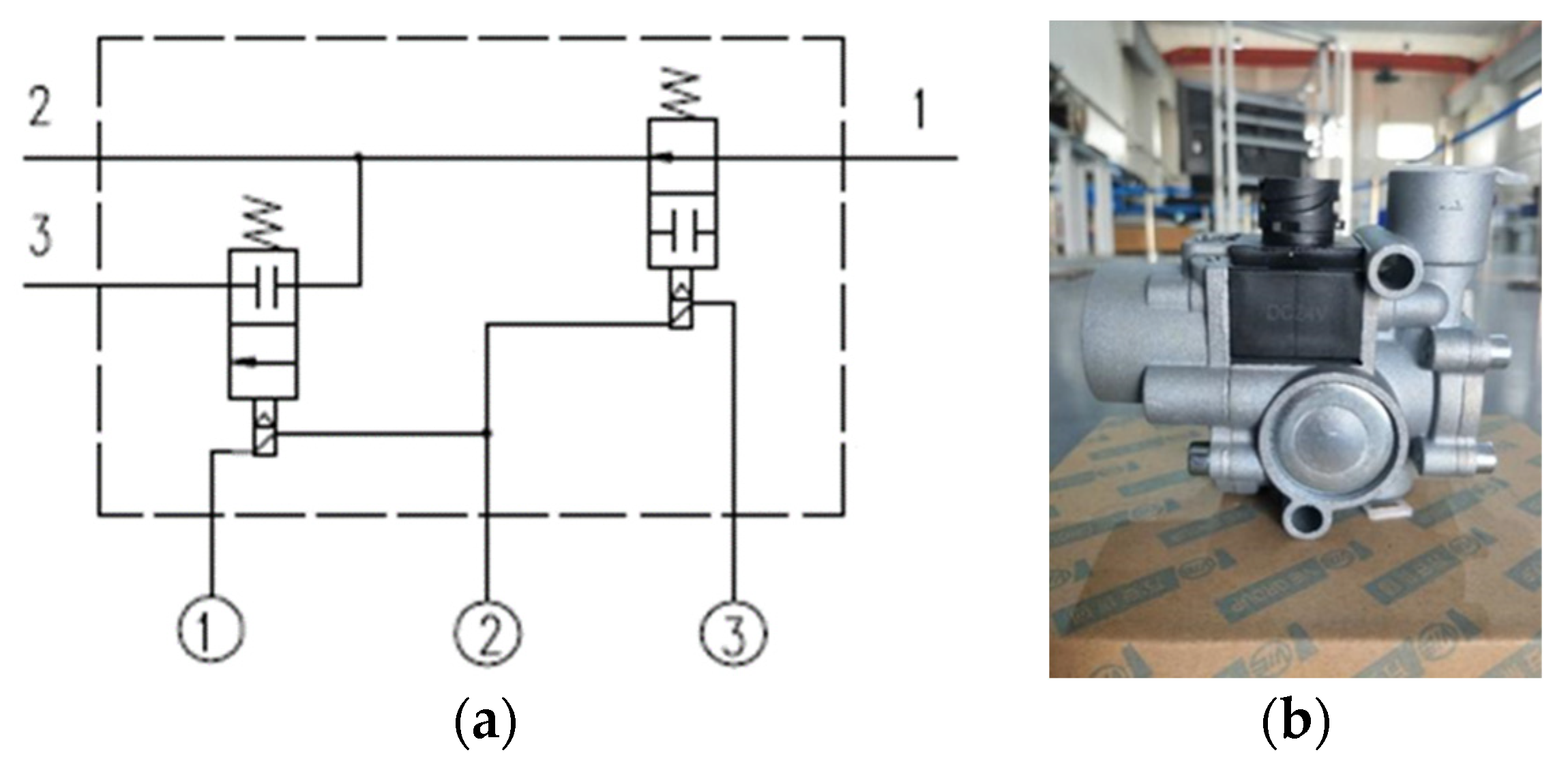
3.3. Working Principle and Modeling of ABS Electromagnetic Valve

The front axle uses a single-channel bridge control module and two ABS solenoid valves to control the pressure of the front-axle brake chamber. The ABS solenoid valve is mainly used to control the pressure of the brake chamber and is usually activated when the vehicle is in an emergency braking state. Through the precise regulation of the wheel brake chamber pressure, it becomes possible to effectively maintain the wheel slip rate in a desirable range. This proactive measure mitigates potential hazards such as lateral skidding or rotational instability resulting from complete wheel immobilization.

In Figure 13, the working principle diagram and physical diagram of the ABS solenoid valve are shown, respectively. When the driver brakes, the central ECU collects signals from the brake signal sensor and wheel speed sensor to determine whether it is in regular or emergency braking mode. When the vehicle is in regular braking mode, the ABS solenoid valve does not work, and the gas from the output port of the single-channel bridge control module can entirely enter the left and right brake chambers of the front axle for braking. During instances of emergency braking, the functioning of the ABS solenoid valve becomes pivotal. Operating in conjunction with the antilock braking algorithm, the valve undertakes crucial tasks such as pressurization, depressurization, and pressure regulation in the brake chamber.

As shown in Figure 13, the ABS solenoid valve consists of an intake valve and an exhaust valve, where port 1 is the air inlet, port 2 is the air outlets, and port 3 is the exhaust ports. ① + ② are the pressure-reducing coil. ② + ③ are the pressure-retaining coil.

When in a pressurized state, the intake valve is de-energized and the exhaust valve is de-energized. When in a reduced pressure state, the intake valve is energized and the exhaust valve is energized. When in a pressure-maintaining state, the intake valve is energized and the exhaust valve is de-energized. The working characteristics of the ABS solenoid valve are shown in

Table 3. Operating characteristics of ABS solenoid valve.

	Intake Valve	Exhaust Valve
Boosting	power outage	power outage
Reduce pressure	power on	power on
Maintaining pressure	power on	power outage

.

Utilizing the operational principles inherent in the ABS solenoid valve, a comprehensive model of the valve was constructed. The model, depicted in Figure 14, serves as an accurate representation of the ABS solenoid valve and its intricate functionality.

The response of output pressure with time is shown in Figure 15 for when the gas source pressure is 0.2 MPa and 0.4 MPa, respectively. By observing the figure, it is evident that the experimental data of the valve closely align with the simulated data, indicating that the model effectively captures the dynamic response of the valve under the specified operating condition.

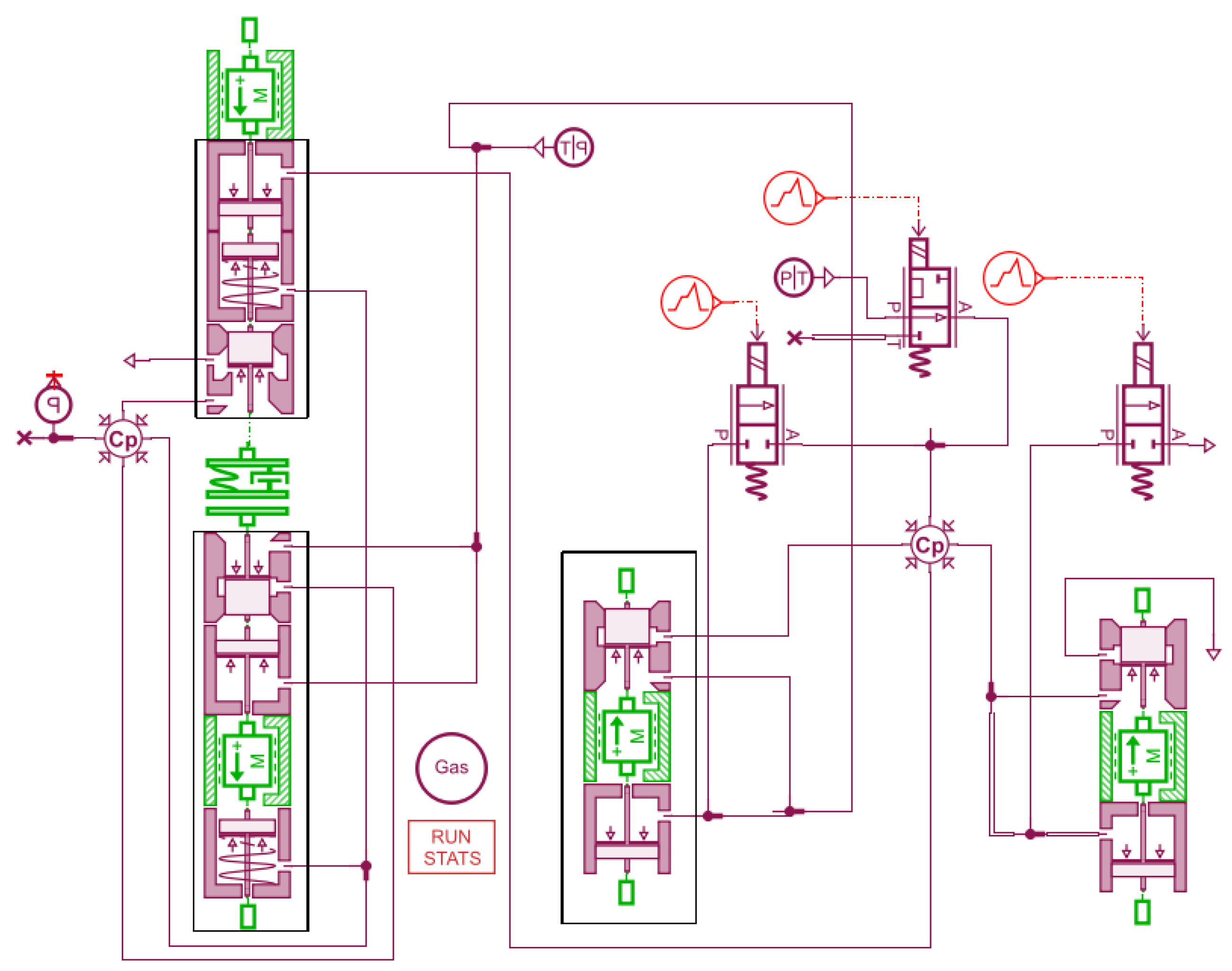
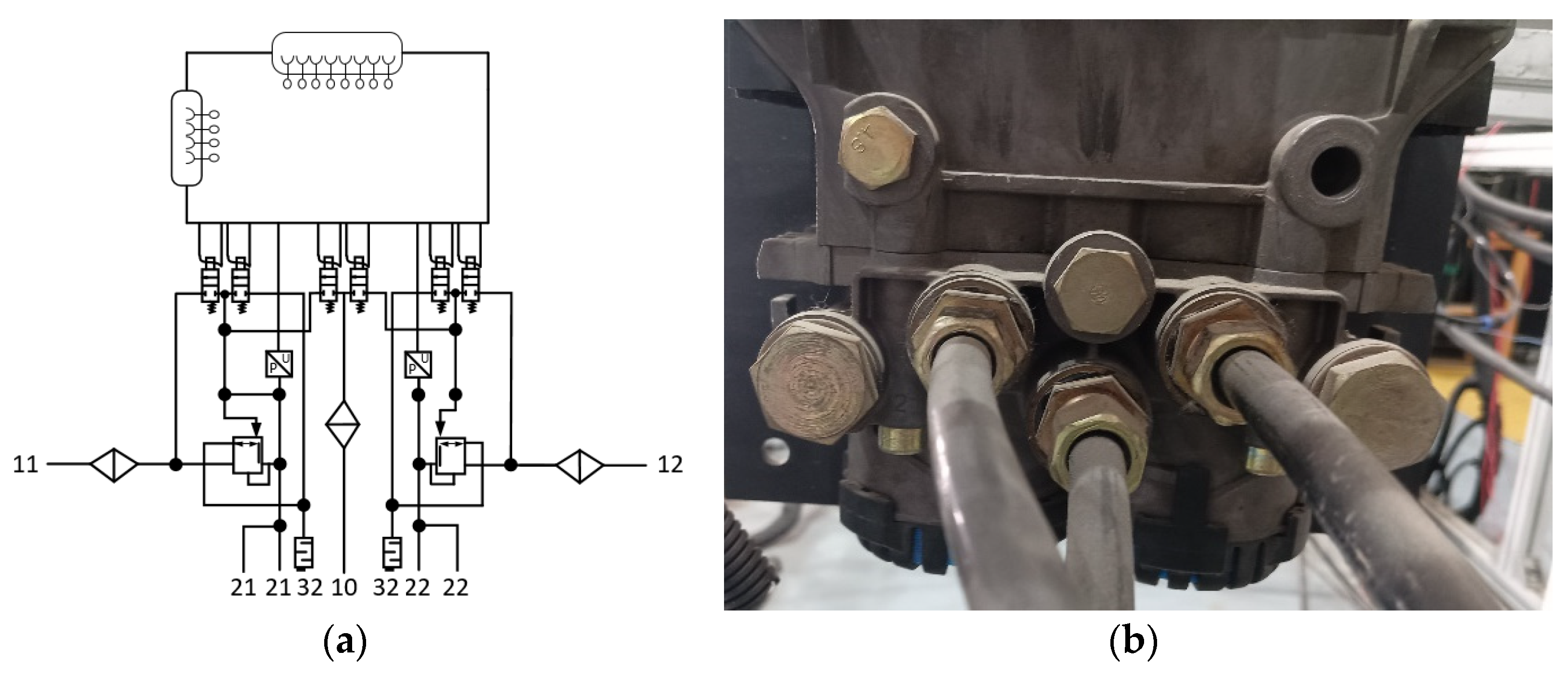
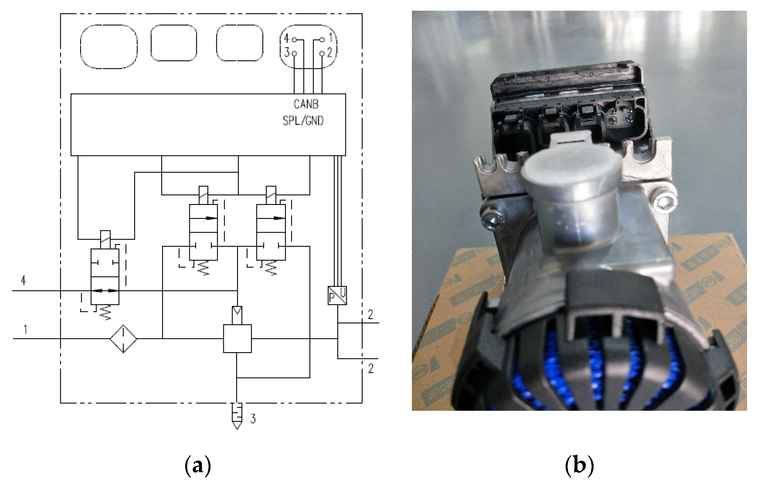
3.4. Working Principle and Modeling of Dual-Channel Bridge Control Module

For regulating the brake chamber pressure, a dual-channel bridge control module was implemented on the rear axle. This module allows for independent control over the brake chambers located on the left and right sides of the rear axle, ensuring that their operations remain unaffected by each other in terms of physical transmission. Therefore, the braking function can be achieved through the central ECU under conventional and emergency braking conditions.

Figure 16 shows the working principle and physical diagram of the dual-channel bridge control module, respectively. It can be seen that the dual-channel bridge control module is composed of two single-channel bridge control modules, which control the pressure of the brake chambers on the left and right sides of the rear axle, respectively. While the vehicle is in motion, the dual-channel bridge control module receives instructions from the central electronic control unit (ECU) to carry out various associated functionalities.

As shown in Figure 16, the dual-channel bridge control module consists of two sets of solenoid valves, each containing a boost solenoid valve, a pressure-reducing solenoid valve, and a backup solenoid valve. By coordinating the actions of two sets of solenoid valves, the pressure regulation of the brake chamber is achieved. In the pneumatic control circuit, ports 11 and 12 are air intakes, respectively, connected to the air storage cylinder. Ports 21 and 22 are air outlets, respectively, connected to the left and right brake chambers. Ports 31 and 32 are control ports, respectively, connected to the brake signal sensor. Port 4 corresponds to exhaust ports. When the electronic control circuit fails, the normal operation of the dual-channel bridge control module is ensured through pneumatic control.

The working characteristics of the dual-channel bridge control module in the electronic control circuit are shown in

Table 4. Operating characteristics of the left valve system of the dual-channel bridge control module.

	Boost Valve	Pressure-Reducing Valve	Backup Valve
Boosting	power on	power outage	power on
Reduce pressure	power outage	power on	power on
Maintaining pressure	power outage	power outage	power on

and

Table 5. Operating characteristics of the right valve system of the dual-channel bridge control module.

	Boost Valve	Pressure-Reducing Valve	Backup Valve
Boosting	power on	power outage	power on
Reduce pressure	power outage	power on	power on
Maintaining pressure	power outage	power outage	power on

.

Based on the working principle of the dual-channel bridge control module, a dual-channel bridge control module model was developed, as shown in Figure 17.

As illustrated in Figure 18, variation in the output pressure over time is observed when subjected to a gas source pressure of 0.2 MPa. From the figure, it can be seen that the experimental data of the valve are basically consistent with the simulation data, and the model can reflect the dynamic response of the valve under this working condition.

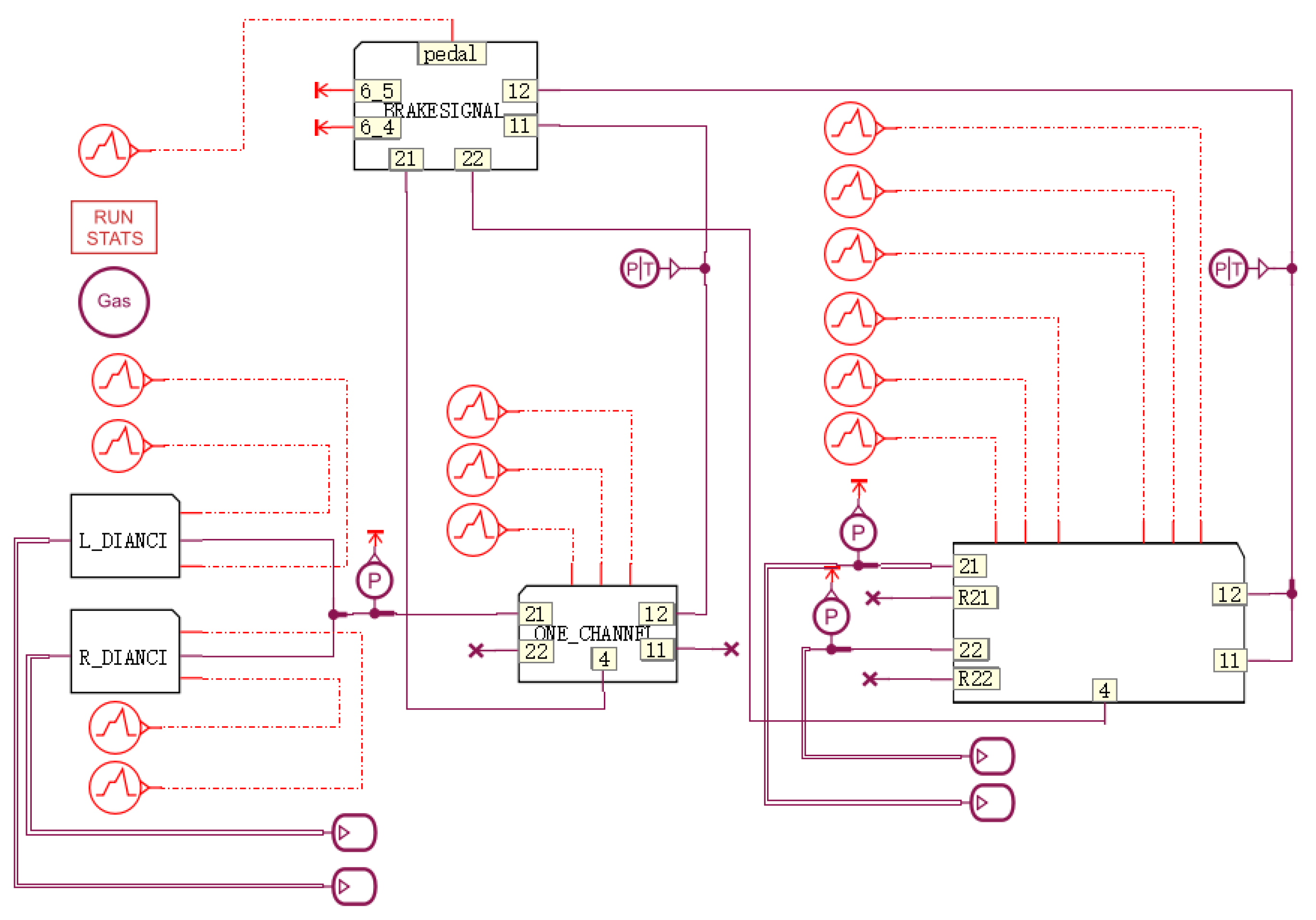
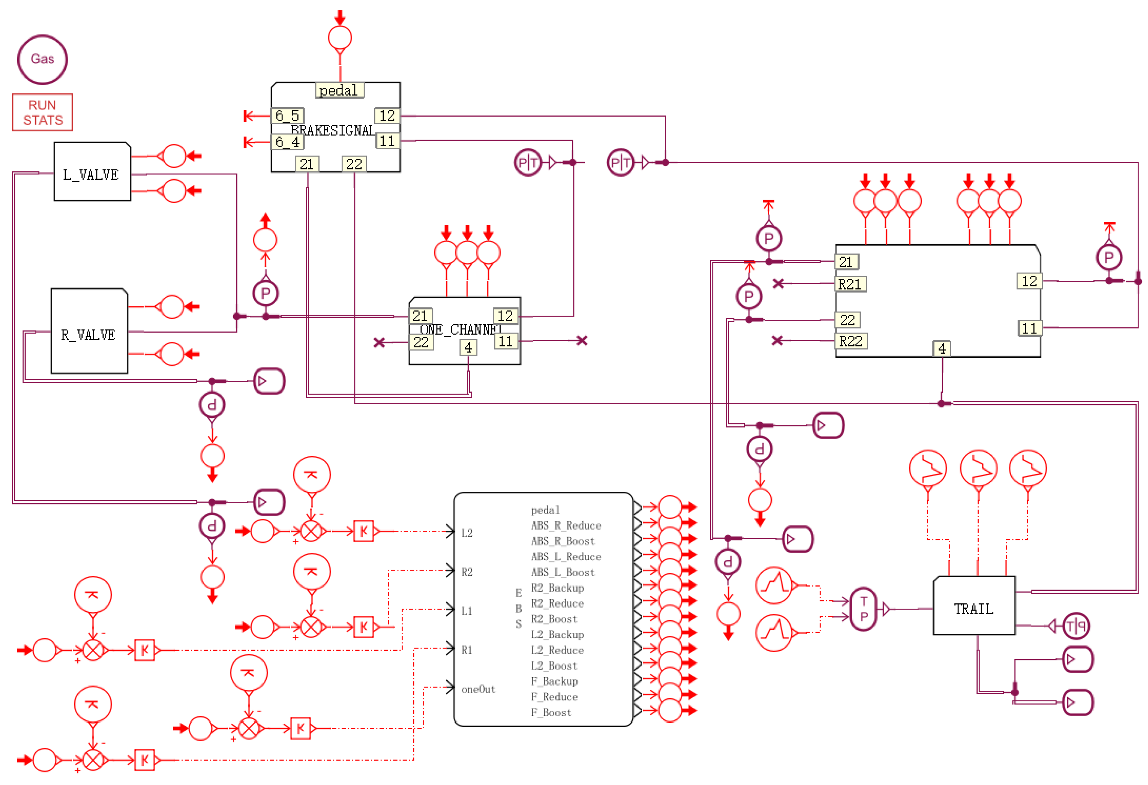
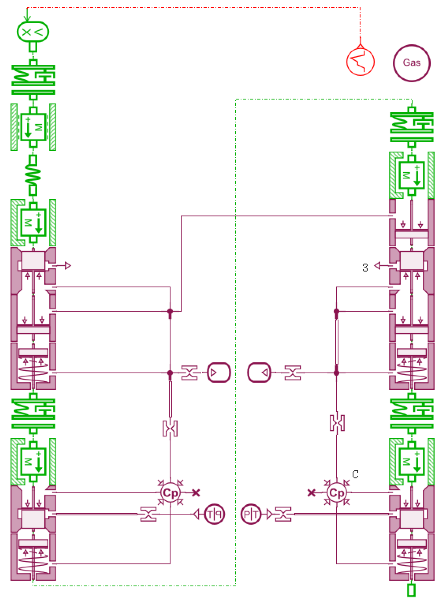
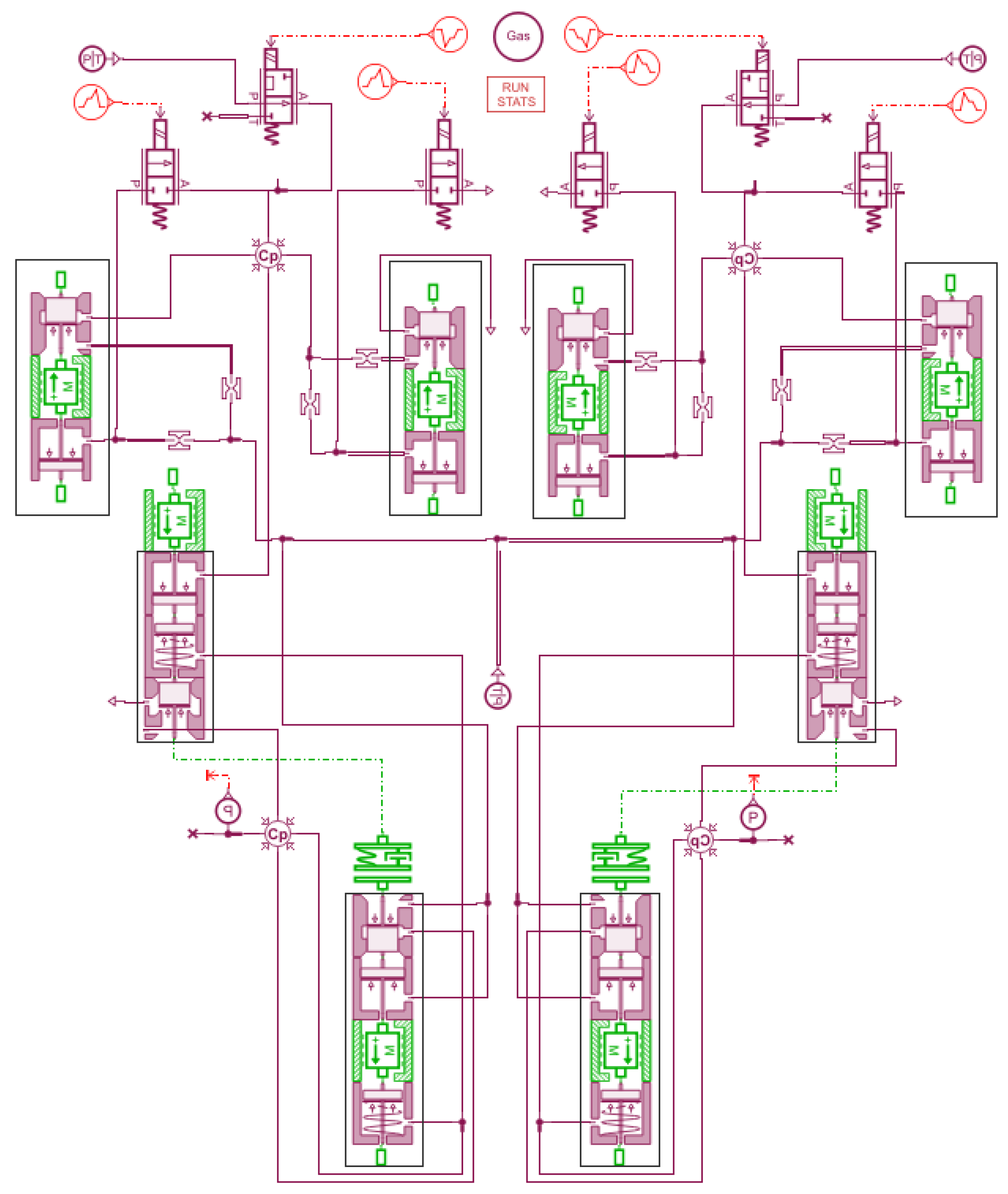
3.5. Dynamic Model of a Commercial Vehicle EBS

Based on the established models for the brake signal sensor, single-channel bridge control module, ABS solenoid valve, and dual-channel bridge control module, each module was encapsulated, ensuring their integration and functional compatibility, and models such as brake chambers and air pressure pipelines were established. Finally, an EBS dynamic model was established, as shown in Figure 19.

4. Design of a Commercial Vehicle EBS Control Algorithm

4.1. EBS Valve Control Algorithm

In a commercial vehicle EBS, the control of the valve is of great significance for the braking effect of the vehicle. In an EBS, the main power transmission medium is air, which has high compressibility and for which it is difficult to achieve precise control. Hence, upon calculating the desired braking force, it becomes imperative to rapidly and precisely regulate the valve to attain the intended pressure within the brake chamber.

During the regular braking process, the single-channel bridge control module and the dual-channel bridge control module are responsible for controlling the pressure in the brake chambers of the front- and rear-axle wheels of the vehicle. Given the analogous structure and operational principles of single- and dual-channel bridge control modules, this investigation primarily focused on examining the pressure regulation of single-channel bridge control modules.

The single-channel bridge control module mainly consists of a boost solenoid valve, a pressure-reducing solenoid valve, and a backup solenoid valve. Due to its complex structure, the motion process is difficult to describe and an accurate mathematical model cannot be established. Therefore, this study employed the pulse width modulation (PWM) signal method to enhance the precision of pressure regulation. By modulating the duty cycle, the valve’s outlet pressure was effectively adjusted. In order to accelerate the response time and avoid pressure overshoot during the control process as much as possible, this study adopted control algorithms based on threshold values for step boosting, step reducing, and pressure maintaining. When the actual pressure is much lower than the target pressure, rapid pressurization is required to accelerate the response time. When the actual pressure is lower than the target pressure, it is necessary to slowly pressurize to avoid overshoot and reduce oscillation. When the actual pressure is greater than the target pressure, it is necessary to slowly reduce the pressure to avoid overshoot and reduce oscillation. When the actual pressure is much greater than the target pressure, rapid decompression is needed to accelerate the response time. When the actual pressure is not significantly different from the target pressure, it is necessary to maintain the pressure. The precise computational procedures are presented in Equations (31)–(34).

(1)

When the actual pressure at the output port of the valve $P_a<P_{d2}$, the valve needs to be rapidly pressurized.

$$P_{d2}=P_t{s}_{d2}$$

(31)

$P_{d2}$ is the lower limit of the threshold value, and $s_{d2}$ is the proportional parameter obtained through empirical debugging.

(2)

When the actual pressure at the output port of the valve $P_a<P_{d1}$, the valve needs to be slowly pressurized.

$$P_{d1}=P_t{s}_{d1}$$

(32)

$P_{d1}$ is the lower limit of the threshold value, and $s_{d1}$ is the proportional parameter obtained through empirical debugging.

(3)

When the actual pressure at the output port of the valve $P_a>P_{u1}$, the valve needs to be slowly depressurized.

$$P_{u1}=P_t{s}_{u1}$$

(33)

$P_{u1}$ is the lower limit of the threshold value, and $s_{u1}$ is the proportional parameter obtained through empirical debugging.

(4)

When the actual pressure at the output port of the valve $P_a>P_{u2}$, the valve needs to be quickly depressurized.

$$P_{u2}=P_t{s}_{u2}$$

(34)

$P_{u2}$ is the lower limit of the threshold value, and $s_{u2}$ is the proportional parameter obtained through empirical debugging.

(5)

When the actual pressure at the output port of the valve is $P_{d1}<P_a<P_{u1}$, the valve needs to maintain pressure.

As illustrated in

Table 6. Valve duty cycle.

	Boost Valve	Pressure-Reducing Valve	Backup Valve
Quick boost	100%	0%	100%
Slow boost	50%	0%	100%
Maintain pressure	0%	0%	100%
Slowly reduce pressure	0%	50%	100%
Quickly reduce pressure	0%	100%	100%

, in accordance with the operational mechanism of the valve, during the accelerated boosting phase, the energization of the boost solenoid valve occurs, and the duty cycle is adjusted to 100%. The pressure-reducing solenoid valve is de-energized and the duty cycle is set to 0%. During the slow-boost phase, the boost solenoid valve is energized and the duty cycle is set to 50%. The pressure-reducing solenoid valve is de-energized and the duty cycle is set to 0%. During the slow-pressure-reduction phase, the boost solenoid valve is de-energized and the duty cycle is set to 0%. The relief solenoid valve is energized and the duty cycle is set to 100%. In the rapid-pressure-reduction stage, the boost solenoid valve is de-energized, the duty cycle is set to 0%, the pressure reduction solenoid valve is turned on, and the duty cycle is set to 100%. During the pressure maintenance stage, the boost solenoid valve and the pressure-reducing solenoid valve are deactivated, and the duty cycle is adjusted to 0%. In the above process, assuming that the electronic control system is normal, the backup solenoid valve is energized with a duty cycle of 100%.

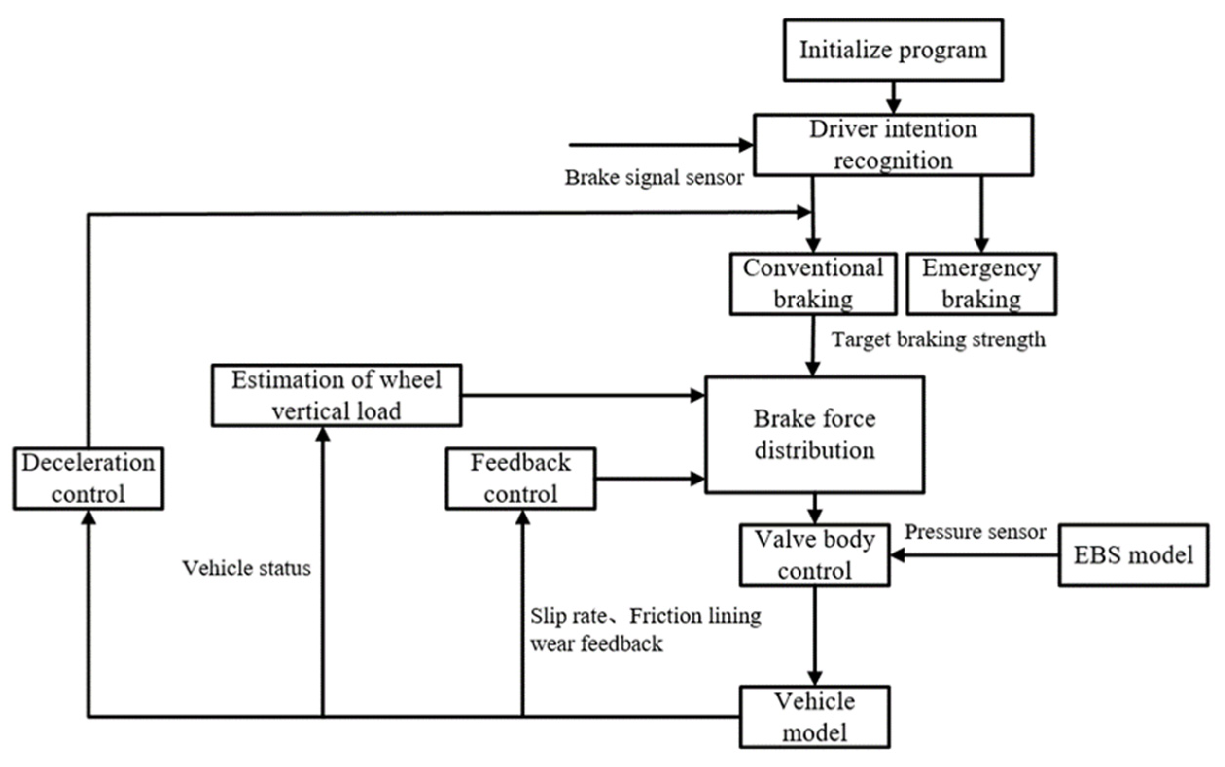
4.2. EBS Control Algorithm Process

This study mainly focuses on the research of commercial vehicle EBS control algorithms during the conventional braking process, including vertical load estimation, driver intention recognition, brake force distribution control, deceleration control, and valve control algorithms. The process is shown in Figure 20.

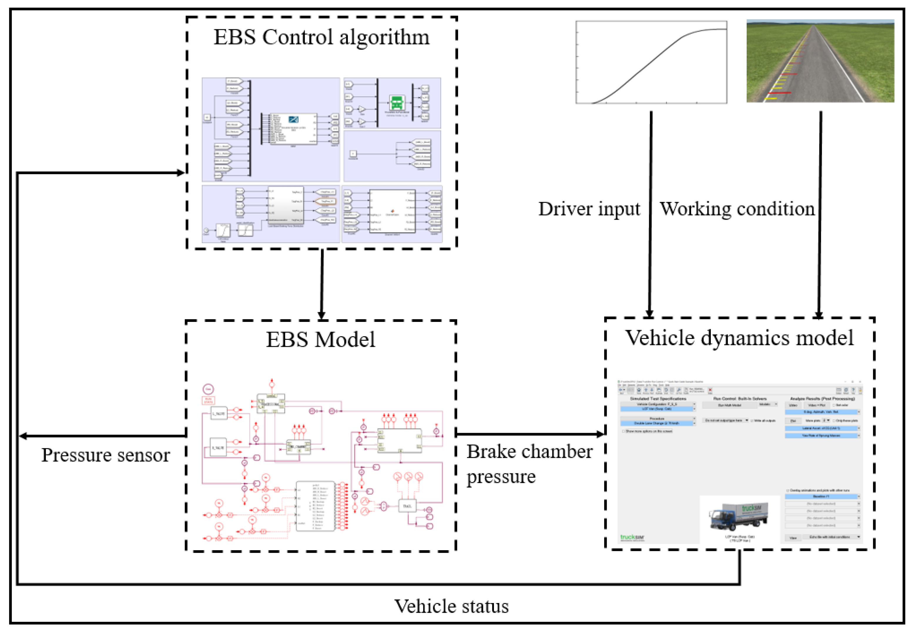
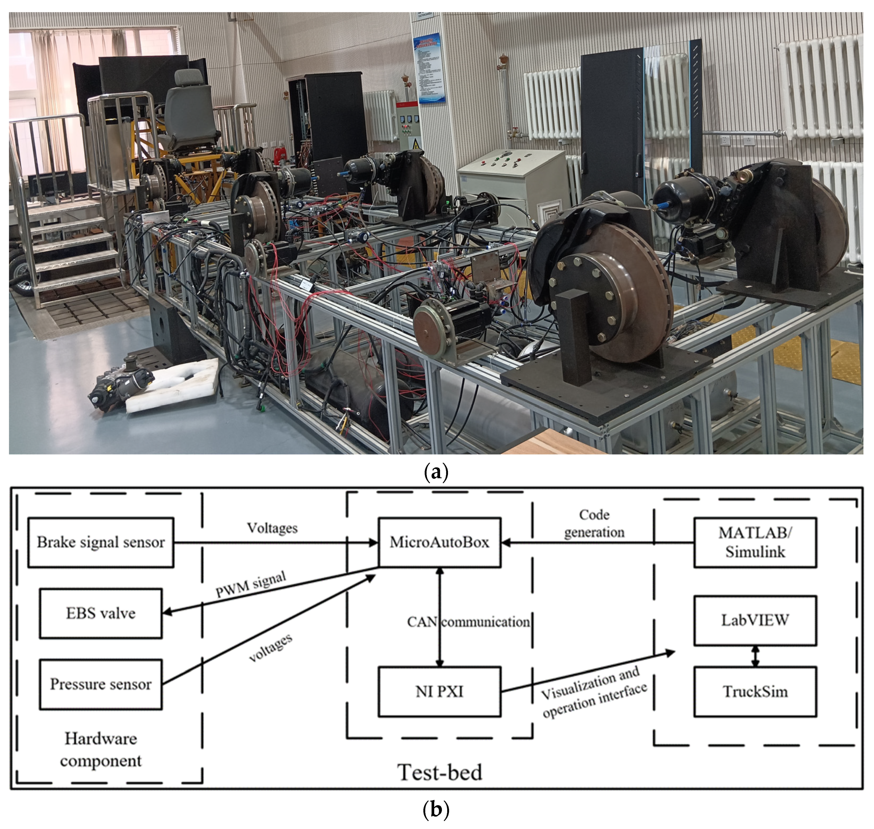
5. Hardware-in-the-Loop Experimental Verification of the Commercial Vehicle EBS Control Algorithm

In order to quickly and accurately develop the EBS control algorithm and facilitate debugging, this study established a commercial vehicle EBS control algorithm simulation platform. The platform primarily encompasses the following components: a vehicle dynamics model, an electronic braking system (EBS) model, and an EBS valve control algorithm. The overall architecture of the platform is shown in Figure 21.

In terms of interface settings, the EBS dynamics model mainly receives the target pressure from the EBS valve control algorithm and outputs the actual pressure to the vehicle dynamics model. Figure 22 showcases the interface configurations for the dynamic model of the electronic braking system (EBS) and the collaborative simulation.

The simulation platform developed in this research for cohesive joint simulation purposes. The overall architecture of the EBS hardware-in-the-loop experimental platform built in this study is shown in Figure 23.

In order to verify the developed EBS control algorithm, based on the hardware-in-the-loop experimental platform built, this study used various operating conditions for verification, including brake force distribution control and deceleration control.

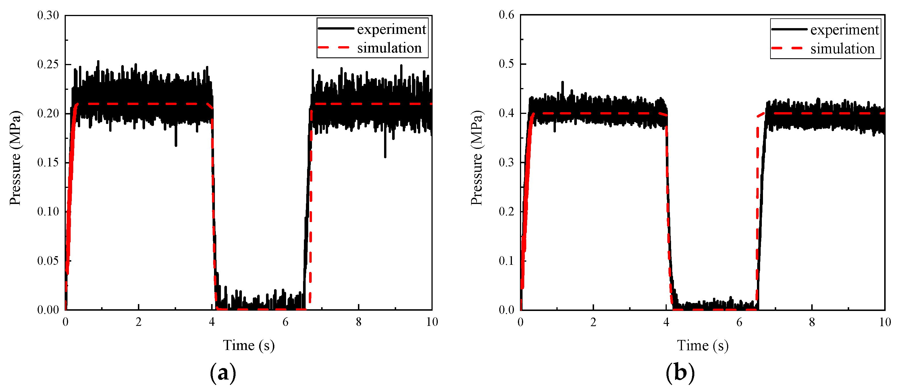
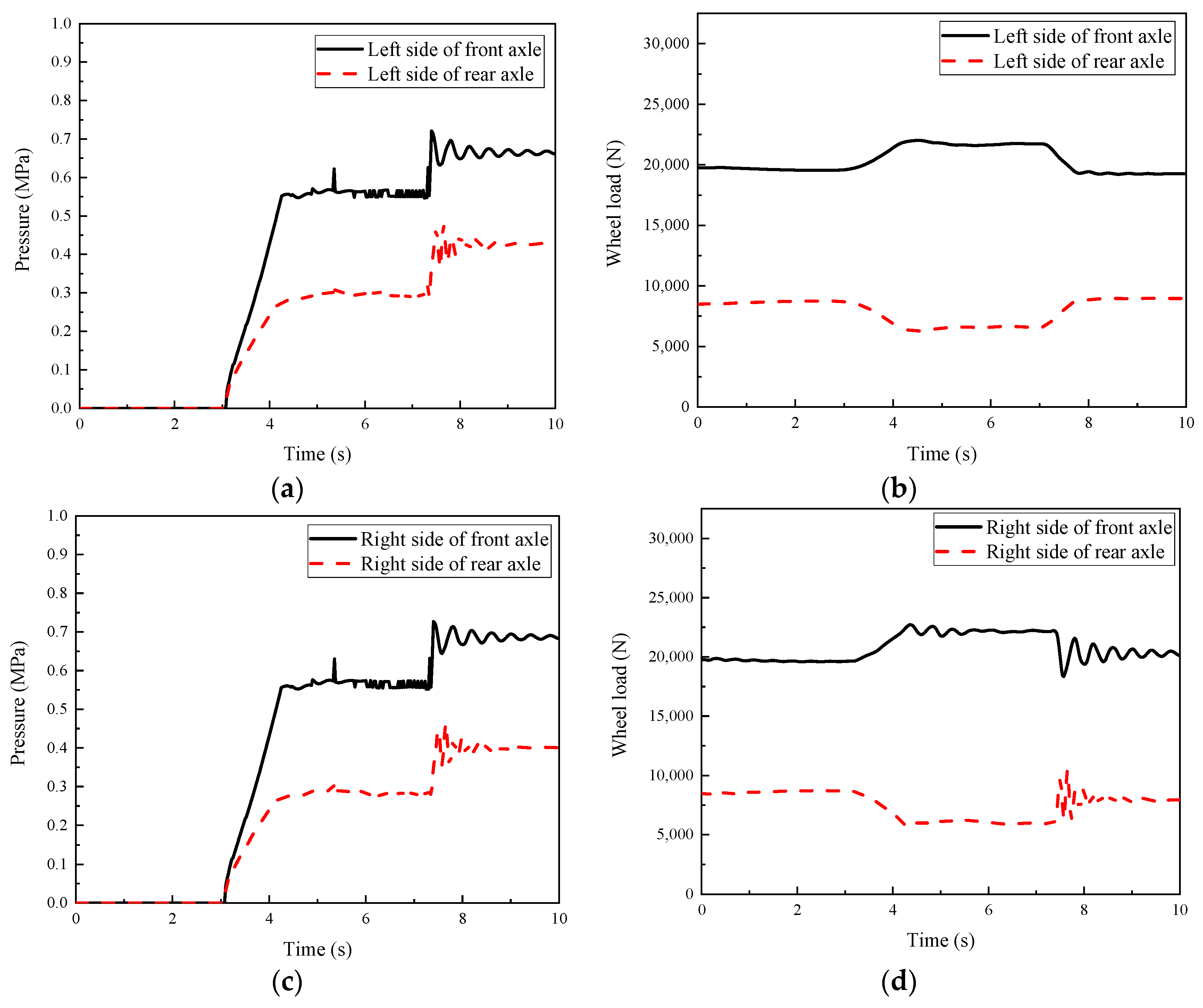
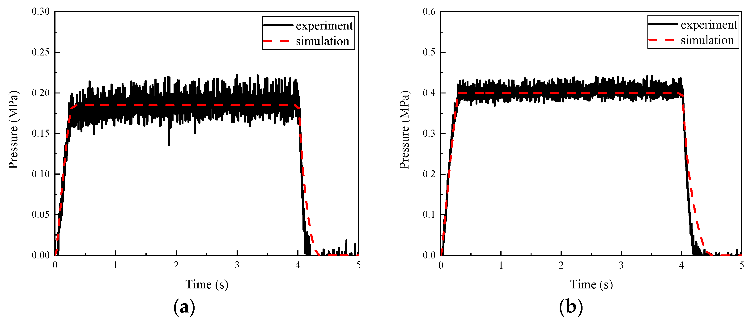
5.1. Experimental Verification of Brake Force Distribution Control

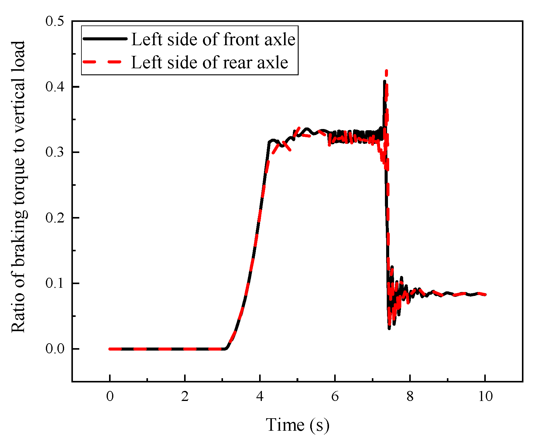
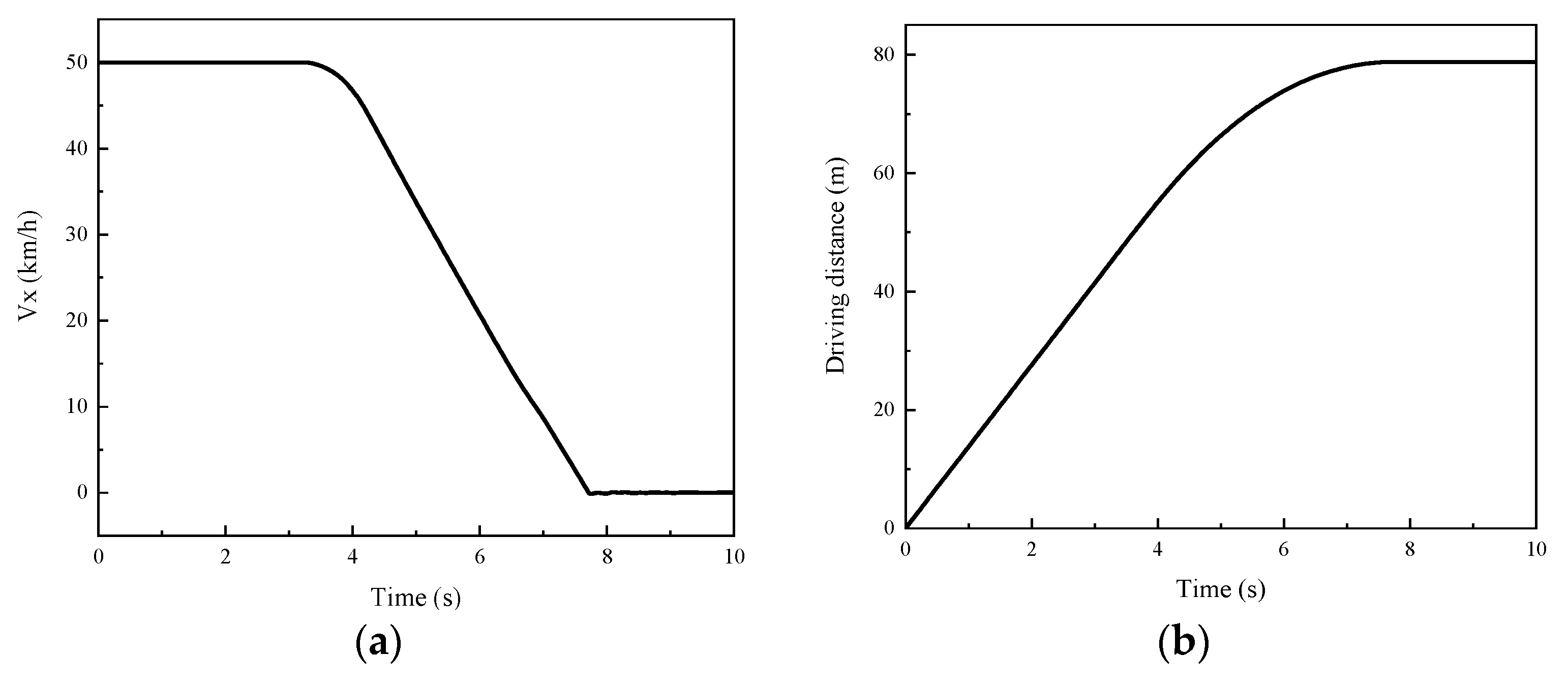
5.1.1. Unloaded Condition

When the vehicle was operating without any load, starting at an initial velocity of 50 km/h and an adhesion coefficient of 0.85, the throttle aperture gradually transitioned from 0% to 50%. The test results are shown in Figure 24, Figure 25 and Figure 26. As shown in Figure 24, in the initial stage, the speed could not be kept constant. At 3 s, the vehicle began to brake, and there was a certain delay in establishing pressure in the wheel brake chamber. At 7.3 s, the vehicle speed decreased to 0. Due to the fact that the target braking strength is only related to the pedal opening and the pedal had not yet been released, the difference between the target braking strength and the actual braking strength was too large. Therefore, the brake pressure of the front and rear wheels continued to increase, and its maximum value was related to the vertical load of the wheels. As depicted in Figure 25, following the initiation of braking, the displacement of the vehicle’s center of mass resulted in an augmentation of the front-axle load while concurrently diminishing the rear-axle load. After the vehicle speed decreased to 0, the front- and rear-axle loads of the vehicle returned to the state before braking. As shown in Figure 26, the ratio of the braking torque of the front- and rear-axle wheels of the vehicle to the vertical load was equal, indicating that the braking torque of the front and rear wheels of the vehicle dynamically changed with the vertical load.

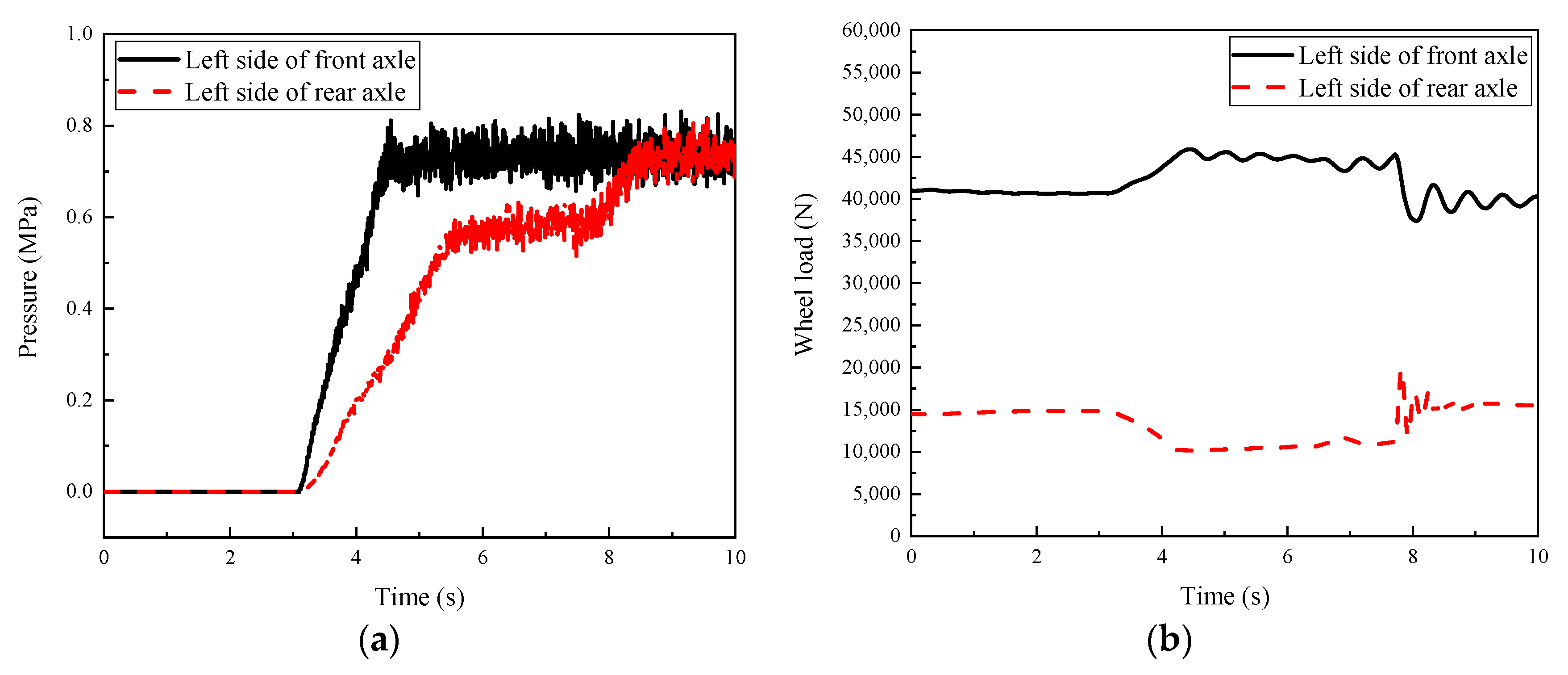
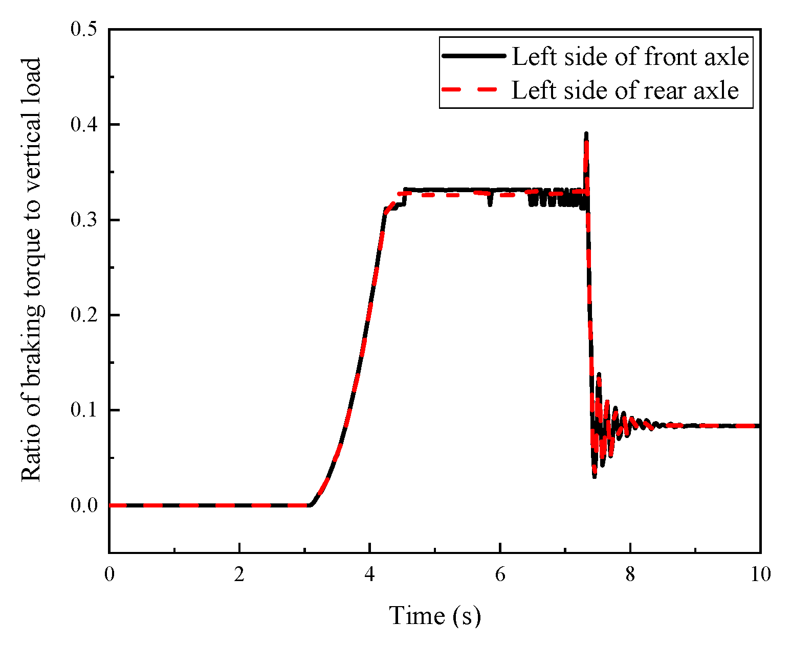
5.1.2. Full-Load Condition

In the scenario where the vehicle was under maximum load capacity, commencing at an initial velocity of 50 km/h and an adhesion coefficient of 0.85, the throttle aperture steadily transitioned from 0% to 50%. The test results are shown in Figure 27, Figure 28 and Figure 29. As shown in Figure 27, at 3 s, the vehicle began to brake, and there was a certain delay in establishing pressure in the wheel brake chamber. At 7.4 s, the vehicle speed decreased to 0. Although there was a significant difference between the target braking strength and the actual braking strength at this time, due to the large vertical load on the wheels, the front wheel braking pressure reached its maximum, and the rear wheel braking pressure continued to increase and reach its maximum. As shown in Figure 28, after the vehicle braked, due to the forward movement of the center of mass, the front-axle load of the vehicle increased and the rear-axle load decreased. After the vehicle speed decreased to 0, the front- and rear-axle loads of the vehicle returned to the state before braking. As shown in Figure 29, the ratio of the braking torque of the front- and rear-axle wheels of the vehicle to the vertical load was equal, indicating that the braking torque of the front and rear wheels of the vehicle dynamically changed with the vertical load.

Based on the experimental verification and analysis conducted above, the braking force distribution control algorithm mentioned in this study can effectively utilize ground adhesion conditions and achieve good braking effects.

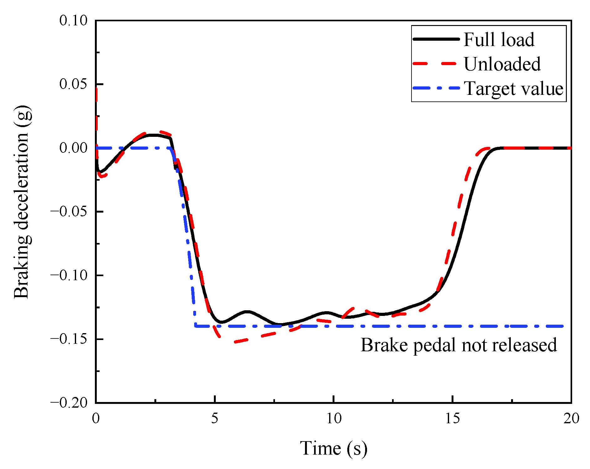
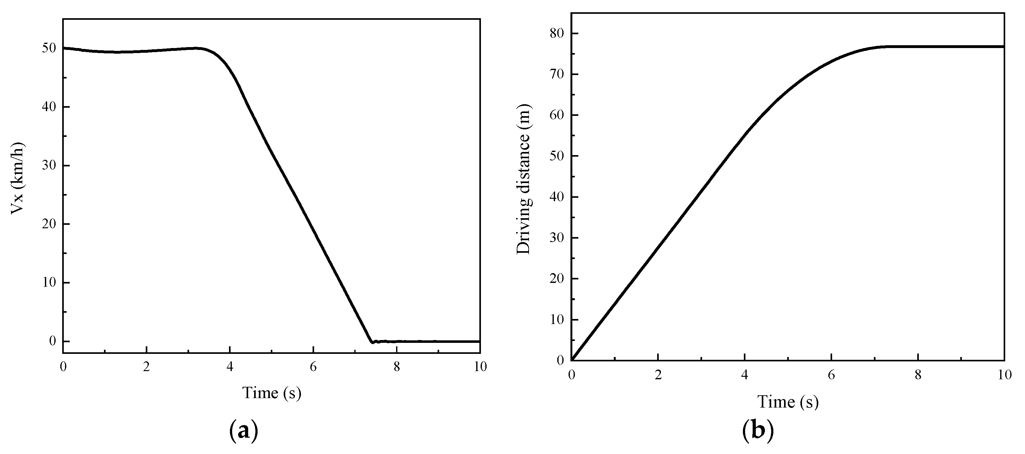
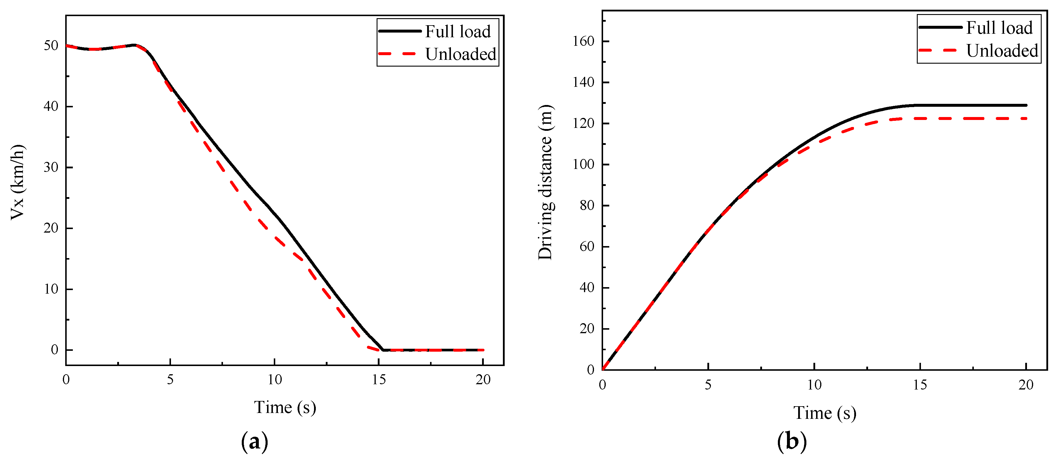
5.2. Experimental Verification of Deceleration Control

5.2.1. Pedal Stroke 30%

When the vehicle was fully loaded and unloaded, with an initial speed of 50 km/h and an adhesion coefficient of 0.85, the pedal opening gradually changed from 0 to 30%. The test results are shown in Figure 30 and Figure 31. As shown in Figure 30, in the initial stage, the speed could not be kept constant. The vehicle started braking at 3 s, and the braking deceleration of the vehicle was basically equal to the target braking deceleration. At 15 s, the vehicle speed decreased to 0. At this point, the pedal had not yet been released, so the target braking deceleration remained unchanged, but the actual braking deceleration became 0. The simulation findings indicate that when the throttle aperture reached 30%, the vehicle demonstrated consistent braking deceleration across varying loads.

5.2.2. Pedal Stroke 50%

When the vehicle was fully loaded and unloaded, with an initial speed of 50 km/h and an adhesion coefficient of 0.85, the pedal opening gradually changed from 0 to 50%. The test results are shown in Figure 32 and Figure 33. As shown in Figure 32, the vehicle started braking at 3 s, and the braking deceleration of the vehicle was basically equal to the target braking deceleration. At 7.3 s, the vehicle speed decreased to 0. At this point, the pedal had not yet been released, so the target braking deceleration remained unchanged, but the actual braking deceleration became 0. The simulation results demonstrate that at a throttle aperture of 50%, the vehicle exhibited uniform braking deceleration across diverse load conditions.

Based on the experimental verification and analysis conducted above, the deceleration control algorithm mentioned in this study can generate the same deceleration for vehicles under different loads and the same pedal opening, verifying the effectiveness of the algorithm.

6. Conclusions

This study focused on the characteristics and control algorithms of a commercial vehicle EBS. Based on the analysis of existing research content at home and abroad, the following work was carried out:

(1)

A commercial vehicle EBS dynamic model was established, including a brake signal sensor, a single-channel bridge control module, an ABS solenoid valve, and a dual-channel bridge control module.

(2)

A vertical load estimation algorithm based on UPF was designed, enabling the real-time estimation of wheel vertical load during vehicle operation.

(3)

This study developed an algorithm based on the characteristics of the EBS valve in order to quickly and accurately control the valve. And based on a hardware-in-the-loop experimental platform, the above algorithm was analyzed to verify the effectiveness of the control algorithm.

References

1. Zhao, J.; Wu, X.; Song, Z.; Sun, L.; Wang, X. Practical hybrid model predictive control for electric pneumatic braking system with on-off solenoid valves. Proc. Inst. Mech. Eng. Part D J. Automob. Eng. 2023. [Google Scholar] [CrossRef]
2. Zhao, Y.; Yang, Y.; Wu, X.; Tao, X. Research on accurate modeling and control for pneumatic electric braking system of commercial vehicle based on multi-dynamic parameters measurement. Proc. Inst. Mech. Eng. Part D J. Automob. Eng. 2023, 237, 803–815. [Google Scholar] [CrossRef]
3. Hamada, A.T.; Orhan, M.F. An overview of regenerative braking systems. J. Energy Storage 2022, 52, 105033. [Google Scholar] [CrossRef]
4. Shan, T.; Li, L.; Wu, X.; Cheng, S. Pressure control based on reinforcement learning strategy of the pneumatic relays for an elec-tric-pneumatic braking system. Proc. Inst. Mech. Eng. Part D J. Automob. Eng. 2022, 237, 09544070221108855. [Google Scholar]
5. Zhang, L.; Yan, Y.; Zhu, Q.; Zhao, G.; Feng, D.; Wu, J. A Pneumatic Control Method for Commercial Vehicle Electronic Brake System Based on EPV Module. Actuators 2022, 11, 316. [Google Scholar] [CrossRef]
6. Wu, J.; Kong, Q.; Yang, K.; Liu, Y.; Cao, D.; Li, Z. Research on the steering torque control for intelligent vehicles co-driving with the penalty factor of human–machine intervention. IEEE Trans. Syst. Man Cybern. Syst. 2022, 53, 59–70. [Google Scholar] [CrossRef]
7. Yan, Y.; Wu, J.; Liu, X.; Zhao, Y.; Wang, S. A lateral trajectory tracking control method for intelligent commercial vehicles considering active anti-roll decision based on Stackelberg equilibrium. IET Intell. Transp. Syst. 2022, 16, 1193–1208. [Google Scholar] [CrossRef]
8. Li, G.; Wei, X.; Wang, Z.; Bao, H. Study on the Pressure Regulation Method of New Automatic Pressure Regulating Valve in the Electronically Controlled Pneumatic Brake Systems in Commercial Vehicles. Sensors 2022, 22, 4599. [Google Scholar] [CrossRef]
9. Zhang, R.; Peng, J.; Li, H.; Chen, B.; Liu, W.; Huang, Z.; Wang, J. A predictive control method to improve pressure tracking precision and reduce valve switching for pneumatic brake systems. IET Control. Theory Appl. 2021, 15, 1389–1403. [Google Scholar] [CrossRef]
10. Zhao, Q.; Zheng, H.; Kaku, C.; Cheng, F.; Zong, C. Safety spacing control of truck platoon based on emergency braking under different road conditions. SAE Int. J. Veh. Dyn. Stab. NVH 2022, 7, 69–81. [Google Scholar] [CrossRef]
11. Bao, H.; Wang, Z.; Liu, Z.; Li, G. Study on Pressure Change Rate of the Automatic Pressure Regulating Valve in the Electronic-Controlled Pneumatic Braking System of Commercial Vehicle. Processes 2021, 9, 938. [Google Scholar] [CrossRef]
12. Zhao, Y.; Yang, Y. Pressure control for pneumatic electric braking system of commercial vehicle based on model predictive control. IET Intell. Transp. Syst. 2021, 15, 1522–1532. [Google Scholar] [CrossRef]
13. Wu, X.; Li, L.; Wang, X.; Chen, X.; Cheng, S. Nonlinear controller design and testing for chatter suppression in an electric-pneumatic braking system with parametric variation. Mech. Syst. Signal Process. 2020, 135, 106401. [Google Scholar] [CrossRef]
14. Yang, Y.; Tang, Q.; Bolin, L.; Fu, C. Dynamic coordinated control for regenerative braking system and anti-lock braking system for electrified vehicles under emergency braking conditions. IEEE Access 2020, 8, 172664–172677. [Google Scholar] [CrossRef]
15. Leng, B.; Xiong, L.; Yu, Z.; Sun, K.; Liu, M. Robust variable structure anti-slip control method of a distributed drive electric vehicle. IEEE Access 2020, 8, 162196–162208. [Google Scholar] [CrossRef]
16. Han, W.; Xiong, L.; Yu, Z. Interconnected pressure estimation and double closed-loop cascade control for an integrated electro-hydraulic brake system. IEEE/ASME Trans. Mechatron. 2020, 25, 2460–2471. [Google Scholar] [CrossRef]
17. Xu, C.; Zhao, W.; Li, L.; Chen, Q.; Kuang, D.; Zhou, J. A nash Q-learning based motion decision algorithm with considering interaction to traffic partici-pants. IEEE Trans. Veh. Technol. 2020, 69, 12621–12634. [Google Scholar] [CrossRef]
18. Zheng, H.; Ma, S.; Fang, L.; Zhao, W.; Zhu, T. Braking intention recognition algorithm based on electronic braking system in commercial ve-hicles. Int. J. Heavy Veh. Syst. 2019, 26, 268–290. [Google Scholar] [CrossRef]
19. Mishra, P.; Kumar, V.; Rana, K. An online tuned novel nonlinear PI controller for stiction compensation in pneumatic control valves. ISA Trans. 2015, 58, 434–445. [Google Scholar] [CrossRef]
20. Meng, F.; Zhang, H.; Cao, D.; Chen, H. System modeling, coupling analysis, and experimental validation of a proportional pressure valve with pulsewidth modulation control. IEEE/ASME Trans. Mechatron. 2015, 21, 1742–1753. [Google Scholar] [CrossRef]
21. Guo, J.; Li, W.; Wang, J.; Luo, Y.; Li, K. Safe and energy-efficient car-following control strategy for intelligent electric vehicles considering regenerative braking. IEEE Trans. Intell. Transp. Syst. 2021, 23, 7070–7081. [Google Scholar] [CrossRef]
22. Santini, S.; Albarella, N.; Arricale, V.M.; Brancati, R.; Sakhnevych, A. On-board road friction estimation technique for autonomous driving vehi-cle-following maneuvers. Appl. Sci. 2021, 11, 2197. [Google Scholar] [CrossRef]
23. Hellgren, J.; Jonasson, E. Maximisation of brake energy regeneration in a hybrid electric parallel car. Int. J. Electr. Hybrid Veh. 2007, 1, 95. [Google Scholar] [CrossRef]
24. Mosconi, L.; Farroni, F.; Sakhnevych, A.; Timpone, F.; Gerbino, F.S. Adaptive vehicle dynamics state estimator for onboard automotive applications and performance analysis. Veh. Syst. Dyn. 2022, 1–25. [Google Scholar] [CrossRef]
25. Chu, W.; Luo, Y.; Dai, Y.; Li, K. In–wheel motor electric vehicle state estimation by using unscented particle filter. Int. J. Veh. Des. 2015, 67, 115–136. [Google Scholar] [CrossRef]
26. Wang, Q.; Zhao, Y.; Xie, W.; Zhao, Q.; Lin, F. Hierarchical estimation of vehicle state and tire forces for distributed in-wheel motor drive electric vehicle without previously established tire model. J. Frankl. Inst. 2022, 359, 7051–7068. [Google Scholar] [CrossRef]
27. Lui, D.G.; Tartaglione, G.; Conti, F.; De Tommasi, G.; Santini, S. Long Short-Term Memory-Based Neural Networks for Missile Maneuvers Trajectories Prediction. IEEE Access 2023, 11, 30819–30831. [Google Scholar] [CrossRef]
28. Zhang, Y.; Li, M.; Zhang, Y.; Hu, Z.; Sun, Q.; Lu, B. An enhanced adaptive unscented kalman filter for vehicle state estimation. IEEE Trans. Instrum. Meas. 2022, 71, 6502412. [Google Scholar] [CrossRef]
29. Liu, H.; Wang, P.; Lin, J.; Ding, H.; Chen, H.; Xu, F. Real-time longitudinal and lateral state estimation of preceding vehicle based on moving horizon estimation. IEEE Trans. Veh. Technol. 2021, 70, 8755–8768. [Google Scholar] [CrossRef]
Figure 1. Vehicle dynamics model.
Actuators 12 00376 g001
Figure 2. Longitudinal force diagram of the vehicle.
Actuators 12 00376 g002
Figure 3. (a) Vertical load of left front-axle wheel; (b) vertical load of right front-axle wheel.
Actuators 12 00376 g003
Figure 4. (a) Vertical load of left rear-axle wheel; (b) vertical load of right rear-axle wheel.
Actuators 12 00376 g004
Figure 5. (a) Vertical load of left front-axle wheel; (b) vertical load of right front-axle wheel.
Actuators 12 00376 g005
Figure 6. (a) Vertical load of left rear-axle wheel; (b) load of right rear-axle wheel.
Actuators 12 00376 g006
Figure 7. (a) Working principle diagram of brake signal sensor, Port 1 and Port 2 are power supply ports, Port 3 is the exhaust port, Port 4 is a positive slope voltage output port, Port 5 is a negative slope voltage output port, Port 6 is the step signal output port, Ports 11 and 12 are air intakes, Port 21 and port 22 are exhaust ports; (b) physical diagram of brake signal sensor.
Actuators 12 00376 g007
Figure 8. Model of brake signal sensor. Port 3 is the exhaust port, Component C is the brake chamber, Green represents mechanical components, Light purple represents pneumatic components.
Actuators 12 00376 g008
Figure 9. (a) Port 21 pressure; (b) port 22 pressure.
Actuators 12 00376 g009
Figure 10. (a) Working principle diagram of single-channel bridge control module, Port 1 is the air inlet, Port 2 is the air outlet, Port 3 is the exhaust port, Port 4 is the control port, Pin 1 is the control wire of the pressure reducing solenoid valve, Pin 2 is the ground wire, Pin 3 is the control wire for the backup solenoid valve, Pin 4 is the control wire of the boost solenoid valve; (b) physical diagram of a single-channel bridge control module.
Actuators 12 00376 g010
Figure 11. Model of single-channel bridge control module. The red “x” represents a plug, Green represents mechanical components, Light purple represents pneumatic components.
Actuators 12 00376 g011
Figure 12. (a) Output pressure (0.2 MPa); (b) output pressure (0.4 MPa).
Actuators 12 00376 g012
Figure 13. (a) Working principle diagram of ABS solenoid valve, Port 1 is the air inlet, Port 2 is the air outlet, Port 3 is the exhaust port, ② + ③ is the pressure retaining coil, ② + ① is the pressure reducing coil; (b) physical image of ABS solenoid valve.
Actuators 12 00376 g013
Figure 14. Model of ABS solenoid valve. Green represents mechanical components, Light purple represents pneumatic components, The “x” represents a plug.
Actuators 12 00376 g014
Figure 15. (a) Output pressure (0.2 MPa); (b) output pressure (0.4 MPa).
Actuators 12 00376 g015
Figure 16. (a) Working principle diagram of dual-channel bridge control module, Port 10 is the exhaust port, Ports 11 and 12 are air intakes, Ports 21 and 22 are air outlets, Port 31 and 32 are control ports; (b) physical diagram of dual-channel bridge control module.
Actuators 12 00376 g016
Figure 17. Model of dual-channel bridge control module. Green represents mechanical components, Light purple represents pneumatic components, The “x” represents a plug.
Actuators 12 00376 g017
Figure 18. (a) Left output pressure (0.2 MPa); (b) right output pressure (0.2 MPa).
Actuators 12 00376 g018
Figure 19. EBS model. Ports 11 and 12 are air intakes, Ports 21 and 22 are air outlets, Port 4 is a communication port, Ports R21, R22, 6_ 4 and 6_ 5 is the exhaust port, Port pedal is the brake pedal, Light purple represents pneumatic components, Red represents electrical components, The “x” represents a plug.
Actuators 12 00376 g019
Figure 20. EBS control algorithm flowchart.
Actuators 12 00376 g020
Figure 21. EBS control algorithm simulation platform. The red and yellow in the road represent gaps. The red below represents electrical components.
Actuators 12 00376 g021
Figure 22. EBS dynamic model and interface settings. Light purple represents pneumatic components, Red represents electrical components, Ports 11 and 12 are air intakes, Ports 21 and 22 are air outlets, Port 4 is a communication port, Ports R21, R22, 6_ 4 and 6_ 5 is the exhaust port, Port pedal is the brake pedal, Port L1 represents the left side of the first axis, Port R1 represents the right side of the first shaft, Port L2 represents the left side of the second axis, Port R2 represents the right side of the second axis, Port oneOut represents the output port, Port ABS_ R_ Reduce represents the pressure reduction of the right ABS valve, Port ABS_ R_ Boost represents the right ABS valve boost, Port ABS_ L_ Reduce represents the pressure reduction of the left ABS valve, Port ABS_ L_ Boost represents the left ABS valve boost, Port R2_ Backup represents the backup valve on the right side of the second shaft, Port R2_ Reduce represents the pressure reducing valve on the right side of the second shaft, Port R2_ Boost represents the boost valve on the right side of the second shaft, Port L2_ Backup represents the backup valve on the left side of the second shaft, Port L2_ Reduce represents the pressure reducing valve on the left side of the second shaft, Port L2_ Boost represents the left boost valve of the second shaft, Port F_ Backup represents the front axle backup valve, Port F_ Reduce represents the front axle pressure reducing valve, Port F_ Boost represents the front axle boost valve, The “x” represents a plug.
Actuators 12 00376 g022
Figure 23. (a) The physical image of the hardware in the loop test bench; (b) Overall architecture of EBS hardware-in-the-loop experimental platform.
Actuators 12 00376 g023
Figure 24. (a) Vehicle speed; (b) driving distance.
Actuators 12 00376 g024
Figure 25. (a) Left-brake-chamber pressure of front and rear axles; (b) vertical load of left wheel on front and rear axles; (c) right-brake-chamber pressure of front and rear axles; (d) vertical load of right wheel on front and rear axles.
Actuators 12 00376 g025
Figure 26. Ratio of braking torque to vertical load.
Actuators 12 00376 g026
Figure 27. (a) Vehicle speed; (b) driving distance.
Actuators 12 00376 g027
Figure 28. (a) Left-brake-chamber pressure of front and rear axles; (b) vertical load of left wheel on front and rear axles.
Actuators 12 00376 g028
Figure 29. Ratio of braking torque to vertical load.
Actuators 12 00376 g029
Figure 30. (a) Vehicle speed; (b) driving distance.
Actuators 12 00376 g030
Figure 31. Vehicle braking deceleration.
Actuators 12 00376 g031
Figure 32. (a) Vehicle speed; (b) driving distance.
Actuators 12 00376 g032
Figure 33. Braking deceleration.
Actuators 12 00376 g033