Abstract
Most existing ESC (electronic stability control) and ADS (auto drive system) stability controls rely on the measurement of yaw rate and sideslip angle. However, the existing sensors are too expensive, which is one of the factors that makes it difficult to measure the side slip angle of vehicles directly. Therefore, the estimation of sideslip angle has been extensively discussed in the relevant literature. Accurate modeling is complicated by the fact that vehicles are highly nonlinear. This article combines a radial basis function neural network with an unscented Kalman filter to propose a new sideslip angle estimation method for controlling the dynamic behavior of vehicles. Considering the influence of input data type and sensor ease of measurement factors on the results, a two-degrees-of-freedom vehicle nonlinear dynamic model was established, and a radial basis function neural network estimation algorithm was designed. In order to reduce the impact of noise and improve the reliability of the algorithm, the neural network algorithm was combined with the Kalman filter. The information collected from low-cost sensors for actual vehicle operation (longitudinal vehicle speed, steering wheel angle, yaw rate, lateral acceleration) was trained using a radial basis function neural network to obtain a “pseudo slip angle”. The “pseudo slip angle”, yaw rate, and lateral acceleration are input as observations of the Kalman filter. The sideslip angle obtained from different observation methods was compared with the values provided by the Carsim 2020. The experiment shows that the sideslip angle estimator based on the radial basis function neural network and unscented Kalman filter achieves the optimal effect.
1. Introduction
From electronic stability control (ESC) and advanced driver assistance system (ADAS) to partial or full automatic driving, vehicle stability is an essential consideration in developing reliable active safety and auto drive system (ADS) to enhance passenger safety and improve the reliability of these systems in intelligent transportation settings [1,2]. The accuracy and robustness of the estimation of sideslip angle and yaw rate as key information for evaluating vehicle stability are necessary [3]. Yaw rate can be directly measured through IMU, and sideslip angle can be directly measured by optical or GPS sensors [4]. However, the accuracy and reliability of the yaw rate and sideslip angle are related to cost. In the case of an actual production car, the expense of these direct measurement methods far outweighs the cost of using them.
Researchers have conducted extensive research on this issue. According to different research methods, there are mainly two types [5,6]: building vehicle models and data-driven. The estimation methods based on vehicle models can be divided into dynamic models, kinematic models [7], and a combination of the two [8]. The estimation method based on kinematic models mainly involves the numerical integration of sensors [9]. Due to the accumulation of errors in the long-term integration process, the accuracy of the sensor is required to be very high. The method based on dynamic models often involves constructing vehicle models with different degrees of freedom, such as the vehicle two-degrees-of-freedom model (2-dof) [10], the vehicle three-degrees-of-freedom model (3-dof) [11], and higher vehicle models [12,13]. Kalman filters have been widely used for their ability to effectively reduce the noise impact of sensors. When the tire is running in a linear region, linear Kalman filtering is sufficient, but its estimation effect deteriorates when the vehicle is driving in certain extreme conditions. In this case, most of the literature selects nonlinear tire models such as the brush model [14], Magic Formula of Pacejka [15], Arctangent tire model [16], and extended Kalman filter (EKF) and unscented Kalman filter (UKF) based on nonlinear vehicle models, which exhibit better estimation results [17,18,19]. A high degree of freedom vehicle dynamics model was established, taking into account lateral and longitudinal forces and road adhesion factors, using existing onboard sensors for real-time estimation. However, the estimation performance based on dynamic models strictly depends on the complexity of the model and the accuracy of the vehicle parameters and does not adapt well to the uncertainty of vehicle parameters or driving conditions. In response to the shortcomings of the above two methods, some scholars have adopted a combination of kinematics and dynamics. Reference [20] uses the Inertial Navigation System (R-INS) and global navigation satellite system (GNSS) sensors to jointly improve the heading angle error through kinematics and dynamics to estimate the sideslip angle. Reference [21] used Kalman filtering technology for vehicle state estimation, selecting the noise covariance of each Kalman filter as the weight, and data fusion was performed on the estimation results of the two. Experimental results showed that the fusion estimation results have better robustness to sensor bias and model parameter changes.
The data-driven approach mainly involves training input and output data to obtain a black box model. A related study found artificial intelligence (AI) algorithms that avoid the problems associated with identifying and tuning the parameters of the reference model [22]. In references [23,24,25], an adaptive fuzzy inference system (ANFIS) was used to estimate the sideslip angle based on artificial neural networks (ANN) and deep neural networks (DNN), respectively. In addition, reference [26] used the generalized regression neural network (GRNN) from radial basis function (RBF) for estimation, and the results showed that the trained GRNN model had high estimation accuracy and fast speed. The main problem with existing neural networks is that it is difficult to obtain all the driving condition training datasets, so it is difficult to generalize.
In recent years, multiple studies have shown a trend of data-driven and model fusion. Reference [27] proposes a principle component analysis (PAC) multivariate analysis, K-means improved RBF, and DRBF-EKF vehicle state estimation method for estimating road friction coefficient and vehicle speed using two RBFs. Reference [28] adopts the fusion method of ANFIS and Kalman filtering and uses the predicted sideslip angle of ANFIS as the input of Kalman filtering in the form of a “pseudo slip angle” to overcome the shortcomings of insufficient training data in existing ANFIS methods. However, this method only uses yaw rate and “pseudo slip angle” in the input of measured values, resulting in insufficient accuracy of the results. Reference [29] considers the impact of uncertainty in neural network results, using RNN to predict the estimated value of sideslip angle and its uncertainty. However, uncertainty learning based on neural networks is a difficult and complex process. Reference [30] only used the information obtained from IMU to fuse ANN and kinematic models to estimate the sideslip angle, but using IMU-measured data to generate neural networks alone cannot accurately estimate the magnitude of the sideslip angle.
Therefore, this article proposes a new observer based on the radial basis function neural network and Kalman filter to estimate vehicle sideslip angle, which effectively combines the advantages of the radial basis function neural network and Kalman filter. Considering the impact of input data types and sensor ease of measurement factors on the results, referring to the vehicle nonlinear dynamic model and the vehicle nonlinear model, a mapping relationship between system input and output can be established. Based on this mapping relationship, a radial basis function neural network estimator is used in order to reduce the impact of noise and improve the reliability of the algorithm, and the neural network algorithm is combined with Kalman filtering. The radial basis function neural network estimates the “pseudo slip angle” based on the vehicle parameters (longitudinal speed, lateral acceleration, yaw rate, steering wheel angle) that are easily measured by actual vehicle sensors and uses lateral acceleration, yaw rate, and “pseudo slip angle” as the Kalman filter observation values. This observer has good robustness, and due to the presence of lateral acceleration and yaw rate in the Kalman filter observation equation, it can reduce the impact of inaccurate “pseudo slip angle” values output by the radial basis function.
The structure of this article is as follows. In the Section 2, two-degrees-of-freedom vehicle dynamics models were established based on linear and Arctangent tire models. The Section 3 describes the basic structure of the observer, radial basis neural network algorithm, and neural network fusion with KF, EKF, and UKF. The Section 4 discusses the effect of multiple observers under different operating conditions. The Section 5 is the conclusion section.
2. Vehicle Dynamics Model
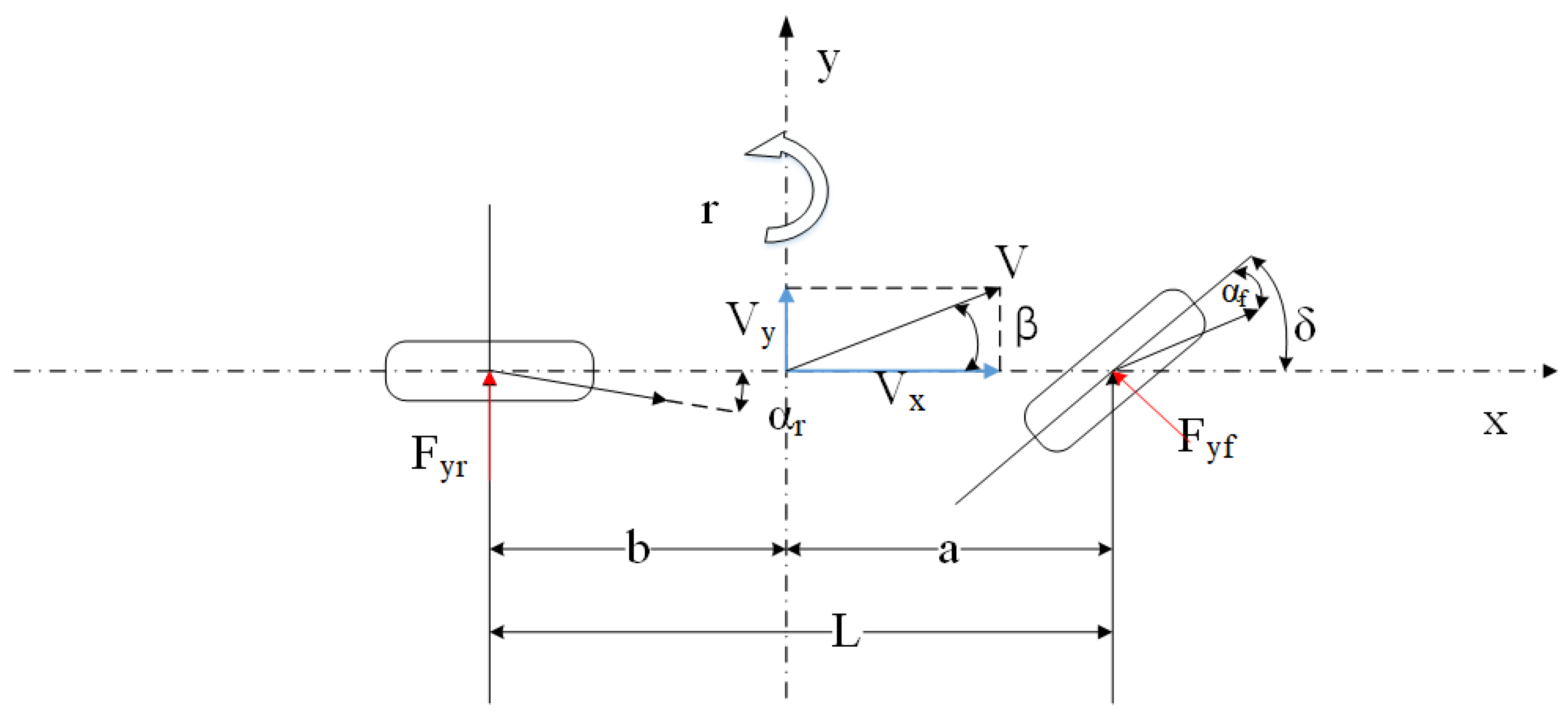
We consider a 2-DOF vehicle model, which is widely adopted to describe the vehicle’s lateral and yaw motion. The vehicle two-degrees-of-freedom model is shown in Figure 1. The assumptions considered in this model include the following:
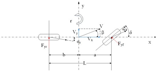
Figure 1.
2-DOF vehicle dynamics model.
- (1)
- Ignore the impact of the steering system and directly use the front wheel angle as input.
- (2)
- Ignore the effect of suspension; it is considered that the car compartment only moves in a plane parallel to the ground.
- (3)
- The forward speed of the vehicle along the x-axis is considered constant.
- (4)
- The driving force is not large, and the impact of tangential ground forces on tire cornering characteristics is not considered.
- (5)
- There is no aerodynamic effect, and the changes in tire cornering characteristics caused by load changes on the left and right tires and the effect of tire alignment torque are ignored.
The state space equations of the model are:
Lateral motion:
Yaw motion:
where is the vehicle mass; and are longitudinal and lateral velocities of CG; is the lateral tire force of the front wheels; is the lateral tire force of the rear wheels; is the moment of inertia of the vehicle; the yaw rate velocity of the vehicle; is the front and steering angles; are the sideslip angles of the front and rear wheels; is the wheelbase of the front and rear axles; is the distance from the center of mass to the front axle; is the distance from the center of mass to the rear axle.
Two tire models are used to verify the effectiveness of the algorithm: the linear tire model and the nonlinear model.
The linear tire model is as follows:
where is the tire cornering stiffness.
The front and rear wheel side slip angle are:
Equations (3)–(5) are combined with (1) and (2) to obtain a linear two-degrees-of-freedom model:
where is the angular acceleration of the sideslip angle of the center of mass, and is yaw angular acceleration. and represent the cornering stiffness of the front and rear axle.
The nonlinear tire model:
where are tire model parameters. The arctangent tire model is easy to design and solve for estimators and can also have good fitting accuracy in the area of sideslip angle before the tire reaches the adhesion limit.
Among them, are the front and rear wheel tangent model parameters, respectively.
3. Proposed Vehicle State Observer Based on RBF and Kalman Filter
The sideslip angle of a vehicle is a fundamental parameter, and its knowledge is the foundation of vehicle lateral stability control. The sideslip angle of a vehicle is the angle between the direction of travel and the direction of the vehicle, defined as:
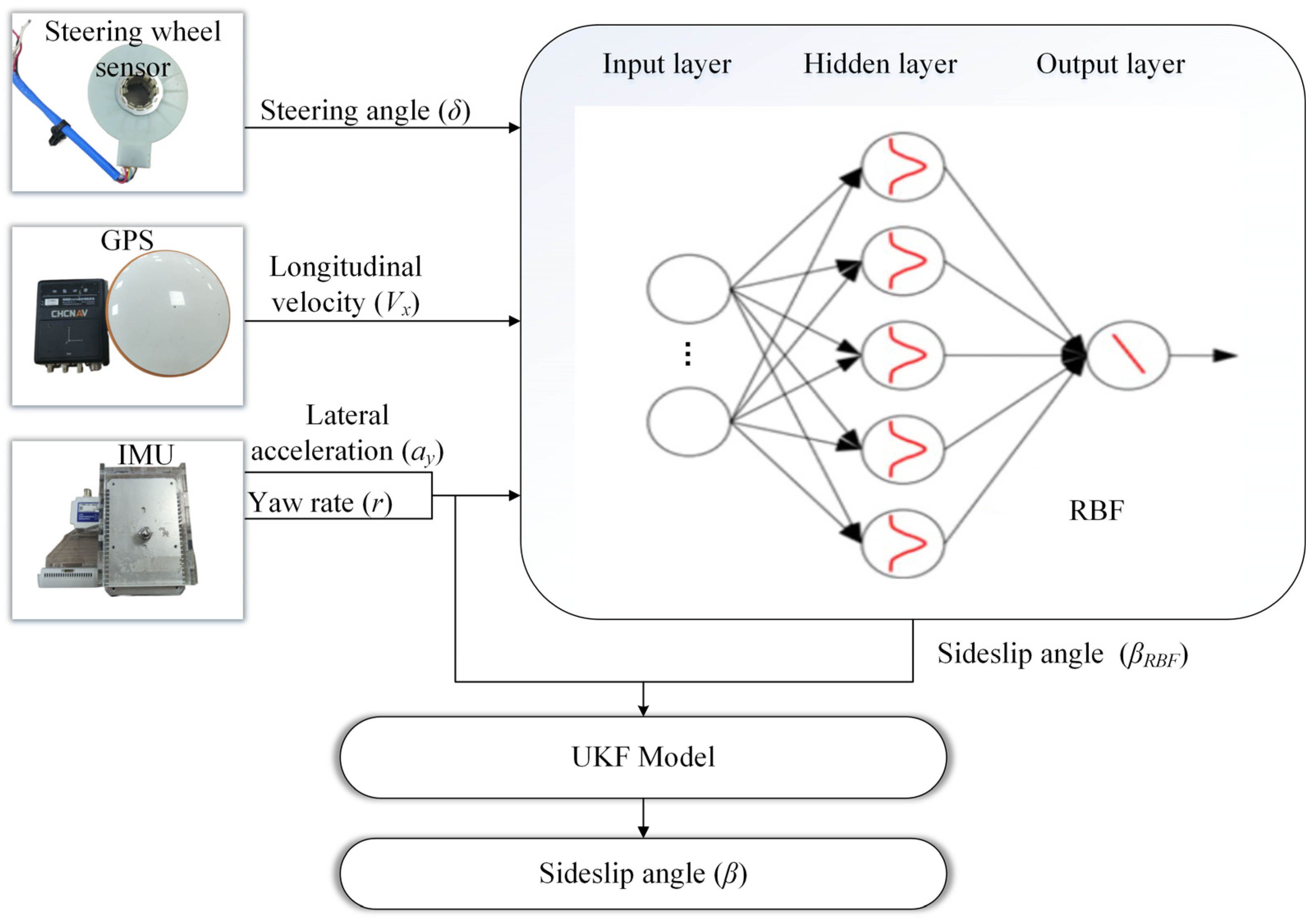
This article introduces a new fusion estimation algorithm to estimate sideslip angles. The structure of this fusion estimation method is shown in Figure 2.
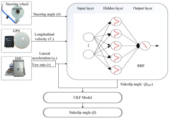
Figure 2.
Estimator architecture.
The former is an estimator based on RBF neural networks, which can estimate the centroid sideslip angle (pseudo sideslip angle). The input for this section is the steering angle measured by the steering wheel angle sensor, as well as the longitudinal velocity measured using GPS and the longitudinal acceleration and yaw rate measured using the IMU inertial measurement unit. The advantage of this observer is to use existing sensors in the vehicle for measurement. The observer based on RBF outputs a “Pseudo sideslip angle”, which serves as the input for the second part. Because this “Pseudo sideslip angle” is affected by noise, it cannot be directly used as a reference variable for vehicle lateral control. Therefore, we need the second part to filter out the impact of noise.
The second part is the Kalman filter. The module takes the lateral acceleration and yaw rate measured by IMU and the “pseudo sideslip angle” as the observations and combines the two-degrees-of-freedom model to obtain the final sideslip angle.
Finally, in the update stage of the Kalman filter, a new centroid sideslip angle is obtained to minimize the estimation error and obtain the optimal estimation value. To demonstrate the effectiveness of the proposed filtering algorithm, different Kalman filters (Kalman filter, extended Kalman filter, unscented Kalman filter) are considered.
3.1. Radial Basis Function Neural Network
RBF neural networks have attracted much attention due to their excellent generalization ability, simple network structure, and fast training speed. At the same time, relevant research also shows that RBF neural networks can approximate any nonlinear function with any precision [31,32].
The factors considered in selecting inputs for the RBF algorithm are the minimum type of input data; data that can be measured by the sensors included in the vehicle body are selected.
As well as from Equations (4) and (7), it can be seen that:
Assume is a constant:
We can think that:
In summary, the following types of data are selected as inputs for the neural network: yaw rate (), longitudinal velocity (), steering angle (), lateral acceleration ().
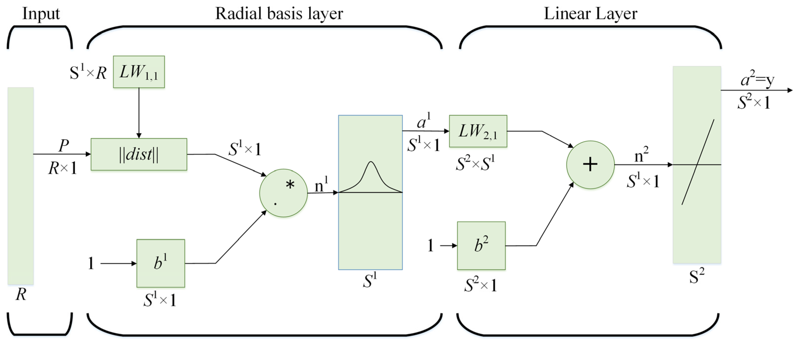
The RBF neural network has two layers: the hidden layer and the linear layer. Its structure is shown in Figure 3.
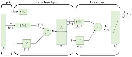
Figure 3.
Radial basis function neural network architecture.
Where denotes a single input vector and the matrix denotes a matrix consisting of input vectors.
Hidden layer: The neuron activation function of the hidden layer is composed of radial basis functions. The array operation units composed of hidden layers are called hidden layer nodes. The hidden layer node contains a center vector ; and the input parameter vector have the same dimension, and the Euclidean distance between them is defined as .
Among them, is a positive scalar representing the width of the Gaussian basis function; is the number of neurons in the hidden layer, 1 denotes the hidden layer, and is the results calculated by the hidden layer.
The output of the network is implemented using the following weighting function:
Among them, is neuron thresholds of linear layers, is the weight of the linear layer, : is the number of neurons in the linear layer, 2 denotes the linear layer, and is the output of linear layers.
In this paper, Matlab’s built-in radial basis neural network function was used to complete this work. The training process of the RBF neural network is shown in Figure 4. The four inputs mentioned in the above figure were selected for training to generate the required neural network model. At the same time, in order to prevent the algorithm from falling into local minima, a gradient descent method was used to obtain the number of hidden neurons, and finally, the optimal network was generated by testing the true values.
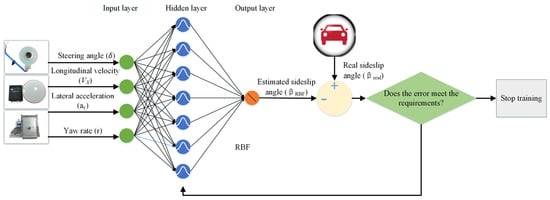
Figure 4.
RBF learning process.
The selection of a dataset is also very important, as it directly affects the effectiveness of neural networks. Therefore, for data selection, we hope that it can simultaneously represent both linear and nonlinear features of the vehicle while also demonstrating its responsiveness to different vehicle speeds.
One hundred and twenty J-turn conditions with different vehicle speeds and steering wheel angles were selected. The training data are shown in Table 1.

Table 1.
Set of simulation maneuvers for deep neural network training.
3.2. Kalman Filter Incorporating Radial-Based Neural Networks
3.2.1. Vehicle Dynamics Modeling for Estimator
The discrete nonlinear system of Kalman filtering can be represented as:
where and are nonlinear equations; represent the state vector; is the input vector; is the measurement vector; and are assumed to be white noise, zero mean, and uncorrelated:
where and are covariance matrices that describe the state and measurement noise.
By combining Equations (6) and (7), the state vector of the state space equation of the dynamic linear model, the measurement vector can be represented as follows:
By combining Equations (9) and (10), the state vector of the state space equation of the dynamic nonlinear model, the measurement vector can be represented as follows:
3.2.2. Radial Basis Neural Networks and Linear Kalman Filtering
When Equations (18) and (19) are linear, the state equation and measurement equation of the vehicle two degrees of freedom can be expressed as follows:
where matrices , .
To estimate the vehicle sideslip angle, Equations (20) and (21) are used as the state space equation and the measurement equation. The algorithmic process based on a radial basis neural network with Kalman filter is shown in Algorithm 1, where lines 6–10 are the standard Kalman filter process, is the neural network model, represents the sensor value sets for second as explained in Section 3.1, and is the output of the neural network model. The measurement vectors and covariance matrices (3–5 lines), matrices and matrices , are updated as follows:
| Algorithm 1 Radial Basis Neural Networks and Kalman Filtering. | |
| 1. | Function) |
| 2. | Basic parameter input |
| 3. | |
| 4. | |
| 5. | |
| 6. | |
| 7. | |
| 8. | |
| 9. | |
| 10. | |
| 11. | |
| 12. | Return |
3.2.3. Radial Basis Neural Networks with Extended Kalman Filtering
Extended Kalman filtering involves first-order Taylor expansion of the nonlinear state equation around the . The Equations (18) and (19) can be described as:
In the equations, , are the second-order or higher-order terms of the Taylor series of the nonlinear state function at the filtered value , and are the Jacobian matrices of and .
where is the time interval between two data.
In order to estimate the vehicle sideslip angle, Equations (22) and (23) are used as state space equations and measurement equations. The algorithmic process based on a radial basis neural network with an extended Kalman filter is shown in Algorithm 2, where lines 6–10 are the standard extended Kalman filter process and lines 3–5 are the same as the same steps described in Algorithm 1. The new measurement vector and covariance are as in Algorithm 1. The new matrix is shown below:
| Algorithm 2 Radial Basis Neural Networks and Extended Kalman Filtering. | |
| 1. | Function) |
| 2. | Basic parameter input |
| 3. | |
| 4. | |
| 5. | |
| 6. | |
| 7. | |
| 8. | |
| 9. | |
| 10. | |
| 11. | |
| 12. | Return |
3.2.4. Radial Basis Neural Networks with Unscented Kalman Filtering
Unscented Kalman filtering abandons the traditional practice of linearization of nonlinear functions and adopts a linear filtering framework. For the one-step prediction equation, the unscented transformation is used to deal with the nonlinear transfer problem of mean and covariance. The UKF approximates the probability density distribution of the nonlinear function and uses a series of determined samples to approximate the posterior probability density of the state.
The Equations (18) and (19) can be expressed as follows:
The UKF first defines sigma points and then passes them to nonlinear functions. The mean and covariance of Gaussian are recovered by using the passed sigma points. The sigma points are defined symmetrically to the mean of the Gaussian as follows:
where , and are scaling parameters that determine how far the sigma points from the mean would be.
In order to recover the mean and the covariance of the Gaussian from the sigma points, each sigma point is given a weight as follows:
where is the parameter containing prior information of the distribution.
Here, the mean and the covariance of the Gaussian distribution after the nonlinear function, , can be recovered from the passed sigma points, and the weights, as shown in Equation (38).
To estimate the vehicle sideslip angle, Equations (22) and (23) are used as the state space equation and the measurement equation. The algorithmic process based on a radial basis neural network with a traceless Kalman filter is shown in Algorithm 3, where lines 6–16 are the standard unscented Kalman filter process, and lines 3–5 are the same description of the same steps as in Algorithm 1. is the neural network model, and is the output of the neural network model.
| Algorithm 3 Radial Basis Neural Networks and Unscented Kalman Filtering. | |
| 1. | Function) |
| 2. | Basic parameter input |
| 3. | |
| 4. | |
| 5. | |
| 6. | |
| 7. | |
| 8. | |
| 9. | |
| 10. | |
| 11. | |
| 12. | |
| 13. | |
| 14. | |
| 15. | |
| 16. | |
| 17. | Return |
4. Results
Carsim 2020 software has been proven to be used to verify the effectiveness of the algorithm. Therefore, Carsim 2020 software was used to obtain relevant experimental data to prove the proposed RBF joint Kalman filter algorithm.
Since the real experimental data always have noise interference, we added Gaussian noise with a mean of zero and a variance of 0.01°, 0.01°/s, 0.01 m/s2, and 0.01 km/h to the steering wheel angle, yaw rate, lateral acceleration, and longitudinal velocity obtained by Carsim 2020.
The vehicle model is a C-class hatchback car, and the tire model is 205/45 R17. The interval between the two data is 0.025 s. The hardware configuration we used is CPU 2.5 G HZ, no GPU, and an 8 GB memory module. Table 2 shows the parameters of the vehicle.
Table 2.
Vehicle of parameters for the C-Class hatchback car.
The effectiveness and strong robustness of the designed estimator are demonstrated by estimating the sideslip angle of vehicles under different operating conditions, as shown in Table 3. Firstly, there are four types of double lane changing conditions, and the 1.2 conditions, respectively, demonstrate the effectiveness of the designed sideslip angle estimator in high speed with high adhesion and high speed with low adhesion states, and the 3.4 conditions show the effectiveness of the designed sideslip angle estimator in high and medium adhesion states at lower vehicle speeds. The 5.6 conditions are the high attachment, middle attachment, high-speed J-turn maneuver. The above vehicle speeds are fixed, and the test conditions are not included in the training process.
Table 3.
Experimental conditions for test dataset.
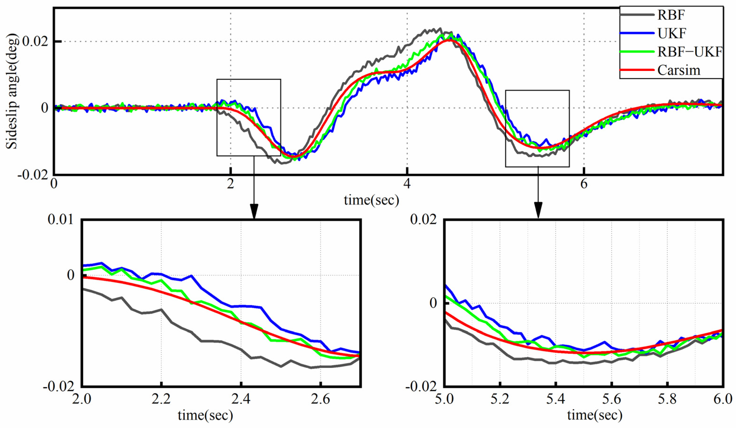
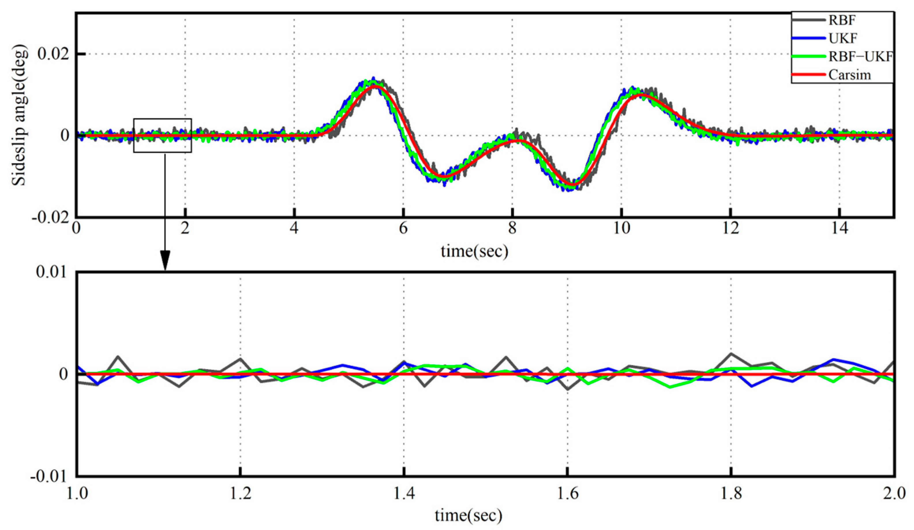
Figure 5 shows the comparison overall estimation results of the RBF-based observer, the UKF-based observer, and the RBF-UKF-based observer with the double lane changing maneuver on the road with a friction coefficient of 0.85 at a speed of 100 km/h. It is seen that the three observers of RBF, UKF, and RBF-UKF can better reflect the changing trend of the actual vehicle sideslip angle, but their estimation accuracy is very different. RBF, compared with UKF and RBF-UKF, always presents the characteristics of larger and earlier changes to the expected results. The estimated value of the UKF observer is greater than the reference value in the range of 2.0~2.6 s and 5.0~5.5 s, and the estimated value is less than the reference value in the range of 3.5~4.5 s. The observation results of the RBF-UKF observer in the limit state are closer to the reference value. From a numerical point of view, the maximum errors of the observer based on RBF, UKF, and RBF-UKF observers are 0.0080, 0.0069, and 0.0061, respectively. The root mean square errors of the three observers are 0.0027, 0.0023, and 0.0016, respectively. The root mean square error and maximum error of the RBF-UKF observer are the smallest.
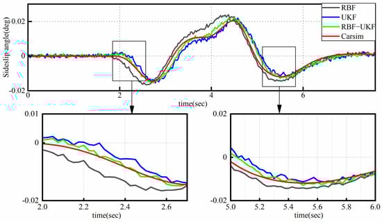
Figure 5.
Results for sideslip angle estimation for condition 1.
Figure 6 shows a double lane changing operation at a speed of 100 km/h on a road with a friction coefficient of 0.3. This condition shows that the proposed observer cannot provide the required force of the vehicle, that is, the observation effect under the out-of-control state. We can see that the RBF observer can roughly reflect the changing trend of the actual sideslip angle of the vehicle, but the estimation accuracy of the sideslip angle in −0.025~−0.01 and 0.015~0.03 (large sideslip angle or limit state) is still insufficient. Based on UKF, the estimation results of RBF-UKF observer have no reference value. The maximum errors of the observer based on RBF, UKF, and RBF-UKF observers are 0.0189, 0.0696, and 0.0587, respectively. The root mean square errors of the three observers are 0.0086, 0.0273, and 0.0237, respectively.
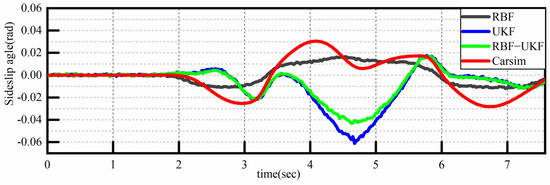
Figure 6.
Results for sideslip angle estimation for condition 2.
Figure 7 shows the results for a vehicle traveling a double line changing at 50 km/h on a road surface with a friction coefficient of 0.85. The figure shows that the observation accuracy of all three observers exhibits good observation accuracy at medium speed and high attachment; when there is noise input, the UKF and RBF-UKF observers using the filtering algorithms show significantly less fluctuation in the estimation compared to the RBF-based observer to obtain the sideslip angle. The root-mean-square errors based on RBF, UKF, and RBF-UKF are 0.0011, 0.0016, and 0.0012, respectively. The maximum errors are 0.0041, 0.0050, and 0.0048, respectively.
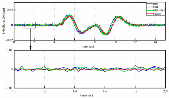
Figure 7.
Results for sideslip angle estimation for condition 3.
Figure 8 shows that the vehicle performs a J-turn at a speed of 100 km/h on a road with a road adhesion coefficient of 0.85. The diagram shows that the three observers have good estimation results for the sideslip angle of the vehicle after entering the steady state (2–10 s), but the estimation results of the RBF observer are more consistent with the reference value; when the steering wheel suddenly changes and is fixed to a specific value, the transient change in the vehicle sideslip angle (0–1 s), the three observers do not show good estimation results; the UKF-RBF observer has a better observation effect during 1~2 s. The root of mean square errors of RBF, UKF, and RBF-UKF are 0.0055, 0.00106, and 0.0052, respectively, and the maximum errors are 0.0248, 0.0287, and 0.0248, respectively. According to these data, RBF-UKF fits the data better for the whole working condition.

Figure 8.
Results for sideslip angle estimation for condition 5.
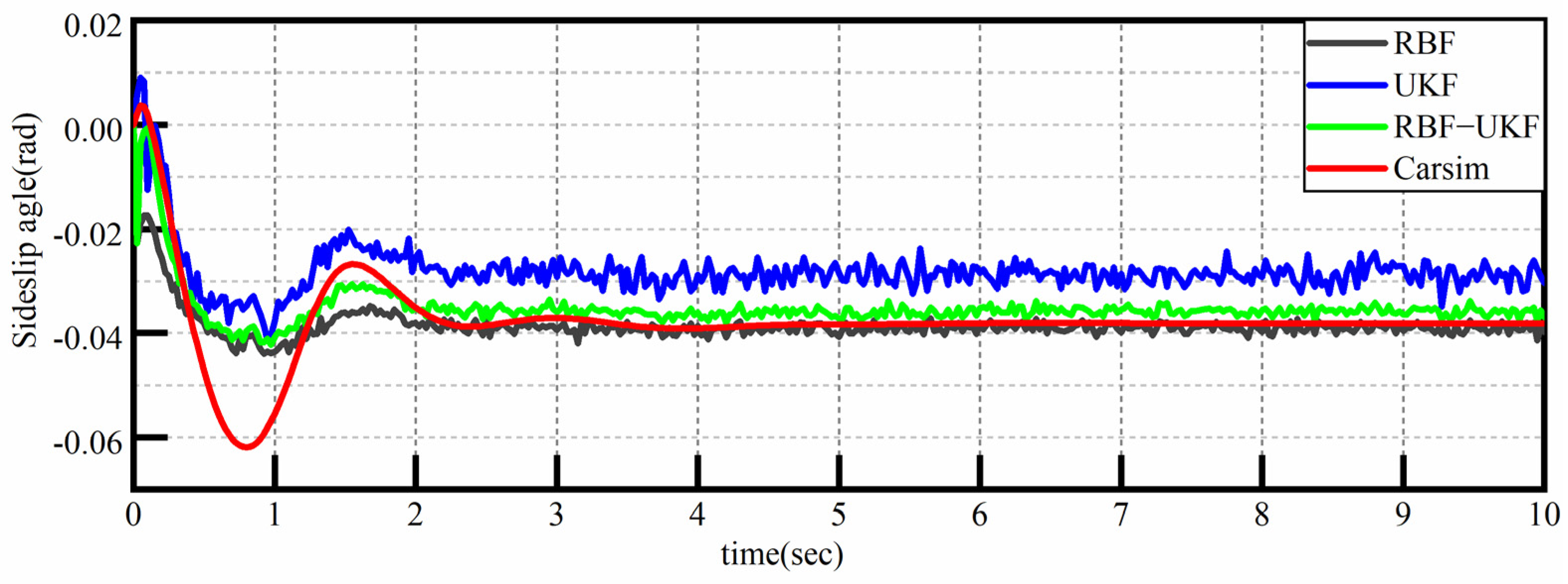
Figure 9 shows that the vehicle performs a J-turn at a speed of 100 km/h on a road with a road adhesion coefficient of 0.5, and the estimated results of the RBF-UKF observer are more consistent with the reference values. RBF observer shows poor estimation of performance. The root of mean square errors of RBF, UKF, and RBF-UKF are 0.0139, 0.0150, and 0.0090, respectively, and the maximum errors are 0.0255, 0.0423, and 0.0343, respectively.
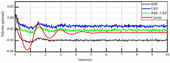
Figure 9.
Results for sideslip angle estimation for condition 6.
From the results, we can conclude that the proposed observer based on RBF-UKF achieves a better estimation of the sideslip angle.
In order to compare the performance, the root mean square error (RMSE) and the maximum error (Emax) are chosen. It has been shown that Kalman filtering is necessary to reduce noise measurements. From Table 4, it can be concluded that the root means square error of RBF-UKF is reduced by 0.0009 (Con.1), 0.001 (Con.4), 0003 (Con.5), and 0.0049 (Con.6) in comparison to RBF. The root means square error of RBF-UKF is reduced by 0.0007 (Con.1), 0.0004 (Con.3), 0.0003 (Con.4), 0.0054 (Con.5), and 0.006 (Con.6), respectively, as compared to UKF. Meanwhile, the root means square error of RBF-EKF is reduced by 0.0001 (Con.3) compared to that of RBF-UKF. Table 5 shows that RBF-EKF reduces the maximum error by 0.0006 (Con.1) and 0.0013 (Con.3) compared to RBF-UKF. In the whole test scenario, all observers fusing neural networks with Kalman filtering algorithms show better performance compared to considering RBF or Kalman algorithms alone. The RBF-UKF-based observer provides better or the same performance compared to other Kalman-based observers (RBF-KF, RBF-EKF). In some cases, the RBF-EKF observer achieves better results than RBF-UKF, but it does not achieve a significant advantage in terms of overall working conditions.
Table 4.
Root means square error of different test conditions (RMSE).
Table 5.
Maximum error for different test conditions (Emax).
5. Conclusions
In this paper, a new RBF-UKF estimator is used to estimate the sideslip angle. The value of the “pseudo sideslip angle” is obtained by the neural network model, and the information is combined with the Kalman filter based on the dynamic model. The estimator fully integrates the advantages of the neural network and vehicle two-degrees-of-freedom model, which solves the generalization difficulty caused by the lack of training data of the neural network and also solves the accuracy problem of the two-degrees-of-freedom model under certain working conditions. At the same time, the Kalman filter algorithm can also effectively reduce the interference of the estimation process noise. The model trained by the neural network is still biased toward the effect of the vehicle dynamics model. In the state of the vehicle out of control, the RBF-based filtering algorithm cannot accurately estimate the magnitude of the sideslip angle under extreme operating conditions, and the RBF-UKF estimator cannot effectively estimate the vehicle sideslip angle. The model has been verified by a set of working conditions representing different test conditions. Compared with the observer based on RBF and different Kalman filters, the RBF-UKF observer can more accurately reflect the change in vehicle sideslip angle.
6. Prospect
For neural network models, a high-precision vehicle simulation model can be constructed to generate ideal network training signals suitable for various driving situations to compensate for data deficiencies; in order to improve the robustness of the estimator, future research can attempt to estimate the real-time state of the vehicle or reduce the credibility of the dynamic state equation by incorporating kinematics in the state of runaway. At the same time, future research can attempt to use real-world vehicles for experiments.
Author Contributions
Conceptualization, C.Z., Y.F. and P.Q.; methodology, C.Z.; software, Y.F.; validation, C.Z., Y.F. and J.W.; formal analysis, P.G.; investigation, C.Z.; resources, C.Z.; data curation, C.Z. and P.Q.; writing—original draft preparation, Y.F.; writing—review and editing, P.G.; visualization, J.W.; supervision, J.W.; project administration, C.Z.; funding acquisition, C.Z. All authors have read and agreed to the published version of the manuscript.
Funding
This research was funded by the Shaanxi Innovation Talent Promotion Plan—Science and Technology Innovation Team (2021TD-27) and the 2022 Youth Innovation Team Construction Scientific Research Program of Shaanxi Provincial Education Department (22JP045).
Data Availability Statement
Not applicable.
Conflicts of Interest
The authors declare no conflict of interest.
References
- Suzuki, Y.; Takeda, M. An overview on vehicle lateral dynamics and yaw stability control systems. J. Adv. Vehic. Eng. 2016, 2, 182–190. [Google Scholar]
- Tang, X.; Yan, Y.; Wang, B.; Xu, X.; Zhang, L. Analysis of Intrinsic Mechanistic of Stability-Tracking Control for Distributed Drive Autonomous Electric Vehicle. Electronics 2021, 10, 3010. [Google Scholar] [CrossRef]
- Bengler, K.; Dietmayer, K.; Farber, B.; Maurer, M.; Stiller, C.; Winner, H. Three decades of driver assistance systems: Review and future perspectives. IEEE Intell. Transp. Syst. Mag. 2014, 6, 6–22. [Google Scholar] [CrossRef]
- Sun, B.; Zhang, T.; Gao, S.; Ge, W.; Li, B. Design of brake force dis-tribution model for front-and-rear-motor-drive electric vehicle based on radial basis function. Arch Transp. 2018, 48, 87–98. [Google Scholar] [CrossRef]
- Guo, H.; Cao, D.; Chen, H.; Lv, C.; Wang, H.; Yang, S. Vehicle dynamic state estimation: State of the art schemes and perspectives. IEEE/CAA J. Autom. Sin. 2018, 5, 418–431. [Google Scholar] [CrossRef]
- Chindamo, D.; Lenzo, B.; Gadola, M. On the vehicle sideslip angle estimation: A literature review of methods, models, and innovations. Appl. Sci. 2018, 8, 355. [Google Scholar] [CrossRef]
- Xiong, L.; Xia, X.; Lu, Y.; Liu, W.; Gao, L.; Song, S.; Yu, Z. IMU-based automated vehicle body sideslip angle and attitude estimation aided by GNSS using parallel adaptive Kalman filters. IEEE Trans. Veh. Technol. 2020, 69, 10668–10680. [Google Scholar] [CrossRef]
- Liu, W.; Xia, X.; Xiong, L.; Lu, Y.; Gao, L.; Yu, Z. Automated vehicle sideslip angle estimation considering signal measurement characteristic. IEEE Sens. J. 2021, 21, 21675–21687. [Google Scholar] [CrossRef]
- Xia, X.; Xiong, L.; Lu, Y.; Gao, L.; Yu, Z. Vehicle sideslip angle estimation by fusing inertial measurement unit and global navigation satellite system with heading alignment. Mech. Syst. Signal Process. 2021, 150, 107290. [Google Scholar] [CrossRef]
- Du, H.; Zhang, N.; Dong, G. Stabilizing vehicle lateral dynamics with considerations of parameter uncertainties and control saturation through robustyaw control. IEEE Trans. Veh. Technol. 2010, 59, 2593–2597. [Google Scholar]
- Guo, H.; Chen, H.; Cao, D.; Jin, W. Design of a reduced-order non-linear observer for vehicle velocities estimation. IET Control. Theory Appl. 2013, 7, 2056–2068. [Google Scholar] [CrossRef]
- Kim, J. Effect of vehicle model on the estimation of lateral vehicle dynamics. Int. J. Automot. Technol. 2010, 11, 331–337. [Google Scholar] [CrossRef]
- Wenzel, T.A.; Burnham, K.; Blundell, M.; Williams, R. Dual extended kalman filter for vehicle state and parameter estimation. Veh. Syst. Dyn. 2006, 44, 153–171. [Google Scholar] [CrossRef]
- Huang, X.; Wang, J. Robust sideslip angle estimation for lightweight vehicles using smooth variable structure filter. In Proceedings of the 2013 ASME Dynamic Systems and Control Conference, Palo Alto, CA, USA, 21–23 October 2013. [Google Scholar]
- Davoodabadi, I.; Ramezani, A.A.; Mahmoodi-k, M.; Ahmadizadeh, P. Identification of tire forces using Dual Unscented Kalman Filter algorithm. Nonlinear Dyn. 2014, 78, 1907–1919. [Google Scholar] [CrossRef]
- Guo, K.H.; Lei, R. A Unified Semi-Empirical Tire Model with Higher Accuracy and Less Parameters; SAE: Warrendale, PA, USA, 1999. [Google Scholar]
- Li, L.; Jia, G.; Ran, X.; Song, J.; Wu, K. A variable structure extended kalman filter for vehicle sideslip angle estimation on a low friction road. Veh. Syst. Dyn. 2014, 52, 280–308. [Google Scholar] [CrossRef]
- Bechtoff, J.; Isermann, R. Cornering stiffness and sideslip angle estimation for integrated vehicle dynamics control. IFAC-PapersOnLine 2016, 49, 297–304. [Google Scholar] [CrossRef]
- Mosconi, L.; Farroni, F.; Sakhnevych, A.; Timpone, F.; Gerbino, F.S. Adaptive vehicle dynamics state estimator for onboard automotive applications and performance analysis. Veh. Syst. Dyn. 2022, 1–25. [Google Scholar] [CrossRef]
- Xia, X.; Hashemi, E.; Xiong, L.; Khajepour, A. Autonomous vehicle kinematics and dynamics synthesis for sideslip angle estimation based on consensus kalman filter. IEEE Trans. Control. Syst. Technol. 2022, 31, 179–192. [Google Scholar] [CrossRef]
- Lee, H. Reliability indexed sensor fusion and its application to vehicle velocity estimation. J. Dyn. Sys. Meas. Control. 2006, 128, 236–243. [Google Scholar] [CrossRef]
- Saadeddina, K.; Abdel-Hafezd, M.F.; Jaradatb, M.A.; Jarrahd, M.A. Performance enhancement of low-cost, high-accuracy, state estimation for vehicle collision prevention system using ANFIS. Mech. Syst. Signal Process. 2013, 41, 239–253. [Google Scholar] [CrossRef]
- Du, H.; Zhang, N. Robust Vehicle Stability Control Based on Sideslip Angle Estimation. In Robust Control Theory and Applications; Bartos-zewicz, A., Ed.; InTech: Rijeka, Croatia, 2011; ISBN 978-953-307-229-6. [Google Scholar]
- Melzi, S.; Sabbioni, E. On the vehicle sideslip angle estimation through neural networks: Numerical and experimental results. Mech. Syst. Signal Process. 2011, 25, 2005–2019. [Google Scholar] [CrossRef]
- Boada, B.L.; Boada, M.J.L.; Gauchía, A.; Olmeda, E.; Díaz, V. Sideslip angle estimator based on ANFIS for vehicle handling and stability. J. Mech. Sci. Technol. 2015, 29, 1473–1481. [Google Scholar] [CrossRef]
- Wei, W.; Shaoyi, B.; Lanchun, Z.; Kai, Z.; Yongzhi, W.; Weixing, H. Vehicle sideslip angle estimation based on general regression neural network. Math. Probl. Eng. 2016, 2016, 3107910. [Google Scholar] [CrossRef]
- Shaohua, L.; Guiyang, W.; Zekun, Y.; Xuewei, W. Dynamic joint estimation of vehicle sideslip angle and road adhesion coefficient based on DRBF-EKF algorithm. Li Xue Xue Bao 2022, 54, 1853–1865. [Google Scholar]
- Boada, B.; Boada, M.; Diaz, V. Vehicle sideslip angle measurement based on sensor data fusion using an integrated anfis and an unscented kalman filter algorithm. Mech. Syst. Signal Process. 2016, 72, 832–845. [Google Scholar] [CrossRef]
- Kim, D.; Min, K.; Kim, H.; Huh, K. Vehicle sideslip angle estimation using deep ensemble-based adaptive Kalman filter-ScienceDirect. Mech. Syst. Signal Process. 2020, 144, 106862. [Google Scholar] [CrossRef]
- Tommaso, N.; Renzo, C.; Claudio, A. An integrated artificial neural network–unscented Kalman filter vehicle sideslip angle estimation based on inertial measurement unit measurements. Proc. Inst. Mech. Eng. Part D J. Automob. Eng. 2018, 233, 095440701879064. [Google Scholar]
- Hartman, E.J.; Keeler, J.D.; Kowalski, J.M. Layered neural networks with Gaussian hidden units asuniversal approximations. Neural Comput. 1990, 2, 210–215. [Google Scholar] [CrossRef]
- Park, J.; Sandberg, L.W. Universal approximation using radial-basis-function networks. Neural Comput. 1991, 3, 246–257. [Google Scholar] [CrossRef]


Disclaimer/Publisher’s Note: The statements, opinions and data contained in all publications are solely those of the individual author(s) and contributor(s) and not of MDPI and/or the editor(s). MDPI and/or the editor(s) disclaim responsibility for any injury to people or property resulting from any ideas, methods, instructions or products referred to in the content. |
© 2023 by the authors. Licensee MDPI, Basel, Switzerland. This article is an open access article distributed under the terms and conditions of the Creative Commons Attribution (CC BY) license (https://creativecommons.org/licenses/by/4.0/).