Mathematical Modeling of a Multi-Chamber Pneumatic Soft Actuator

Abstract

Owing to their compliance with most shapes, soft actuators are regarded as cost-effective solutions for grasping irregular objects. The material properties of nonlinear elastic polymers are considered necessary for the correct implementation of these actuators. The analysis tends to be complex even for simple movements defined by theoretically infinite degrees of freedom. This study offers a mathematical model that outlines a relationship between the energy provided by a pressure source and the expected behavior of multi-chamber pneumatic soft actuators through hyper-elastic material deformation interpretation, geometric approximations, and the vectorial representations of their segments. Digitally analyzed empirical results measured through lateral pictures of an actuator were taken at different pressure references. Direct comparisons between the average value of the tested angles and those calculated through the tuned mathematical model provide a maximum error of 0.647° for small deformations and an improved accuracy at higher pressure inputs. This study offers a valid tool applicable to the design of soft actuators and their further analysis without the need for overly complex methods.

1. Introduction

As an innovative outlook on the nature of the material properties of robotic components, the field of soft robotics offers beneficial attributes through its compliance for irregular surfaces and delicate yet effective grip of fragile objects. Throughout the course of its development, diverse control and actuation methods have been devised, ranging from the use of thermally manipulated materials to engineered geometric designs for the deformation of soft bodies [1]. Having established a system determined by an objective task, the study of soft actuators coursed into defining mechanisms for movements such as radial expansion, longitudinal elongation, rotation and flexion [2,3]. When faced specifically with a pneumatically controlled system, the parameters of importance stand primarily in the geometry of both internal and external elements. Thus, a systematic response can be expected using a set shape, material, width, and air pressure source for a soft robotic device [4,5]. Stating a flexion-type actuator, the principle of its movement is primarily given by one or more internal chambers shifted from the center of inertia given by the transverse area of the body [6,7].

The differentiation between actuation types presents different applications for mechanical projects. The use of soft robotics can range from a simple one-degree-of-freedom mechanism to multiple-degrees-of-freedom robots. Complex soft robots tend to be inspired by biological mechanisms and their objectives can be applied toward engineering design [8]. Further complexity allows their functionality in various mediums.

For the control of a pneumatic soft actuator, the core components will be a pressure source, an enabling mechanism, a pressure-regulating piece and distribution channels [9,10,11]. Most of the components tend to be discreet in nature but the air flow rate, given by the energy source, determines the dynamic responses of the body and correlates directly to variables such as the manometric pressure [12]. Although closed-loop systems are generally superior in most cases, they are considerably demanding for implementation in soft actuators owing to their fast change of state and low measurable differences in common variables [13]. Closed-control systems are usually implemented as tools of analysis whereas the determination of specific inputs and their relation to the output through testing or modelling is the predetermined method of practical execution [9].

A general consensus for the manufacturing of pneumatic soft robotics is the use of hyper-elastic materials, owing to their high range of deformation and tendency to return to their original state after a force has acted upon them; thus, it is necessary to implement a soft gripper and ensure its longevity [14]. Although their properties are useful, the analysis of hyper-elastic materials is troublesome, because they do not obey Hooke’s law for linear elasticity [15,16]. Various models with different degrees of approximation were formulated to create a relationship between the induced external energy and a nonlinear elastic material, most notoriously the Neo-Hookean and Mooney–Rivlin models [17]. These nonlinear elastic models prove to be a useful tool for soft robotics even with different methods of actuation. Methods such as the inclusion of ECF (electro-conjugate fluid) or other fluidic inputs create a new method for energy inputting, but the deformation of overall elastic mechanics is constantly defined [18,19].

The study of composite systems tends to yield complex equations regarding a continuous form of analysis through the entire body that is rendered inefficient for a discrete approximation and can be used [1]. Defining the elements of a soft body through mathematical means proves challenging in any design, and its implementation in a high-degree model of actuation increases the difficulty [20]. Resorting to the use of several, simpler models for the individual parts of a structure is prioritized in control systems and non-focused research efforts whereby accuracy is sacrificed for the sake of practicality. By contrast, in-depth research can highlight material properties, even when applying statistical methods to convey the behavior of an isolated unique body [21].

The representation of entire, three-dimensional bodies through concrete mathematical equations that are not dependent on numerical tools are not easily obtained. The use of a “Backbone Curve” defining the longest dimension of a soft body is advised [22]. The method for defining this trajectory can be devised in various ways as its consistency lies in the fact that any vector tangential to the curve will always be orthogonal to the transverse area of the body [23]. In the case of defined, geometrically restricted actuators, the practical representation is given by the use of linear vectors describing regions separated by critical points of interest that may be due to a particular interaction between a force and the material or because of geometric limitations [24,25].

Given the initial parameters of the body of a soft actuator, we can determine the movement and positioning of its vectorial components, thus providing a tool to determine the utility of certain designs [26]. To tie all individual segments together, recursive equations can serve as a means of creating a graphically represented finalized model [27]. This is a simple way of analyzing a system that will be as accurate as many inflexion points and critical areas there are [28].

The lack of a simple deterministic model with easily analyzed variables prevents ease of study in the field of soft robotics for researchers focusing on design and manufacturing. Design parameter choices are only set as estimations or require the use of numeric methods through complex software to determine the correct behavior intended. This article presents a simple model to define how the geometric design of multi-chamber soft actuators affects their positioning in relation to air flow input.

The rest of the article is ordered as follows: Section 2 describes the materials and methodology used throughout the process of obtaining results, Section 3 outlines the process behind the formulation of the complete mathematical model as well as numerical results, Section 4 offers a discussion comparing previous studies and their application and Section 5 renders the conclusions and interpretation of results.

2. Materials and Methods

This study is divided into subdomains for individual analysis. As a research frame of reference, the methodology used was hierarchical, where each section is interpreted separately and general relations between each governing group are established to finalize its congruence as a whole. Its main objective aims to satisfy the functionality requirements stated by the initially stated design parameters [29].

The mathematical model depicting a soft actuator’s trajectory and position was broken into three main categories: analysis of pressure and deformation, calculation of displacement caused by geometrical changes and angular representation using linear vectors as illustrated in Figure 1. Additionally, the auxiliary sections such as reference design, parameters, manufacturing and calculated test data comparison are used in the validation and practical use of the model. While each section was studied independently, their inputs and outputs are strongly related.

Taking the study of pressure as the main source of energy, a method to predict its effect on the body must be presented. A traditional physics approach is used towards calculating the energy produced by the system’s pressure, but its outcome is defined by means of the Neo-Hookean model for nonlinear elastic materials.

Once the energy of the system is stated, its effect presents geometrical alterations to specific parts of the body which creates movement. Although considered as an estimation, the use of geometry based on ellipses is the representation employed for deformation in the inner pneumatic chambers within the actuator. Furthermore, the use of a previous study introduced by J. Wang provided a clear relationship between the lateral measurement of deformation and the effect of a single chamber upon the flexion of the body of the actuator.

Using the information from previous calculations, the representation of a backbone curve depicting the actuator’s movement was fabricated using linear vectors. The half angles are relative only to their specific segments; thus, a series of recursive equations are used to define the global angle that dictates the direction of each component. A similar method was utilized to obtain the coordinates of their respective origins. Using the design parameters as their magnitudes, a complete representation is achieved.

Defining a discrete model where only geometric parameters and tangential behavior of adjacent ellipses are considered, derived from energetic and material studies, some assumptions must be stated. Upper, front and rear chamber walls will not be significantly deformed due to their width. Longitudinal deformation will not occur due to a lack in effective contact and the restriction layer usually introduced at its base. An actuator’s body is completely homogeneous on its elastomer distribution. Air flow input is controllable and constant. The actuator’s body is symmetric. The base is not wide enough to restrict movement. Most assumptions are addressed on the manufacturing and design process for conventional multi-chamber pneumatic soft actuators.

3. Results

3.1. Reference Design, Parameters and Manufacturing

To define a mathematical model, the physical phenomenon must be clearly defined as a grounding reference. The specific type of soft actuator analyzed in this study was a multi-chamber pneumatic soft actuator, meaning that its source of motion is entirely powered by air pressure. Its body is divided into multiple segments that are almost independent from one another. Even though they are powered by the same energy source, the effects of each chamber are determined only by the geometrical design with which they were manufactured. This leads to an individual study of each chamber, later to be interpreted as their effects on the system.

By minimizing the spacing between each chamber and resorting to a design containing seven active segments, pronounced flexion is ensured even at small relative pressures and perceivable chamber deformations. This proves beneficial from an informative point of view since results will be defined in a way that is easily distinguishable, providing ease in the formulation of eventual conclusions.

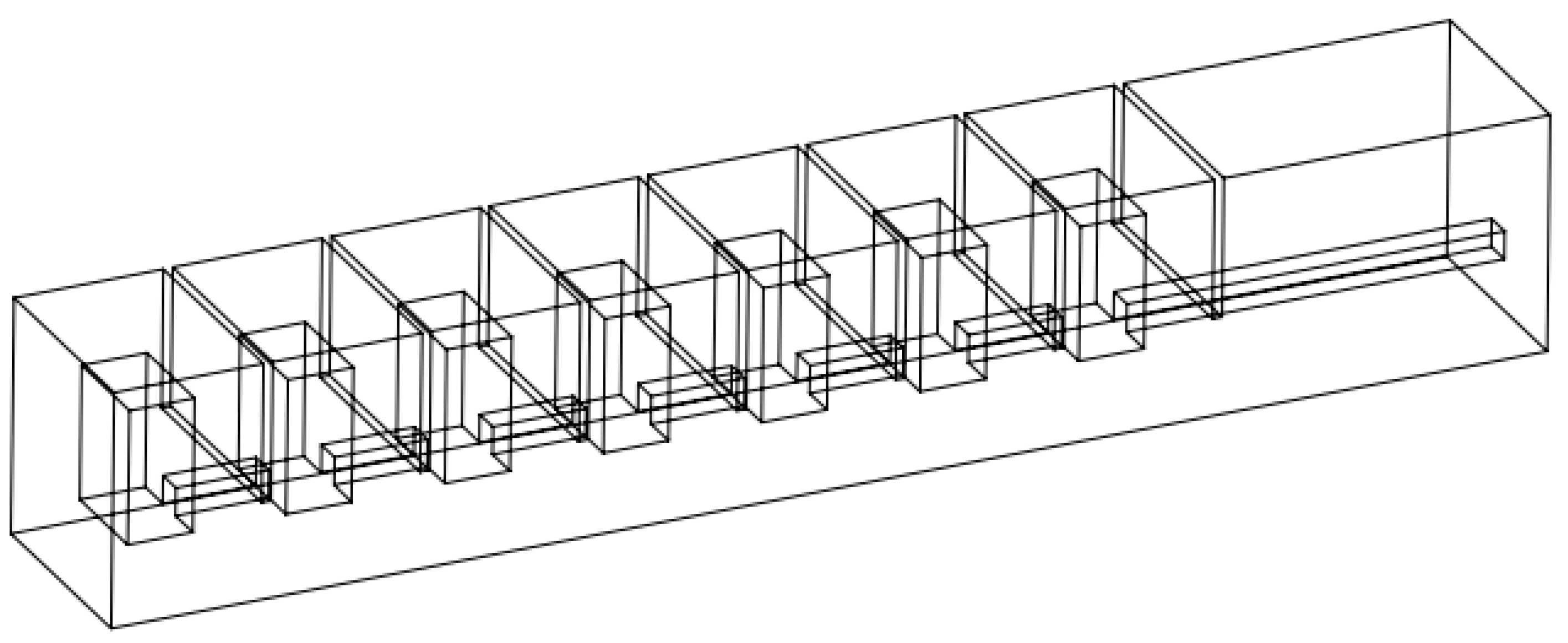
The design that was tested and validated throughout this study is presented in Figure 2, portraying its external and internal composition.

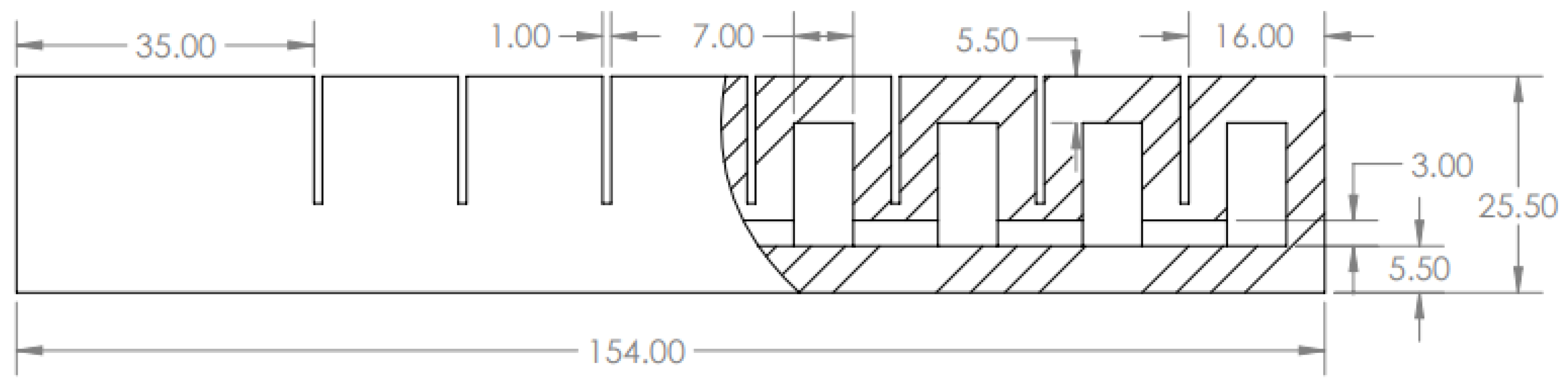
All the design parameters relevant to the mathematical model are described in Figure 3. These specific values were used to create a comparison between a real actuator and a prediction based on the mathematical model. Both the external part and the broken out section cut are presented.

The methodology offers a model that can be utilized with conventional actuators; with each measurement taken as an average from most common designs used industrially and for research purposes.

To manufacture the actuator’s component, an elastomer with hyper-elastic properties was selected. Given several factors, such as its elevated deformation coefficient, its cost and availability as well as its notorious resistance towards external piercing forces, ABRO GREY 999 RTV Silicone Gasket Maker was selected as the actuators body. Due to the models used to calculate elastic deformations, a shear modulus of only 18 GPa is required.

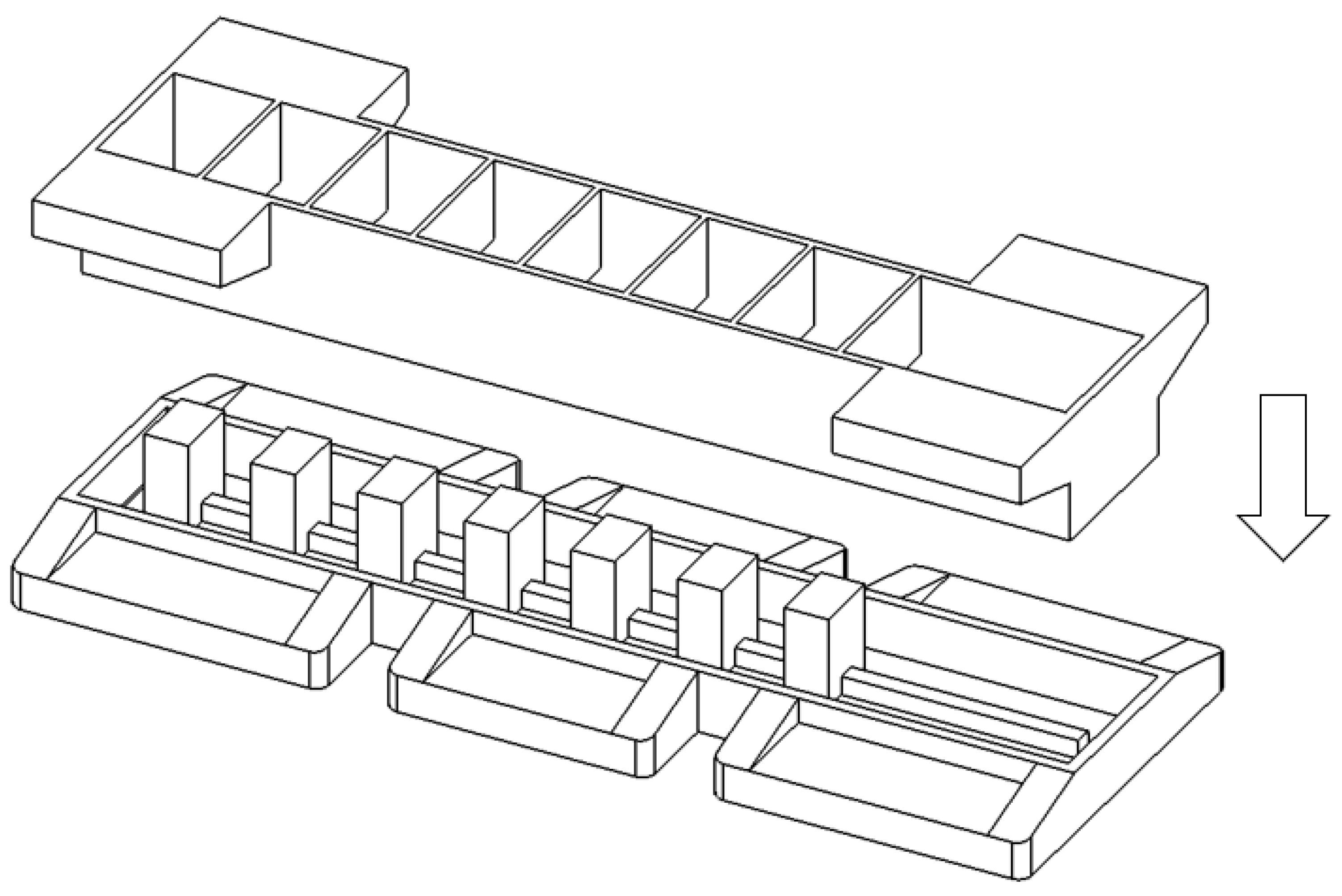
The entire process defines a multi-step traditional molding. Figure 4 presents both molds used to manufacture the body, only accounting for the chamber cavities and external separations.

After assembling both pieces, the material is poured, taking caution to avoid air bubbles because they affect the composition as a whole or can create air leaks which render the actuator nonfunctional. Due to the material’s properties, it is cured at room temperature across a period of 4 days to ensure its proper finishing. Figure 5 illustrates a fully cured actuator body ready to be released from its mold.

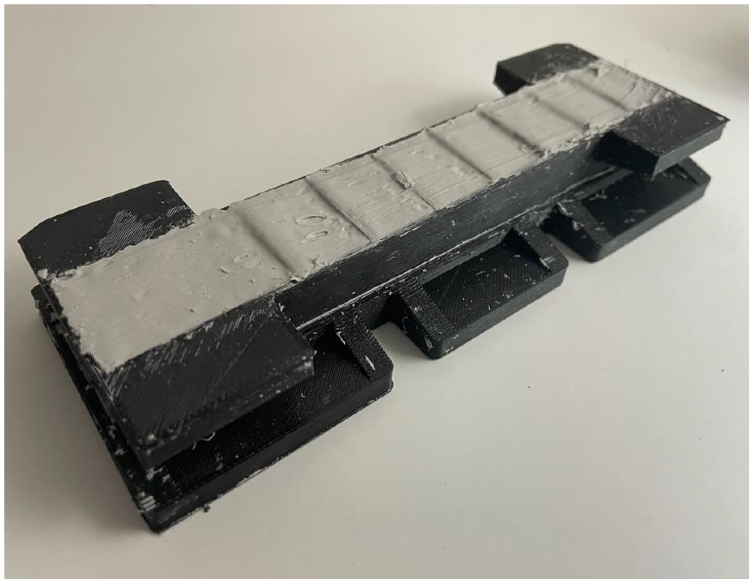
Once the body is removed from the mold, additional material is poured on a flat surface where the body will be laid on. The first layer of the base must be thin as to avoid clogging the main distribution channel. Curing time is 30 min for this step. A coupling method or direct source of distribution for air pressure should be introduced simultaneously making use of the materials own properties to create a seal. Addition at a later time could ultimately result in air leaks.

A layer of flexible but inelastic material should be applied at the latest layer of base material as an elongation limitation. More material poured over the inelastic layer creates an outer homogeneous composition and ensures the layers coupling towards the rest of the body. Multiple components can be manufactured and attached to a rigid assembly to finalize a proper functional actuator presented in Figure 6 in a three component configuration over an industrial robot for a pick and place task.

3.2. Analysis of Pressure and Deformation

Defined by the specific requirements for utilizing hyper-elastic materials, methods available to dictate its behavior apply a systems energy as a basis. Taking energy as a major variable and considering only states of equilibrium, the theorem of virtual work serves as an anchor point for the mathematical model where $U_a$ defines the input work and $V_a$ establishes the effected work.

The following equation verifies how the energy input from an external source determines every aspect of the end condition.

$$\delta U_a+\delta V_a=0$$

(1)

Establishing a general input dependent on the pressure, the use of a characteristic equation between Energy W, pressure P and volumetric dilatation $dV$ is given.

Its clear how the systems relation between its volume and pressure is imperative for the calculation of energy. Initial and current states in the volume serve as limits defining compression or expansion. Given the expansion in any conventional use of a multi-chamber soft pneumatic actuator, the expected results always yield positive results.

$$W={\int }_{V_f}^{V_o}PdV$$

(2)

Considering air’s behavior as an ideal spring in the presence of a change in pressure, a perfect ratio is assumed between the theoretical volumes given a constant air flow. This characteristic provides a simple relationship between the pressure and added air volume, granting a dependent function able to replace the general pressure term.

Solving the integral for the dependent pressure, the following equation is obtained.

$$W=\frac{P_o}{2V_o}(V_f^2-V_o^2)$$

(3)

AS a constant volumetric air flow is assumed in this study, the formula is adapted where the final volume of the system is equivalent to an initial volume and the volumetric flow rate Q multiplied by the time interval.

Because the experimental results were obtained using an air compressor as a source, volumetric flow is considered constant and can be controlled through mechanical means. Given the interaction through diverse pneumatic components through a control system the value to be utilized is that present directly within the actuator.

$$W=\frac{P_o}{2V_o}({(V_o+Qt)}^2-V_o^2)$$

(4)

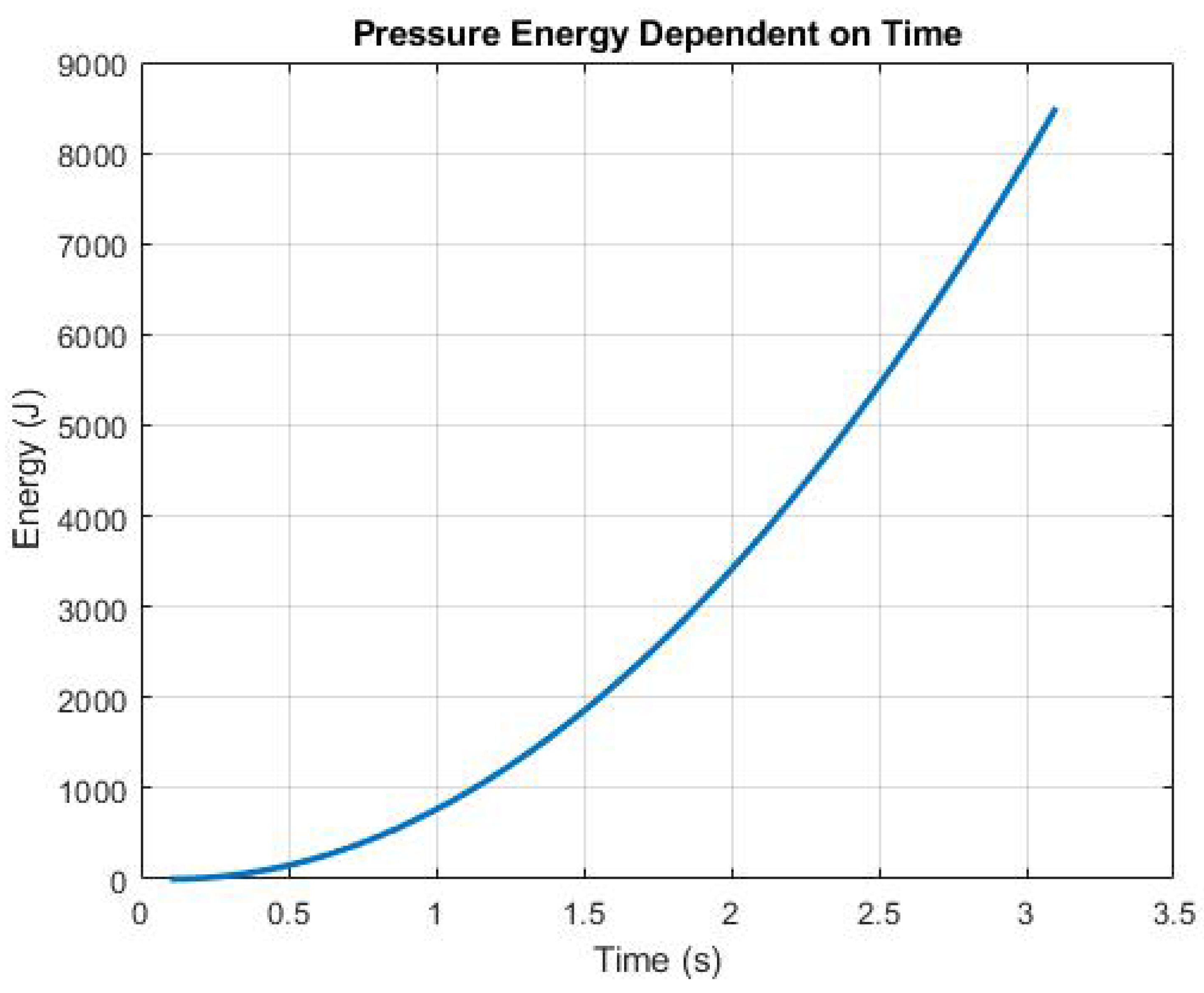
Given the linear dependency towards volumetric change, the integral presents a quadratic equation expressing the relation to the system’s energy. Analyzing the equation across a temporal interval, Figure 7 is plotted. It describes a simple parabola limited to its positive representation for the work effected, which is considered as a deformation caused by expansion.

Having a complete method to determine the energy input depending on a pneumatic source, its effects over the elastic body need to be interpreted. As hyper-elastic materials do not obey the traditional law of Hooke for linear elasticity, a different method must be employed. Several models exist with differing approximation percentages, but in this specific analysis the Neo-Hookean model was applied.

Approaching its representation through means of linear algebra, defining forces applied in three dimensions to the three basic planes of reference, a concrete approximation is given. The Neo-Hookean model considers material properties based on its proportion to the shear modulus $\mu$ and leaves deformation relations in the form of a scalar representation $I_c$.

The secondary term of the Neo-Hookean model applies only to compressible materials. The use of a strictly hyper-elastic material leads to a generalization of a universal incompressible characteristic. In any case, the Jacobian J belonging to the gradient of deformation will always equal to 1, reducing the term to 0.

The leading equation is presented.

$${\mathsf{\Psi }}_D=\frac{\mu }{2}(I_C-3)+\frac{\lambda }{2}{(J-1)}^2$$

(5)

The term $I_c$ dictates the deformation as a scalar, considering several directions and magnitudes of forces over a specific body. To determine $I_c$ the trace operation must be performed over the left Cauchy-Green deformation tensor. The square matrix denoting the Deformation Gradient, where everything is derived, is presented in a general form.

$$F_{ij}=\left[\begin{array}{ccc}{u}_x& u_y& u_z\\ v_x& v_y& v_z\\ 0& 0& {\lambda }_z\end{array}\right]$$

(6)

The general deformation gradient matrix defines three vectors describing the Euclidean planes. Each vector is associated with the directional forces. This expression is capable of describing multiple stresses indistinctly from their respective directions. Given the predictable behaviour of a soft actuator’s pneumatic chamber, a generalization can be made.

Several forces can be analyzed, but establishing a uni-axial deformation for the lateral walls of the actuator can simplify this matrix into a single diagonal dependent only on a single variable defining a relation of deformation $\lambda$ from an original length.

$$F=F^T=\left[\begin{array}{ccc}\lambda & 0& 0\\ 0& \frac{1}{\sqrt{\lambda }}& 0\\ 0& 0& \frac{1}{\sqrt{\lambda }}\end{array}\right]$$

(7)

The left Cauchy-Green deformation tensor was easily obtained by applying a matrix multiplication operation to the deformation gradient. Because the simplified matrix is only defined as a diagonal matrix, the result is the square of each individual component. Applying the trace operation; $I_c$ is the sum of the diagonal’s values.

The resolution for $I_c$ using the uni-axial deformation consideration is given in the following expression.

$$I_c=tr\left(F{F}^T\right)={\lambda }^2+\frac{2}{\lambda }$$

(8)

Substituting the new definition for $I_c$, an expression for energy through a dependent variable denoting deformation, is given. The equation can be rewritten as a cubic formula where the most prominent variable is the relation of deformation $\lambda$. The variable for energy was substituted by a conventional W to portray its relation to the initially calculated input energy.

$${\lambda }^3-\left(\frac{2W}{\mu }+3\right)\lambda +2=0$$

(9)

The solution for this equation is obtained by applying Cardano’s method for cubic equations. The main condition before using Cardano’s method is the existence of a depressed cubic equation which is already present. For problems denoting only one or two real answers, the main formula can be applied directly; however, when confronted with an equation with three interception points, the discriminants of the square roots within the method are negative. To solve this problem, the imaginary part of each segment must be expressed directly, and each term is represented as a vector containing both imaginary and real parts. To simplify further expressions, two transition variables are introduced.

The transitory term T portrays the section of Cardano’s method within a square root but is multiplied by −1 as the imaginary term i is extracted from the root. This serves as a basis to calculate the magnitudes and angles for imaginary vectors. The angle portraying the imaginary vector $\varphi$ is determined through the previously stated term T and a constant −1 found through the parameters of the initial cubic equation and those found in Cardano’s method. Because the arcsin function does not discern between which value is negative, a shift of 180 degrees is necessary to calculate the true angle, which is always expected to be in the second quadrant.

$$T=\sqrt{-1-\frac{{\left(-\left(\frac{2W}{\mu }+3\right)\right)}^3}{27}}$$

(10)

$$\varphi =180+ta{n}^{-1}\left(\frac{T}{-1}\right)$$

(11)

Each vector is separated into its components through trigonometric functions multiplied by its calculated magnitude. In view of the fact that a cubic root is still applied, the magnitude is affected directly through a radical function and the argument of the trigonometric functions is simply divided by three.

Owing to the composition of the initial formula, after applying a cubic root to both vectors, their sum is in the form of conjugates; thus, all the imaginary parts are eliminated. The remaining terms are equivalent in view of the fact that square exponents are used in the calculation of magnitude simplifying the expression further. The resolution is presented.

$$\lambda =2\sqrt[3]{\sqrt{{(-1)}^2+T^2}}\left(cos\left(\frac{\varphi }{3}\right)\right)$$

(12)

3.3. Calculation of Displacement Caused by Geometrical Changes

Referring to multi-chamber pneumatic soft actuators, the main principle of motion is a physical push between the inflated chambers. Deformation of material and restriction at base sections, creates the need for flexion between segments. Considering previous calculations for material behavior, and the geometric composition of the actuator the displacement of its parts is easily associated.

Having a solution for the relation of deformation from the initial measurement of chamber height, an approximation of deformation was used. As the material elongates owing to the inner pressure, the lateral walls form an ellipsoidal shape centered on a critical point defined as the thinnest section of the wall. If the wall states a uniformly shaped figure, the critical points form at its midpoint.

The characteristic shape of the inflated walls is that of an ellipse; thus, Euler’s base approximation for an ellipse’s perimeter P is used.

$$P=2\pi \sqrt{\frac{R_1^2+R_2^2}{2}}$$

(13)

Taking into account the fact that the height of the chambers L should remain constant thanks to the limitations of frontal and rear walls, one of the radii is taken as half the initial height. The other radius is called a lateral deformation h, relating directly to the variable circumference dependent on twice the initial length multiplied by the relation of deformation $\lambda$ previously calculated. The inverse equation is shown with an error difference from the initial value taken into account for its an approximation.

$$h=\sqrt{2{\left(\frac{2\lambda L_o}{2\pi }\right)}^2-{\left(\frac{L_o}{2}\right)}^2}-\sqrt{2{\left(\frac{L_o}{\pi }\right)}^2-{\left(\frac{L_o}{2}\right)}^2}$$

(14)

Following the studies of J. Wang [30] in a model for the behavior of a soft actuator, the formula of flexion for each segment is given. This equation depends on several design parameters such as the segment distancing c and critical deformation point b. The equation takes the lateral deformations as a dependent variable and the flexion angle as its independent variable.

$$h=\frac{b}{2cos\theta }\left(sin\theta +\frac{c}{b}+\sqrt{\frac{2c}{b}sin\theta +\frac{c^2}{b^2}}\right)$$

(15)

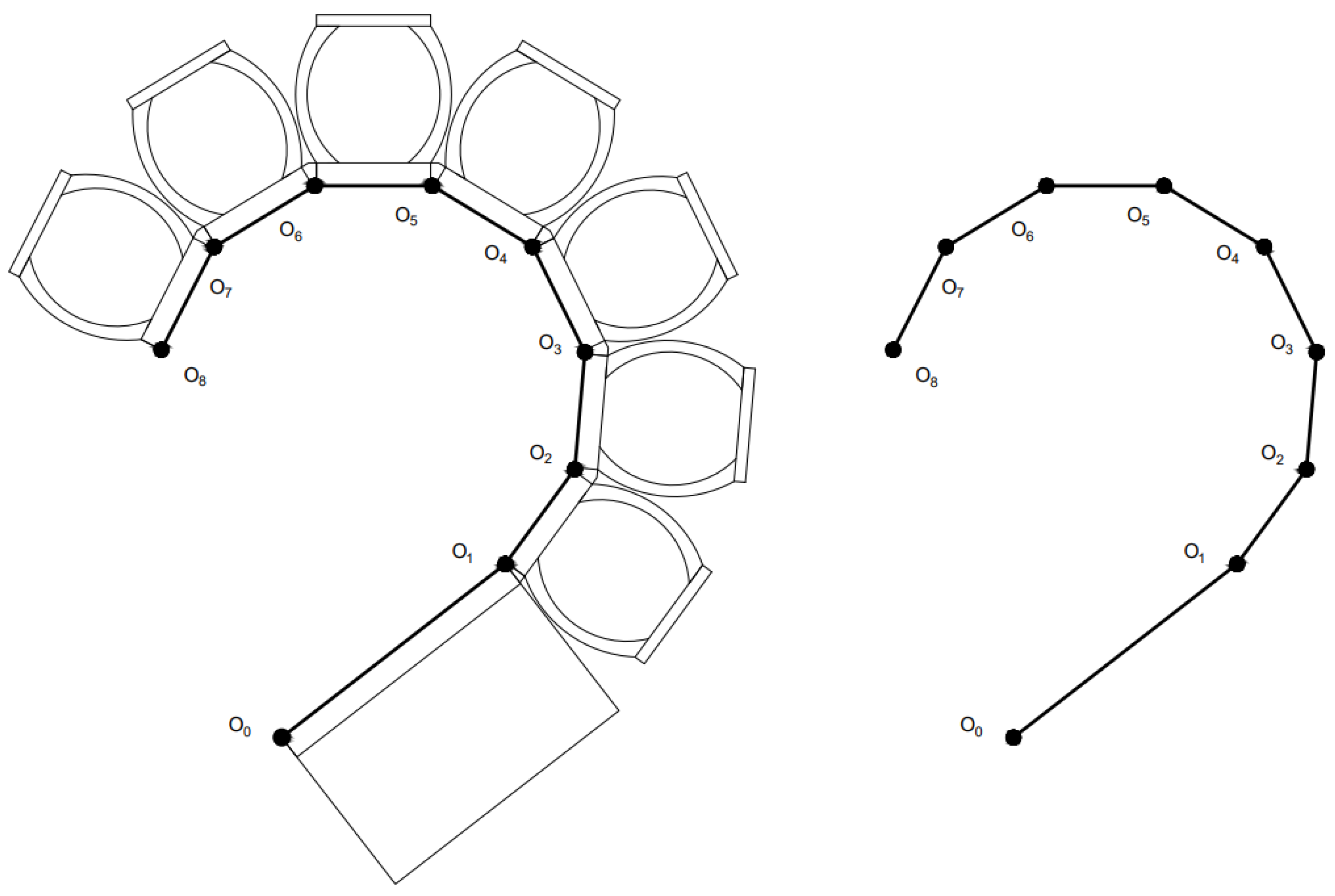
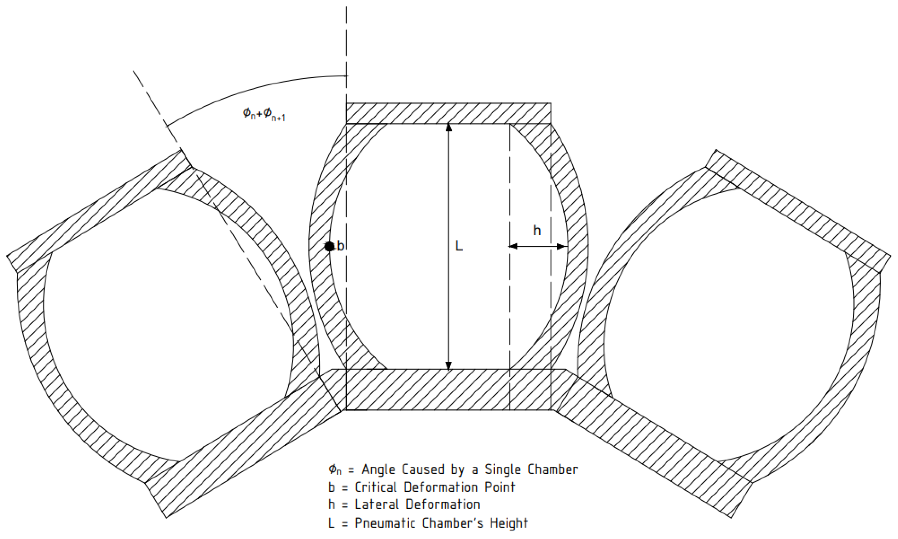
Figure 8 provides a graphic representation of the physical placements and definitions of each parameters used in the calculation of lateral deformations for individual chambers. Each chamber’s inner height is labeled as L, and h represents the lateral deformation or distance between the inner wall’s initial and situational position. The method used considers each wall’s effect separately to account for designs with variable geometries, and the complete flexion of a segment is given by the sum of its calculated angles.

Unfortunately, this takes the opposite approach to the objective of this study; therefore, an inverse function is necessary. By means of trigonometric identities and simple algebra, the result is that of a quartic equation dependent on $sin\theta$. Each coefficient is presented individually in the purpose of order.

$$A{y}^4+B{y}^3+C{y}^2+Dy+E=0$$

(16)

$$y=sin\theta$$

(17)

$$A={(b^2-4h^2)}^2+16b^2{h}^2$$

(18)

$$B=32cb{h}^2$$

(19)

$$C=16{\left(ch\right)}^2-16b^2{h}^2+8h^2(b^2-4h^2)$$

(20)

$$D=-32cb{h}^2$$

(21)

$$E=16h^4-16{\left(ch\right)}^2$$

(22)

To solve the equation, Ferrari’s method is applied, but its condition for use on depressed quartic equations is not fulfilled; therefore, variable substitution takes place in an effort to eliminate the coefficient corresponding to $y^3$.

$$y=x-\frac{B}{4A}$$

(23)

After simplifying, the new equation is presented divided into its individual coefficients, once again as a way to preserve order.

$$x^4+p{x}^2+qx+r=0$$

(24)

$$p=\frac{B^2}{8A^2}+\frac{C}{A}-\frac{B^2}{2A^2}$$

(25)

$$q=\frac{B^3}{8A^3}-\frac{CB}{2A^2}+\frac{D}{A}$$

(26)

$$r=\frac{B^4}{256A^4}-\frac{B^4}{64A^4}+\frac{C{B}^2}{16A^3}-\frac{DB}{4A^2}+\frac{E}{A}$$

(27)

Once the equation is ready, Ferrari’s method presents several transitional parameters to obtain the final result. The first parameter $\alpha$ is determined using the previously determined cubic formula. Congruence with this function ensures the applicability of further expressions.

$$q^2-8\alpha \left({\alpha }^2+p\alpha +\frac{p^2}{4}-r\right)=0$$

(28)

Cardano’s method is once again the tool of preference for a cubic equation resolution, but the necessity of a depressed cubic equation brings the need for another variable substitution.

$$\alpha =\beta -\frac{p}{3}$$

(29)

The final depressed cubic equation, which is now dependent on the variable $\beta$ is presented.

$${\beta }^3+\beta \frac{\left(-\frac{8p^2}{9}-\frac{16p^2}{9}+\frac{16p^2}{3}-2p^2+8r\right)}{-8}+\frac{\frac{2p^3}{3}-\frac{8pr}{3}+q^2-\frac{8p^3}{9}+\frac{8p^3}{27}}{-8}=0$$

(30)

Similar transition variables for Cardano’s method were employed to proceed in an orderly manner. Specifically, a term is used as a component in a vector for imaginary–real representation $Q_2$, and the angle between these components ${\varphi }_2$. The newly introduced terms $p_2$ and $q_2$ refer to the linear and independent coefficients of the previous equation, respectively.

Contrary to the obligatory use of these terms in previous implementations, they will only be used situationally when required.

$$Q_2=\sqrt{-\frac{q_2^2}{4}-\frac{p_2^3}{27}}$$

(31)

$${\varphi }_2=ta{n}^{-1}\left(\frac{Q_2}{\left(-\frac{q_2}{2}\right)}\right)$$

(32)

Faced with uncertainty about the sign of the discriminant derived by the variation of possible combinations of variables, the necessity for a piece-wise equation is clear. Both the classic solution and the answer, achieved through a detour into complex mathematics, are stated dependent on the sign of the discriminant. The solution for $\beta$ and thus a direct relation to $\alpha$ is achieved, where ${\alpha }_o$ will be a real answer to the initial equation. Even while all limits within the function exist, it fails in its continuity because there exists a point where it lacks a derivative where the boundary between domains lies.

$$\beta =\left\{\begin{array}{c}\sqrt[3]{-\frac{q_2^2}{4}+\sqrt{\frac{q_2^2}{4}+\frac{p_2^3}{27}}}+\sqrt[3]{-\frac{q_2}{2}-\sqrt{\frac{q_2^2}{4}+\frac{p_2^3}{27}}};\frac{q_2^2}{4}+\frac{p_2^3}{27}>=0\hfill \\ 2\sqrt[3]{\sqrt{{\left(-\frac{q_2}{2}\right)}^2{T}_2^2}}\left(cos\frac{{\varphi }_2}{3}\right);\frac{q_2^2}{4}+\frac{p_2^3}{27}<0\hfill \end{array}\right.$$

(33)

After obtaining the variable ${\alpha }_o$, the secondary transition parameter to be resolved is $x_o$ which correlates directly.

$$x_o=\frac{q_2}{4{\alpha }_o}$$

(34)

The value of ${\alpha }_o$ must be chosen carefully so that the resulting secondary parameter permits a real answer, because of the use of square roots for the final solution of the initial quartic equation.

$$x_n=\frac{\pm \sqrt{2{\alpha }_o}\pm \sqrt{2{\alpha }_o-4(-x_o\sqrt{2{\alpha }_o}+\frac{p_2}{2}+{\alpha }_o)}}{2}$$

(35)

Using the previously stated substitution and the arcsin trigonometric function, a method is acquired to obtain the flexion of each segment of a soft actuator depending on its input pressure.

The graph presented in Figure 9 shows a behavior granted by two radical equations with a clear inflection point. This is caused by the use of a piece-wise function to finalize the resolution of the quartic equation. Idealizing the system, the graph presents a steep continuous radical form, making this a close approximation with a small zone of poor effectiveness. The eventual curvature of the graph proves how the tension accumulated within the body of the actuator gradually prevents further displacement.

3.4. Angular Representation Using Linear Vectors

The representation of the actuator’s backbone curve is approached through a series of linear vectors $Z_n$ established in succession, depicting the magnitude and direction of each segment in concordance with the initial reference state. Each vector is composed of magnitude corresponding to segment length $L_n$ and its global angle ${\Theta }_n$ dependent on both half angles ${\theta }_n$ caused by adjacent pneumatic chambers.

$$Z_n=(L_n,{\Theta }_n)$$

(36)

The use of linear vectors is justified by the lack of change in particular segments accomplished by using conventional designs. The axis of rotation defined for each chamber was located at a midpoint of their length in separation. The design was further adjusted to this assumption, for it is the thinnest part of the body in a radial direction to the center point of its flexion. Because a requirement for the backbone curve is that its tangential vectors are always orthogonal to the transverse area and given that the base of the actuator will not suffer from longitudinal deformations, it was selected as the reference as shown in Figure 10. Areas such as the top or center of inertia show troublesome results, because their magnitude is variable in view of the fact that they contain actively deforming parts or separating pieces.

Owing to the dependence of a previous segment to determine the position of the next one, the use of recursive equations is evident. The angles expressed beforehand are relative only to the study of individual chambers and thus must be introduced to a representation of the system as a whole. To calculate a global angle $\Theta$ from the initial reference, the previous iteration of global angle is to be summed to the effects of both half angles.

$${\Theta }_n={\Theta }_{n-1}+{\theta }_n+{\theta }_{n-1}$$

(37)

Once the direction and magnitude are obtained through design parameters such as segment length $L_n$, the remaining matter is the resolution of the origin points $O_n$ for each vector. It comes naturally through another recursive equation dependent on the components of the previous origin point summed with the components of the last vector calculated using simple trigonometric functions.

$$O_n(x,y)=O_{n-1}(x,y)+(L_{n-1}cos\left({\Theta }_{n-1}\right),L_{n-1}sin\left({\Theta }_{n-1}\right))$$

(38)

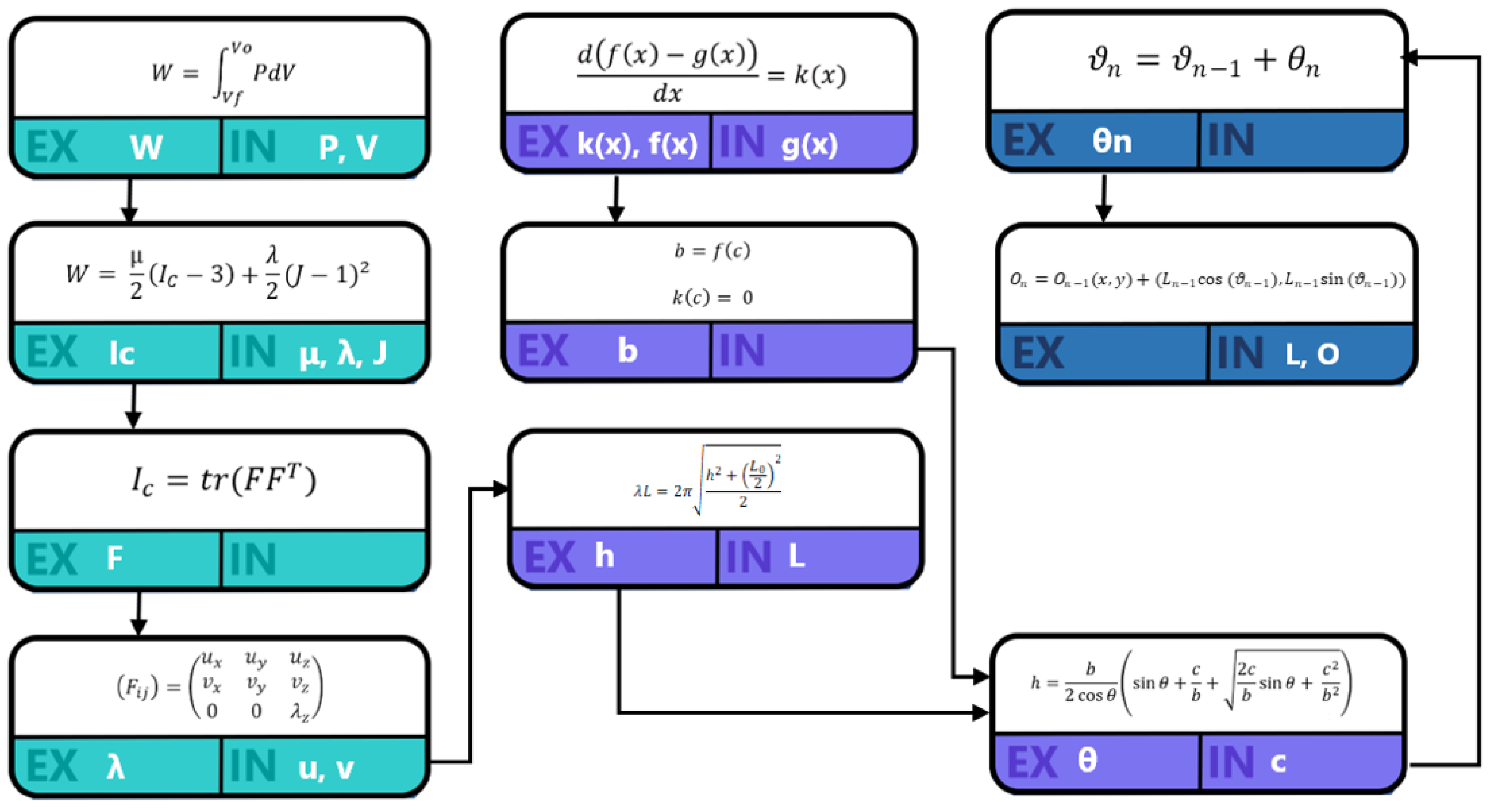
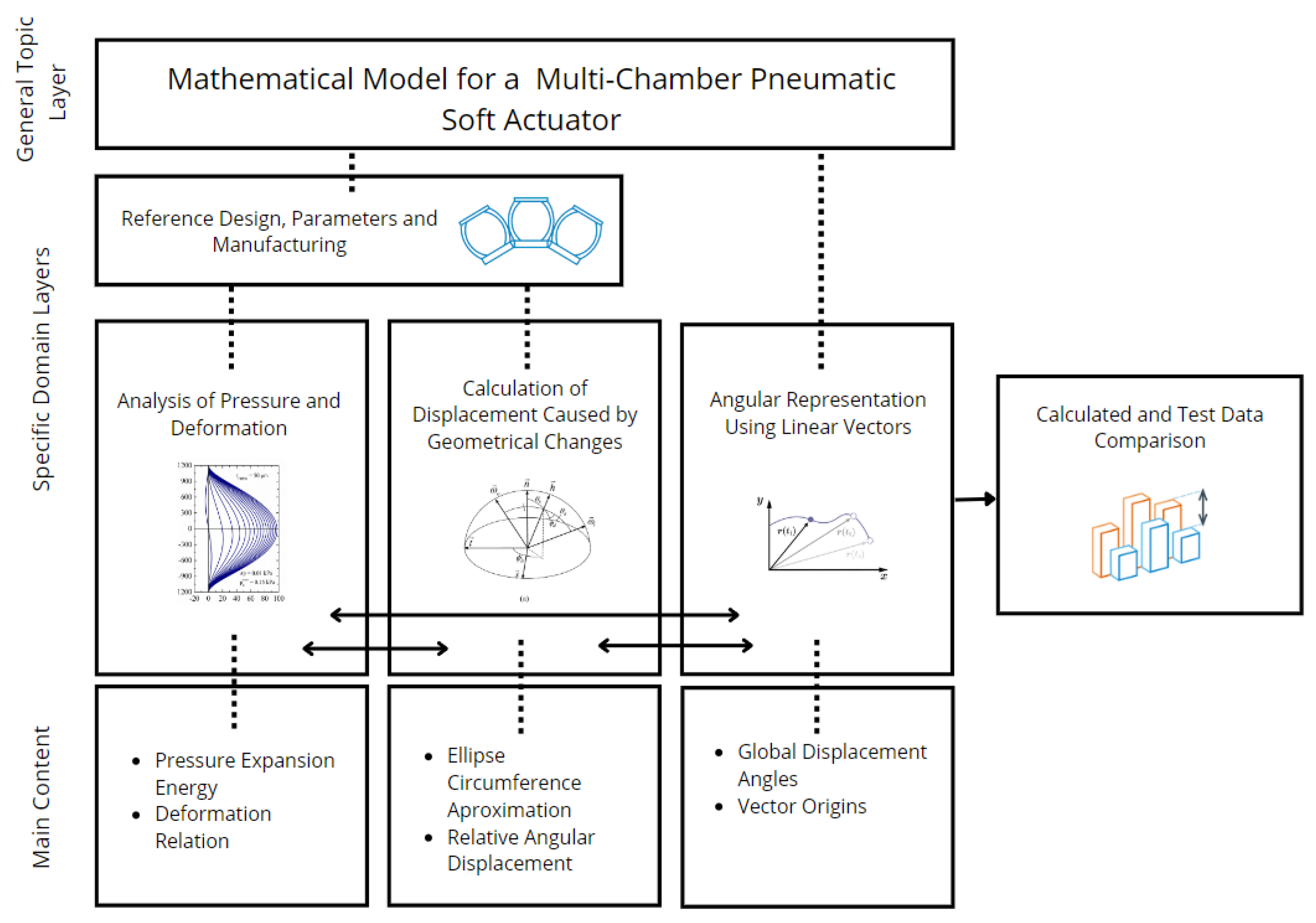
The connection of origin coordinates represent the backbone curve of the soft actuator located at its base in any given state dictated by the input pressure from the air flow source. The complete mathematical model can be summarized in Figure 11 where the principal equations on their base form are presented and classified into their corresponding domain of analysis. The colors cyan, purple and blue correspond to the analysis of pressure, deformation and the calculation of displacement caused by geometrical changes and angular representation using linear vectors sections, respectively. The model starts from the energy source and finalizes on a vectorial representation, granting graphic results.

3.5. Calculated and Test Data Comparison

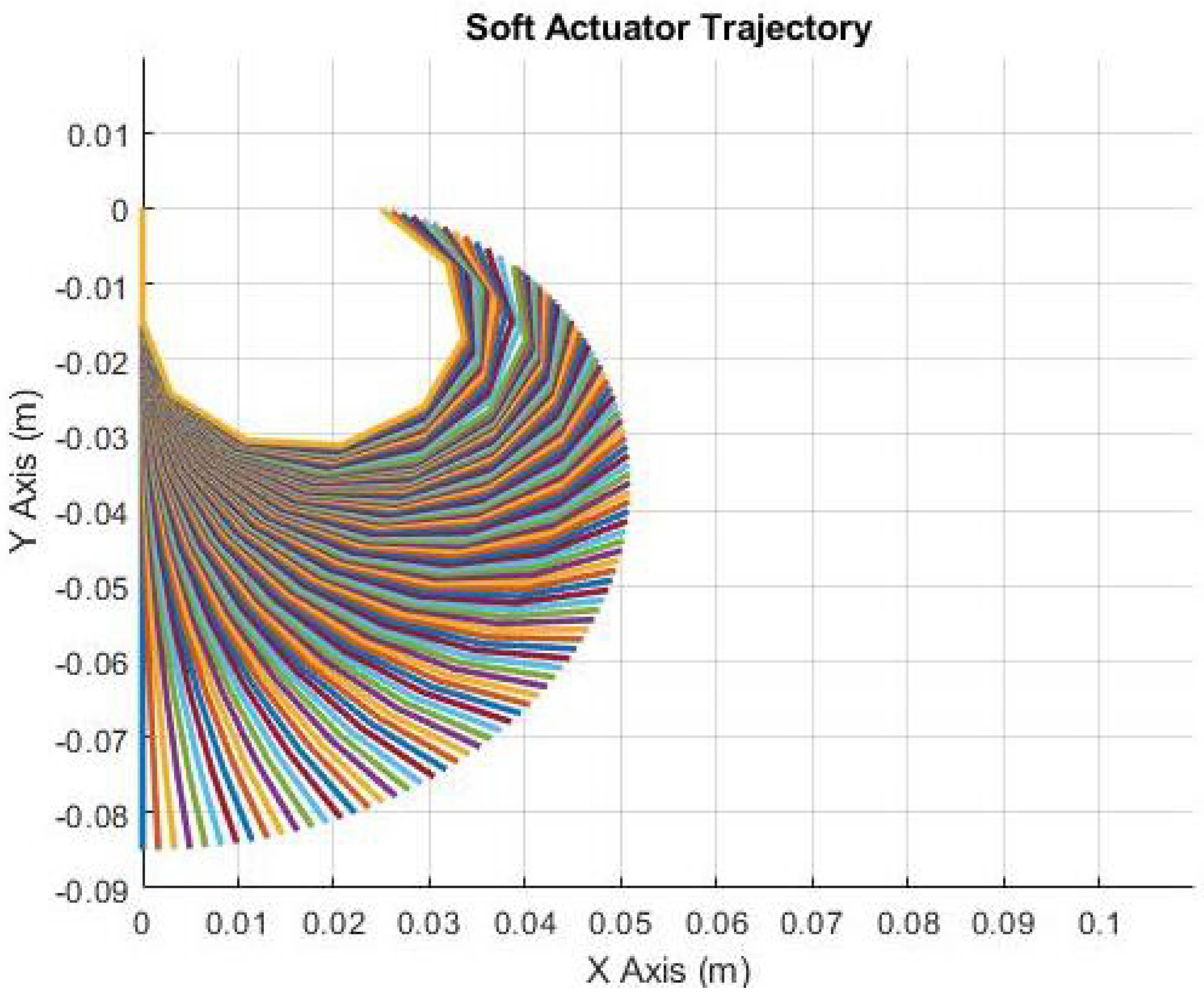
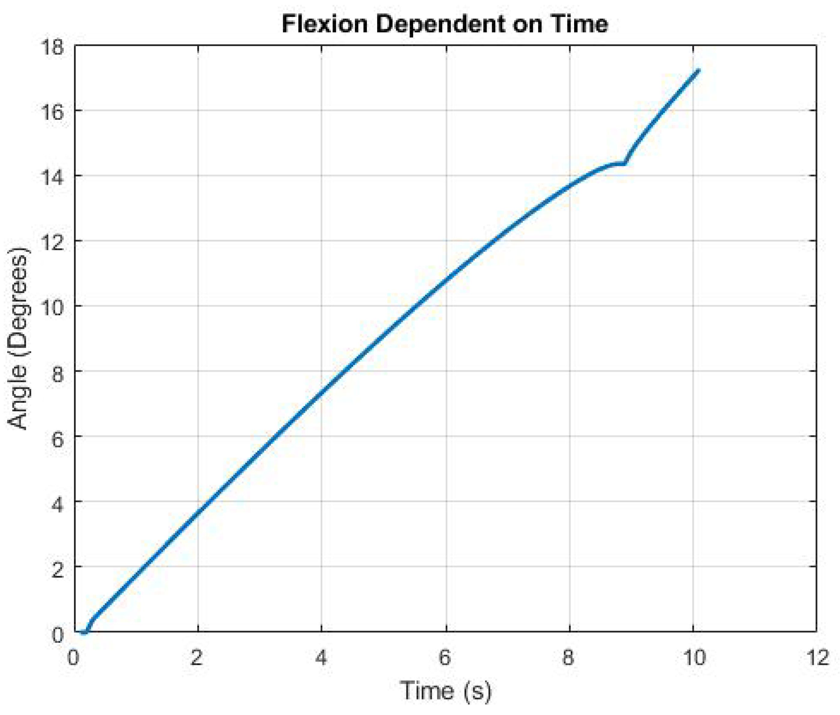
As time passes, the internal volume increases and the segment angles become more pronounced. Figure 12 presents different positions separated by 0.1 s in time. Even though each result is given at a uniformly spaced interval, it is clear that the initial plots are more physically separated. Later graphs are almost presented superimposed over each other. Although the energy source adapts to satisfy a constant volumetric flow, the flexion of the actuator depends on the ellipsoidal interaction between the chambers. At higher lateral deformations, less of the actual segments will be in contact, thus slowing its angular velocity.

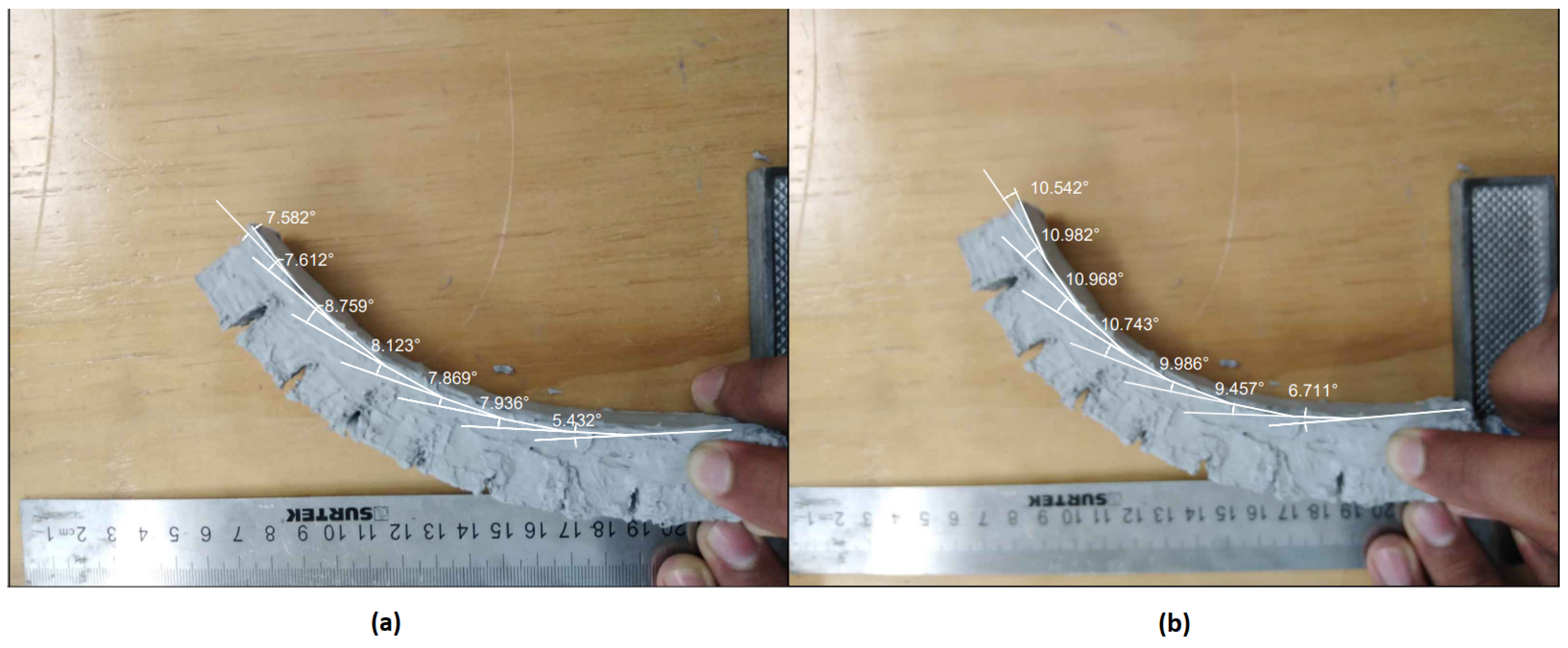
To validate results, various empirical samples were taken about the body of the actuator under different conditions. Body flexion of was controlled and measured using a pressure regulator with an integrated manometer. Photographs were obtained from a lateral view at pressures of 0.5, 1.0, 1.5, and 2.0 kg/cm². Figure 13 presents the results at 1.5 and 2.0 kg/cm² and its angle measurements taken per chamber relative to the corresponding previous segment.

The major limitation encountered in this study was the supply of compressed air. This did not allow validation with angles greater than those shown in the results. As future work, the model should be tested with other materials that have greater deformation to validate larger angles.

Relying on the relationship between pressure and volumetric deformation, the exact time expressed by the model can be calculated by applying calculations at a specific pressure. Such methods were used to create comparisons with real calculations. Figure 14 present graphic representation of the backbone curve of a soft actuator set at 1.5 and 2.0 kg/cm² using the geometrical parameters designed for the real test prototype.

The reference taken was the initial position of the first segment which was considered to be constant. The backbone curve was drawn by tracing the inflection points between segments.The slight difference in measurement is due to the composition of the material as well as human errors in prototype manufacturing. The first angle is notoriously smaller because the flexion at that particular point is dependent only on one active segment as the initial constant segment lacks a pneumatic chamber to contribute towards the flexion of the actuator.

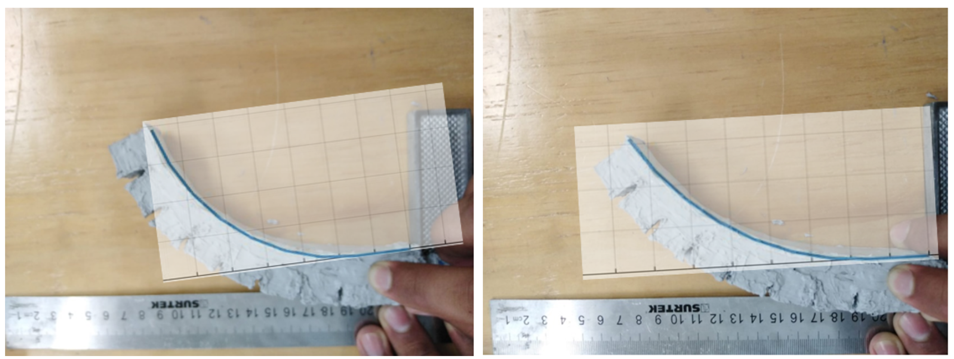
A comparison between test photographs and the modeled backbone curve is presented in Figure 15 with a superposition between images. The angle of the graphed model shifts to correlate with the reference line which is the initial segment.

The contents listed in

Table 1. Comparison between measured angles and mathematical model’s results (Radians).

kg/cm2	kPa	${\mathit{\theta }}_1$1	${\mathit{\theta }}_2$	${\mathit{\theta }}_3$	${\mathit{\theta }}_4$	${\mathit{\theta }}_5$	${\mathit{\theta }}_6$	${\mathit{\theta }}_7$	${\mathit{\theta }}_{\mathbf{Avg}}$	Model	Error
0.5	49.03	0.0339	0.0597	0.0561	0.0524	0.0514	0.0541	0.0617	0.0555	0.0462	0.0096
1	98.07	0.0520	0.085	0.083	0.085	0.087	0.074	0.072	0.080	0.0921	−0.011
1.5	147.1	0.094	0.138	0.137	0.142	0.153	0.133	0.132	0.139	0.137	0.0016
2	196.1	0.117	0.165	0.174	0.187	0.191	0.192	0.184	0.182	0.182	−0.0001

¹ θ₁ is not taken into consideration when calculating the average.

provide the individual results for the angular displacement for each segment at the four pressure conditions mentioned. To compare test results with the calculated predictions, an average value was obtained from the angles ${\theta }_2-{\theta }_7$. This approach was permitted due to the fact that all chambers were designed with equivalent geometries. Angle ${\theta }_1$ is omitted because its movement depends only on a single active chamber, this being a different instance from that of the rest of the segments.

The results are provided in degrees in

Table 2. Comparison between measured angles and mathematical model’s results (Degrees).

kg/cm2	kPa	${\mathit{\theta }}_1$1	${\mathit{\theta }}_2$	${\mathit{\theta }}_3$	${\mathit{\theta }}_4$	${\mathit{\theta }}_5$	${\mathit{\theta }}_6$	${\mathit{\theta }}_7$	${\mathit{\theta }}_{\mathbf{Avg}}$	Model	Error
0.5	49.03	1.949	3.425	3.215	3.005	2.945	3.104	3.538	3.205	2.654	0.551
1	98.07	2.983	4.875	4.762	4.870	4.967	4.231	4.123	4.638	5.285	−0.647
1.5	147.1	5.432	7.936	7.869	8.123	8.759	7.612	7.582	7.980	7.888	0.091
2	196.1	6.711	9.457	9.986	10.743	10.968	10.982	10.542	10.446	10.456	−0.009

¹ θ₁ is not taken into consideration when calculating the average.

to facilitate the understanding of the magnitudes presented.

Comparing the average with the theoretical results, the maximum error was that of 0.647° at a pressure of 1 kg/cm². The model grants precision at elevated deformations. This is attributed to the fact that the ellipsoidal geometrical approximation is advised only for ellipses with radii that do not differ significantly in magnitude. This holds true, as tests with low deformation are less precise.

4. Discussion

The results validate that at high deformations, which reflect concrete and applicable states for industrial and experimental use, a simple deterministic model is accurate at predicting the position and trajectory of multi-chamber pneumatic soft actuators. A notable increase in error can be encountered at the initial positions but the modeled values are sufficient, especially taking into account the fact that these transitory positions are rarely used as a practical end point. Even though the error was significantly reduced, the quantity of pneumatic chambers considered affects the error to the total sum of angles referring to the final angular displacement of the actuator´s tip from the reference point.

The finalized model is mainly intended for use with a constant air flow provided by a controllable source such as an air compressor or an air pressure pipeline coupled with an appropriate pneumatic pressure regulation system. This provides a clear way to create a time-dependent system for further analysis of its variables. Since pressure, volume and time are closely related to the first steps into energy calculation, a direct relationship can be formulated to determine the pressure of the system at any given time, which is how the specific model values where acquired.

The relative angles $\theta$ are not easily represented physically given that they do not present complete movement of any given part of the actuator but the effects of a single wall belonging to one of the two possible active pneumatic chambers. The complete angle of a segment relative to the position of the previous one can be recognized as the sum between the two walls creating flexion ${\theta }_{n-1}+{\theta }_n$. An easily interpreted result is that of the global angle $\Theta$, which represents the segment angle relative to the initial position reference.

Trajectory analysis at multiple instances in time reveal a deceleration on its angular velocity, for its displacement diminishes as the angle becomes more pronounced. Individual angles also displayed their dependency on both adjacent segments for the initial rotation axis, which always presents a smaller angle because segment $Z_o$ lacks a pneumatic chamber. This results are also seen on test measurements of a real actuator.

Several models use complex relations to provide a detailed response like that presented by J. Wang [30]. His work was used as the basis for the angular displacement analysis presented in this study, but redefined using the opposite approach. This type of analysis is usually limited to accounting for phenomena belonging directly to the actuator’s body, generalizing any type of external influence. The addition of an energy source interpretation creates a direct relation to the full purpose of the actuator in its entirety.

Other models for multi-chamber soft actuators were created by adopting dynamic approaches to movement [4,20]. This provides a precise analysis of their movement at the cost of simplicity, for equations become increasingly complex and difficult to adapt. The model presented in this research permits the study of various general variables given its ease of manipulating parameters, while accomplishing its main purpose. For the study of specific parts of the system, a different model is beneficial.

This study finalizes with the graphical representation of a backbone curve similar to other studies. This is a varied topic, for a range of methods, such as trigonometric functions, can be used to describe its behavior [15,21]. The approach used in this research, as well as that preferred for geometrically limited design models, is that of multiple recursively dependent linear vectors.

Defining the concept of instabilities as an issue with elastic structure continuously exposed to high pressures and consequential deformations, instabilities present a displacement in state without an input change occurring [31]. Considering that this model is inclined towards the industrial use of soft actuators for production chain robots, high pressures and thus deformations are not to be expected. This is true only for a design with relatively wide walls. The model’s purpose is to serve as a tool to design and innovate with future research throughout the field and thus it is encouraged to experiment with new ideas. Such an approach can be taken where instabilities are embraced as a tool to reduce energy inputs and yet achieve high deformations to achieve a certain task [32]. Although this particular model does not take instabilities into consideration, it is valuable research portraying new forms of actuation in a rapidly expanding field.

Even though it is taken as a system failure in most cases, instabilities can be used as a quantifiable tool able to be deduced through mathematical means. Such work is demonstrated by [33] through their work towards harnessing snap-through instabilities as a method of optimizing energy efficiency through a reduction in their necessary input while still achieving high deformations. They present the mathematical means to deduce the deformation the material will endure and thus presents a possible addition even for a deterministic model such as the one presented in this study. This would be an addition towards the complexity of the Neo-Hookean model for nonlinear elastic deformations, providing reliable results even in presence of instabilities.

5. Conclusions

In this study, a geometric approach was adopted towards the mathematical description of a multi-chamber pneumatic soft actuator dependent on the energy provided from air flow source. The Neo-Hookean model is used as a basis to link the traditional energy equilibrium physics to the behavior of nonlinear hyper-elastic materials comprising the body of the actuator. Taking approximations through the study of ellipses and using previous works as a basis for the geometrical compliance of multi-chamber configurations, angular displacement referent to individual segments is achieved.

The use of recursive equations presents a means of representing the actuator’s position in different states through the backbone curve. This was established in concordance with the actuator’s base providing an easily understandable graphic with constant magnitudes and an initial segment used as reference.

A specific design was created with the intent of validating the results portrayed by the mathematical model. Using a seven-chamber configuration with constant geometries within every segment containing a single passive segment the model was tested. Test results present expected outcomes where each relative angle is almost equivalent for every rotation axis with two adjacent active chambers. The first angle was always smaller because only one chamber is effecting a deformation.

A maximum error of 0.647° is observed after taking the average from the empirical results and comparing them to the model’s results. The precision of the mathematical model is sufficient for the study’s reach. At high deformations, objectively more important states, the error is mitigated considerably.

References

1. Peng, Y.; Liu, Y.; Yang, Y.; Liu, N.; Sun, Y.; Liu, Y.; Pu, H.; Xie, S.; Luo, J. Development of continuum manipulator actuated by thin McKibben pneumatic artificial muscle. Mechatronics 2019, 60, 56–65. [Google Scholar] [CrossRef]
2. Sparrman, B.; du Pasquier, C.; Thomsen, C.; Darbari, S.; Rustom, R.; Laucks, J.; Shea, K.; Tibbits, S. Printed silicone pneumatic actuators for soft robotics. Addit. Manuf. 2021, 40, 101860. [Google Scholar] [CrossRef]
3. Xu, Z.; Yao, P.; Cai, S.; Wang, Z.; Bao, G. Modeling and experimental research on bending and wrinkling of long-arm bio-soft robot. In Proceedings of the 2017 IEEE International Conference on Robotics and Biomimetics (ROBIO), Macau, China, 5–8 December 2017; pp. 842–847. [Google Scholar] [CrossRef]
4. Li, Y.; Zhou, W.; Wu, J.; Hu, G. A Dynamic Modeling Method for the Bi-Directional Pneumatic Actuator Using Dynamic Equilibrium Equation. Actuators 2021, 11, 7. [Google Scholar] [CrossRef]
5. Chen, L.; Yang, C.; Wang, H.; Branson, D.T.; Dai, J.S.; Kang, R. Design and modeling of a soft robotic surface with hyperelastic material. Mech. Mach. Theory 2018, 130, 109–122. [Google Scholar] [CrossRef]
6. Salem, M.E.M.; Wang, Q.; Wen, R.; Xiang, M. Design and Characterization of Soft Pneumatic Actuator for Universal Robot Gripper. In Proceedings of the 2018 International Conference on Control and Robots (ICCR), Hong Kong, China, 15–17 September 2018; pp. 6–10. [Google Scholar] [CrossRef]
7. Luo, J.; Jiang, P.; Li, X.; Bai, L.; Liu, F.; Chen, R. A Soft Self-Stable Actuator and Its Energy-Efficient Grasping. Actuators 2022, 11, 107. [Google Scholar] [CrossRef]
8. Suzumori, K.; Endo, S.; Kanda, T.; Kato, N.; Suzuki, H. A Bending Pneumatic Rubber Actuator Realizing Soft-bodied Manta Swimming Robot. In Proceedings of the 2007 IEEE International Conference on Robotics and Automation, Rome, Italy, 10–14 April 2007; pp. 4975–4980. [Google Scholar] [CrossRef]
9. Yu, Z.; Gao, Z.; Li, Y.; Pan, J. Closed-loop Control of a Pneumatic Soft Gripper for Fast and Accurate Response. In Proceedings of the 2020 8th International Conference on Power Electronics Systems and Applications (PESA), Hong Kong, China, 7–10 December 2020; pp. 1–5. [Google Scholar] [CrossRef]
10. Bortnikova, V.; Yevsieiev, V.; Beskorovainyi, V.; Nevliudov, I.; Botsman, I.; Maksymova, S. Structural Parameters Influence on a Soft Robotic Manipulator Finger Bend Angle Simulation. In Proceedings of the 2019 IEEE 15th International Conference on the Experience of Designing and Application of CAD Systems (CADSM), Polyana, Ukraine, 26 February–2 March 2019; pp. 35–38. [Google Scholar] [CrossRef]
11. Olander, D.R. Compression of an Ideal Gas as Classroom Example of Reversible and Irreversible Processes. Int. J. Eng. Educ. 2000, 16, 524–528. [Google Scholar]
12. Ibrahim, S.; Krause, J.C.; Raatz, A. Linear and Nonlinear Low Level Control of a Soft Pneumatic Actuator. In Proceedings of the 2019 2nd IEEE International Conference on Soft Robotics (RoboSoft), Seoul, Korea, 14–18 April 2019; pp. 434–440. [Google Scholar] [CrossRef]
13. Thuruthel, T.G.; Falotico, E.; Manti, M.; Laschi, C. Stable Open Loop Control of Soft Robotic Manipulators. IEEE Robot. Autom. Lett. 2018, 3, 1292–1298. [Google Scholar] [CrossRef]
14. Horgan, C.O. A note on a class of generalized neo-Hookean models for isotropic incompressible hyperelastic materials. Int. J. Non-Linear Mech. 2021, 129, 103665. [Google Scholar] [CrossRef]
15. Caasenbrood, B.J.; Pogromsky, A.Y.; Nijmeijer, H. Dynamic modeling of hyper-elastic soft robots using spatial curves. IFAC-PapersOnLine 2020, 53, 9238–9243. [Google Scholar] [CrossRef]
16. Smith, B.; De Goes, F.; Kim, T. Stable Neo-Hookean Flesh Simulation. ACM Trans. Graph. 2018, 37, 15. [Google Scholar] [CrossRef] [Green Version]
17. Zhao, W.; Zhang, J.; Zhang, W.; Yuan, X. Internal resonance characteristics of hyperelastic thin-walled cylindrical shells composed of Mooney–Rivlin materials. Thin-Walled Struct. 2021, 163, 107754. [Google Scholar] [CrossRef]
18. Mao, Z.; Nagaoka, T.; Yokota, S.; Kim, J.W. Soft fiber-reinforced bending finger with three chambers actuated by ECF (electro-conjugate fluid) pumps. Sens. Actuators A Phys. 2020, 310, 112034. [Google Scholar] [CrossRef]
19. Zhang, J.; Zhou, J.; Yuan, S.; Jing, C. Design, Fabrication and Experiments of a 3D-motion Soft Elastomer Actuator. In Proceedings of the 2019 IEEE International Conference on Mechatronics and Automation (ICMA), Tianjin, China, 4–7 August 2019; pp. 497–501. [Google Scholar] [CrossRef]
20. Gharavi, L.; Zareinejad, M.; Ohadi, A. Dynamic Finite-Element analysis of a soft bending actuator. Mechatronics 2022. [Google Scholar] [CrossRef]
21. Venkiteswaran, V.K.; Sikorski, J.; Misra, S. Shape and contact force estimation of continuum manipulators using pseudo rigid body models. Mech. Mach. Theory 2019, 139, 34–45. [Google Scholar] [CrossRef]
22. Mochiyama, H. The Elastic Rod Approach toward System Theory for Soft Robotics. IFAC-PapersOnLine 2020, 53, 9175–9180. [Google Scholar] [CrossRef]
23. Enojas, M.J.B.; Ramos, M.C. Development of a Finger Soft Pneumatic Bending Actuator. In Proceedings of the 2019 4th Asia-Pacific Conference on Intelligent Robot Systems (ACIRS), Nagoya, Japan, 13–15 July 2019; pp. 1–5. [Google Scholar] [CrossRef]
24. Rad, C.; Hancu, O.; Lapusan, C. Data-Driven Kinematic Model of PneuNets Bending Actuators for Soft Grasping Tasks. Actuators 2022, 11, 58. [Google Scholar] [CrossRef]
25. Kokubu, S.; Yu, W. Developing a hybrid soft mechanism for assisting individualized flexion and extension of finger joints. In Proceedings of the 2020 42nd Annual International Conference of the IEEE Engineering in Medicine & Biology Society (EMBC), Montreal, QC, Canada, 20–24 July 2020; pp. 4873–4877. [Google Scholar] [CrossRef]
26. Fras, J.; Macias, M.; Noh, Y.; Althoefer, K. Fluidical bending actuator designed for soft octopus robot tentacle. In Proceedings of the 2018 IEEE International Conference on Soft Robotics (RoboSoft), Livorno, Italy, 24–28 April 2018; pp. 253–257. [Google Scholar] [CrossRef]
27. Olson, G.; Hatton, R.L.; Adams, J.A.; Mengüç, Y. An Euler–Bernoulli beam model for soft robot arms bent through self-stress and external loads. Int. J. Solids Struct. 2020, 207, 113–131. [Google Scholar] [CrossRef]
28. Wang, T.; Lin, B.; Chong, B.; Whitman, J.; Travers, M.; Goldman, D.I.; Blekherman, G.; Choset, H. Reconstruction of Backbone Curves for Snake Robots. IEEE Robot. Autom. Lett. 2021, 6, 3264–3270. [Google Scholar] [CrossRef]
29. Hehenberger, P.; Poltschak, F.; Zeman, K.; Amrhein, W. Hierarchical design models in the mechatronic product development process of synchronous machines. Mechatronics 2010, 20, 864–875. [Google Scholar] [CrossRef]
30. Wang, J.; Fei, Y.; Pang, W. Design, Modeling, and Testing of a Soft Pneumatic Glove With Segmented PneuNets Bending Actuators. IEEE/ASME Trans. Mechatron. 2019, 24, 990–1001. [Google Scholar] [CrossRef]
31. Hrinda, G. Snap-through Instability Patterns in Truss Structures; American Institute of Aeronautics and Astronautics, NASA Langley Research Center: Hampton, VA, USA, 2010. [Google Scholar]
32. Pal, A.; Restrepo, V.; Goswami, D.; Martinez, R.V. Exploiting Mechanical Instabilities in Soft Robotics: Control, Sensing, and Actuation. Adv. Mater. 2021, 33, 2006939. [Google Scholar] [CrossRef]
33. Overvelde, J.T.B.; Kloek, T.; D’haen, J.J.A.; Bertoldi, K. Amplifying the response of soft actuators by harnessing snap-through instabilities. Proc. Natl. Acad. Sci. USA 2015, 112, 10863–10868. [Google Scholar] [CrossRef] [Green Version]
Figure 1. Research and Analysis Domain Divisions.
Actuators 11 00221 g001
Figure 2. Diagram of multi-chamber pneumatic soft actuator’s inner and outer geometry.
Actuators 11 00221 g002
Figure 3. Measurements of a soft actuator’s individual component.
Actuators 11 00221 g003
Figure 4. Two-Piece Mold for Soft Actuator Component Manufacturing.
Actuators 11 00221 g004
Figure 5. 3D-Printed Mold with Curated Hyper-elastic Material.
Actuators 11 00221 g005
Figure 6. Soft Actuator Coupled to an Industrial Robot.
Actuators 11 00221 g006
Figure 7. Energy input from pressure source defined by the constant change in volume.
Actuators 11 00221 g007
Figure 8. Physical definitions of variables in the calculation of flexion.
Actuators 11 00221 g008
Figure 9. Change in angle per chamber through constant air input.
Actuators 11 00221 g009
Figure 10. Vectorial representation of a backbone curve for a soft actuator.
Actuators 11 00221 g010
Figure 11. Mathematical Model’s Equation Flow.
Actuators 11 00221 g011
Figure 12. Instances of positions spaced as more energy is introduced to the system.
Actuators 11 00221 g012
Figure 13. Test measurements of soft actuator flexion at different pressures. (a) Tested Displacement at 1.5 kg/cm2. (b) Tested Displacement at 2 kg/cm2.
Actuators 11 00221 g013
Figure 14. Modeled Displacement of soft actuator flexion at different pressures. (a) Calculated Displacement at 1.5 kg/cm2. (b) Calculated Displacement at 2 kg/cm2.
Actuators 11 00221 g014
Figure 15. Comparison between Modeled Displacement and Test Measurements of soft actuator flexion at different pressures. (left) Comparison at 1.5 kg/cm2. (right) Comparison at 2 kg/cm2.
Actuators 11 00221 g015