Article

Autonomous Vehicle Path Planning Based on Driver Characteristics Identification and Improved Artificial Potential Field

1
College of Energy and Power Engineering, Nanjing University of Aeronautics and Astronautics, Nanjing 210016, China
2
School of Automobile and Rail Transportation, Nanjing Institute of Technology, Nanjing 211167, China
3
College of Mechanical Engineering, Yangzhou University, Yangzhou 225127, China
*
Author to whom correspondence should be addressed.
Actuators 2022, 11(2), 52; https://doi.org/10.3390/act11020052
Submission received: 15 December 2021 / Revised: 29 January 2022 / Accepted: 31 January 2022 / Published: 8 February 2022
(This article belongs to the Special Issue Intelligent Control and Robotic System in Path Planning)

Abstract

:
Different driving styles should be considered in path planning for autonomous vehicles that are travelling alongside other traditional vehicles in the same traffic scene. Based on the drivers’ characteristics and artificial potential field (APF), an improved local path planning algorithm is proposed in this paper. A large amount of driver data are collected through tests and classified by the K-means algorithm. A Keras neural network model is trained by using the above data. APF is combined with driver characteristic identification. The distances between the vehicle and obstacle are normalized. The repulsive potential field functions are designed according to different driver characteristics and road boundaries. The designed local path planning method can adapt to different surrounding manual driving vehicles. The proposed human-like decision path planning method is compared with the traditional APF planning method. Simulation tests of an individual driver and various drivers with different characteristics in overtaking scenes are carried out. The simulation results show that the curves of human-like decision-making path planning method are more reasonable than those of the traditional APF path planning method; the proposed method can carry out more effective path planning for autonomous vehicles according to the different driving styles of surrounding manual vehicles.

1. Introduction

Autonomous vehicles can drive based on the perception of surrounding environmental conditions, just like human drivers [1]. In recent years, research on autonomous driving has become a hot spot. Advanced Driving Assistant System (ADAS) has developed rapidly, and some technologies have been applied in mass production [2]. The autonomous driving system contains a wide range of technologies, including multi-sensor fusion technology, signal processing technology, communication technology and artificial intelligence technology [3]. Autonomous driving technology can be summarized as: “Identify the surrounding environment through a variety of on-board sensors, and make analysis and judgments based on the obtained environmental information, thereby controlling the movement of the vehicle, and ultimately achieving autonomous driving”.
Autonomous driving technology mainly includes three parts: perception, planning and controlling [4]. Planning is the key to autonomous driving. It is necessary to make reasonable judgments on the scene to ensure the safety of autonomous vehicles. It acts as a decision maker. On the basis of satisfying safe driving, the comfort of the vehicle must also be considered to realize different plans for different types of driving scenarios.
In order to improve the planning capabilities of automated vehicles, it is of great significance to introduce the driver models. Autonomous driving is still a long time away from large-scale commercial applications. For a long time in the future, there will be a traffic scene where autonomous vehicles and traditional vehicles coexist [5]. Therefore, autonomous vehicles must effectively identify the driver characteristics of the surrounding traditional vehicles, which allows autonomous vehicles to have more reasonable plans. As in [6], a non-cooperative vehicle-to-vehicle trajectory-planning algorithm with consideration of the characteristics of different drivers is presented. A non-cooperative control algorithm considering each of the driver–vehicle systems as a player is employed to plan collision-free trajectories for the encountering vehicles with respective initial driving intentions. The non-cooperative problem is solved with the theory of Nash equilibrium and is ultimately converted to a standard nonlinear Model Predictive Control problem. In [7], a driver detection system is developed to warn the driver of the current traffic conditions. It uses vehicle status and sensor detection signals to analyze the driver’s status, and provides a reasonable driving operation mode to enhance the driver’s operating experience.
There are three main categories of driver classification [8]: (1) detection based on head movement changes [9]; (2) detection based on the driver’s mental state [10]; (3) detection based on the driver’s handling characteristics [11]. The research carried out in this paper aimed to determine a driver’s category by detecting his/her manipulation behavior.
Based on the driving characteristics of the driver, it is necessary to collect operating data such as braking, acceleration and steering during driving. The driver will plan their route based on the state of the vehicle, the state of other vehicles and road conditions. Fixed algorithms often make inherent driving strategies for complex and changeable driving conditions, and will not have personalized decision-making methods. However, age, gender, driving experience, subjective emotions and mental states will all have different effects on the driver at a given moment [12].
As a research hotspot in autonomous driving technology, there are many algorithms in path planning, including the A* algorithm [13,14], Rapidly-exploring Random Tree (RRT) [15,16], Artificial Potential Field (APF) [17,18,19] and some other path planning methods for collision avoidance problems [20,21,22,23], et al.
The A* algorithm is a typical heuristic path planning algorithm. It is a graph search algorithm which has been widely used in various types of robots. Hart PE proposed the A* search algorithm on the basis of the Dijkstra graph search algorithm [24]. From the principle of the algorithm, the realization of the heuristic algorithm makes fast node searching possible. Its design focus is to construct the map and determine the cost function, so it is suitable for searching the space known in advance. With the increase in the map, the cost of memory and speed also increased. As in [13], a recursive path planning method is proposed, which uses the reduced state of the search space and comprehensively considers the kinematics, shape and steering space of the vehicle for path planning. In [14], a new A* algorithm based on the equal-step sampling of the vehicle kinematics model is proposed, which combines vehicle kinematics and introduces an enhanced cost function, which greatly improves the comfort of the path.
RRT is a sampling-based path planning algorithm, which is characterized by randomly extracting the configuration space or state space, and searching for connectivity in it [25,26]. This allows rapid planning in semi-structured spaces, and it is not only suitable for ordinary two-dimensional planes, but also for three-dimensional spaces. In addition, it can also take incomplete constraints into consideration (such as the maximum turning radius of the vehicle). As proposed in [15], an improved RRT-based automatic vehicle motion planner can effectively navigate in the chaotic environment of narrow passages. Additionally, in order to smooth the trajectory, a post-processing algorithm with trajectory optimization is proposed. In [16], based on the basic RRT algorithm, a “target-oriented RRT (GRRT)” algorithm is proposed, which provides an alternative method for probabilistic target bias, thereby avoiding local collisions. However, because RRT performs a random search in the solution space, the search trajectory is random and does not guarantee uniqueness and optimality. The trajectory generated by this algorithm is not continuous, which is not suitable for autonomous vehicles [27]. With the development of algorithms, improved algorithms considered from the perspective of rapidity and optimality are gradually being applied to actual control scenarios [28].
The APF method, due to its simple structure, ideal real-time performance and the ability to generate smooth paths, has been successfully applied to many vehicles and robots. APF is derived from a virtual force method proposed by Khatib [29], which designs the motion of the robot as a motion in an artificial gravitational field, planning a safe and smooth path. In [17], a method of expressing complex-shaped obstacles by calculating the potential field of a series of circular obstacles in the harmonic potential field was proposed; in [18], a new method for automatically detecting lane change in other vehicles is proposed, which can change its position according to the distribution of neighboring vehicles, and can describe general vehicle lane change by applying dynamic latent models; in [19], an improved artificial potential field (IAPF) method is proposed, which introduces the distance between the robot and the target point into the function of the original repulsive force field. By changing the original direction of the repulsive force, the trap problem caused by the local minimum is avoided.
The path planning method for obstacle avoidance is also a current research hotspot. As in [20], to enhance the capabilities of such vehicles without increasing weight or computing power, a reactive collision avoidance method based on open sectors is described. The method utilizes information from a two-dimensional laser scan of the environment and a short-term memory of past actions and can rapidly circumvent obstacles in outdoor urban/suburban environments. In [21], a new real-time obstacle avoidance method for mobile robots was developed and implemented. This method, named the vector field histogram (VFH), permits the detection of unknown obstacles and avoids collisions while simultaneously steering the mobile robot toward the target. In [22], a new concept, the Admissible Gap (AG), for reactive collision avoidance is proposed. A gap is considered admissible if it is possible to find a collision-free motion control that guides a robot through it, while respecting the vehicle constraints. On this basis, a new navigation approach was developed, achieving an outstanding performance in unknown dense environments. In [23], a path planner solution that makes it possible to autonomously explore underground mines with aerial robots (typically multicopters) is presented. The designed path planner is defined as a simple and highly computationally efficient algorithm which, by only relying on a laser imaging detection and ranging (LIDAR) sensor with simultaneous localization and mapping (SLAM) capability, permits the exploration of a set of single-level mining tunnels.
As the requirements for control performance increase, many researchers use model predictive control algorithms (MPC) [30,31,32,33] to include constraints that need to be considered in planning. For example, Gutjahr B converts the problem of vehicle lateral tracking along a reference curve into a constrained optimization problem. Based on the linear time-varying model in the backward time domain, the vehicle is controlled to drive along the optimized roads [34]. In recent years, many algorithms combining APF with MPC have been successfully applied [35,36,37]. The main idea of this type of algorithm is to use the global reference trajectory as the gravitational field, obstacles as the repulsive force field and the resultant force as the cost function of MPC from optimization, so as to obtain the least costly control variables [35].
In order to make the planned paths more in line with the actual road conditions, some researchers have integrated the driver model into the path planning algorithm to make the autonomous vehicles have human-like characteristics. In [38], a new driver model for critical maneuvering conditions is combined with a new steering strategy. The vehicle can be adjusted to accurately follow the desired path with the driver model. Additionally, the stability of the vehicle and the smoothness of the steering angle input are comprehensively considered. In [39], a path planning method for imitating the lane-changing operation of excellent drivers is proposed. The excellent driver lane-changing model is established based on the genetic algorithm (GA) and back propagation (BP) neural network trained by the data of the lane-changing tests. The proposed approach can plan out an optimized lane change path according to the vehicle condition by learning the excellent drivers’ driving routes.
Among the above path planning algorithms, APF has been widely used in path planning in many fields due to its simplicity, efficiency and wide applicability. However, it also has limitations such as the target point may not be reached, the local minimum and the fixed potential field function. In order to solve the shortcomings of APF, this paper combines it with the driver characteristic identification, giving APF the characteristics of human-like decision making. The driving characteristics of different surrounding drivers are taken into consideration in the path planning of autonomous vehicles, so that the planned path can be adapted to different surrounding manual driving vehicles.
The primary contributions of this paper lie in two aspects: (1) the driver characteristic identification algorithm based on the K-means clustering analysis algorithm and Keras neural network model can accurately classify the driving styles of different drivers; (2) an improved APF combined with driver characteristic identification is proposed. The designed local path planning method can adapt to different surrounding manual driving vehicles.
This paper is organized as follows: Section 2 introduces the driver identification test. Section 3 classifies the test data and imports them into the Keras neural network model for learning. Section 4 combines the drivers’ characteristic identification with IAPF, and proposes an improved local path planning algorithm. Section 5 presents the simulation and results of the proposed path planning paradigm in this paper. Conclusions are made in Section 6.

2. Driver Characteristic Identification

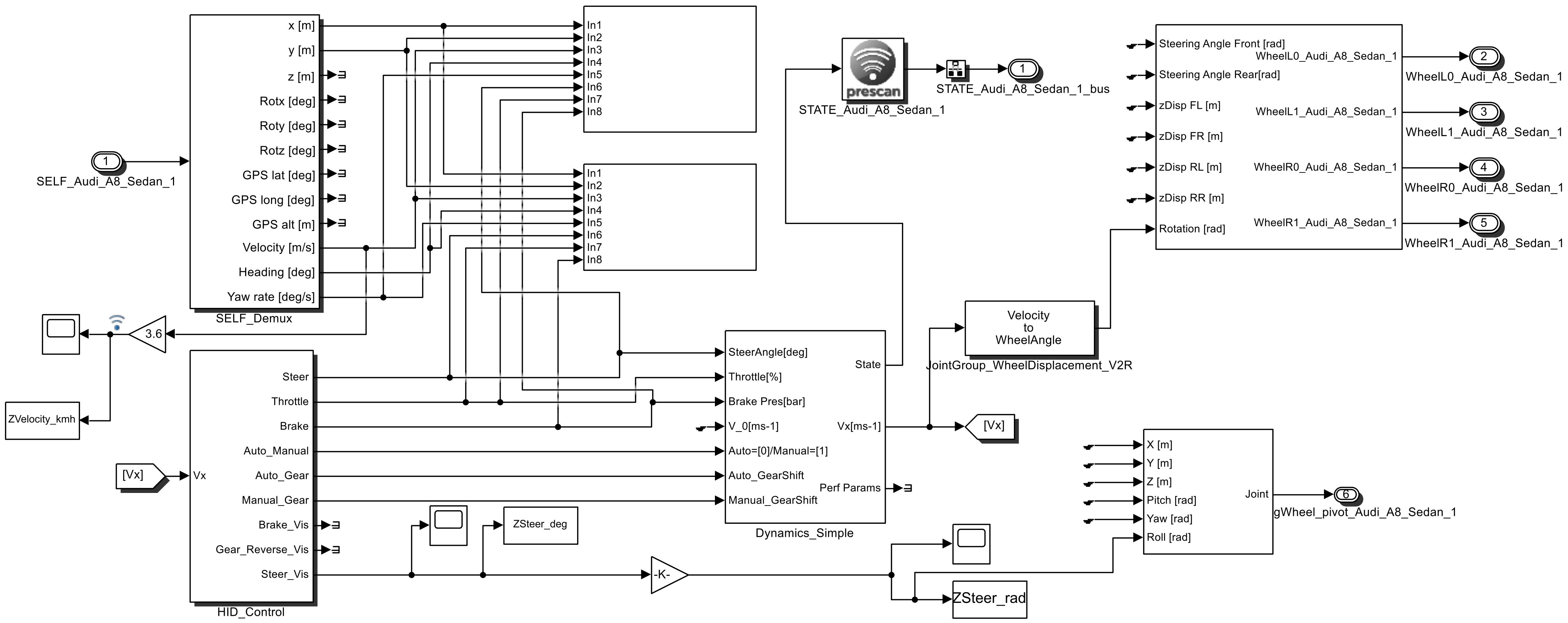
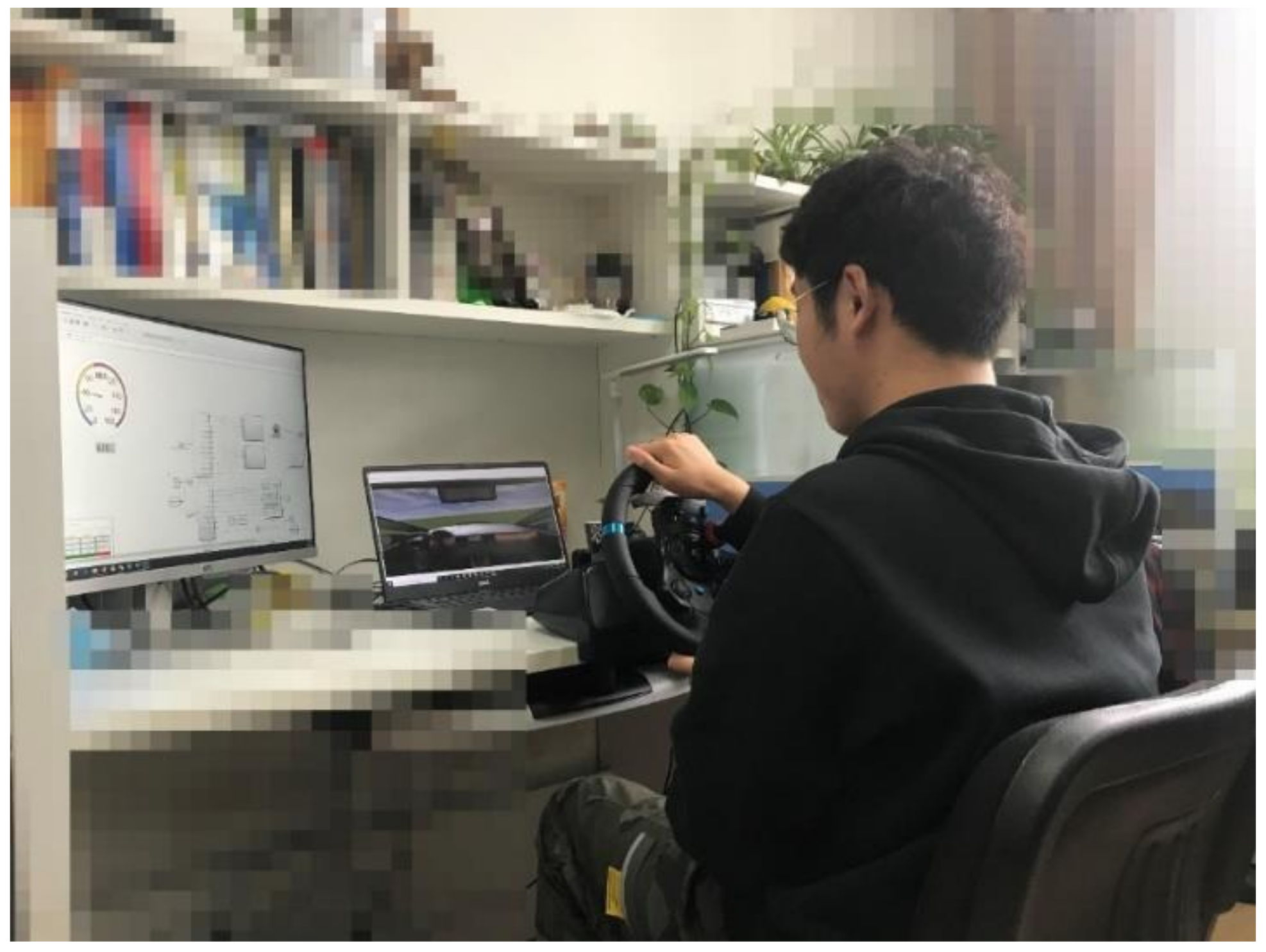
A semi-physical simulation platform was used in the test. A virtual test platform was built by Matlab/Simulink powered by MathWorks (Natick, Massachusetts 01760, USA) and Prescan powered by Siemens (80333 Munich, Germany). A driving control platform for the driver was provided by Logitech G29. The driver characteristic identification test was established to accurately reflect the differences in driving behavior of different drivers.

2.1. The Experimental Scene Construction

Studies have shown that certain objective driving factors, such as gender, age and driving experience, all have impacts on driving habits; subjective driving factors, such as emotions and traffic scenes, are the same [40]. A driver may show different characteristics in different driving scenarios. Therefore, the above conditions need to be fully considered in selecting testers. In order to distinguish the driving proficiency of the testers, they were divided into three sections in terms of driving age, namely, 0–3 years, 3–6 years and more than 6 years. There were 30 drivers of different ages, genders and driving ages in the tests. The specific statistics are shown in Table 1 and Table 2.
The virtual driving test platform was composed of Matlab/Simulink, Prescan and Logitech G29. When establishing a joint virtual driving experiment platform, it is necessary to download and install the G29 driver software on Logitech’s official website, and then install and connect the steering wheel and pedal kit to the computer. The configuration file of Prescan is created in the driver software. The button settings and sensitivity of the steering wheel, up/down gear and pedal kit are set to achieve true driving torque feedback. It is the most critical to establish the relationship between the vehicle and the G29 control model in Prescan. The specific method is to select the dynamic model in “Dynamics” in “Object Configuration”, then select “Game Controller” in “Driver Model”, select “Logitech G29” and check “Force Feedback”. Matlab/Simulink is the linker of Prescan and Logitech G29. It provides Prescan with the corresponding vehicle dynamics model and transmits the signals of G29 to Prescan. Figure 1 shows the Prescan and Matlab joint simulation platform.
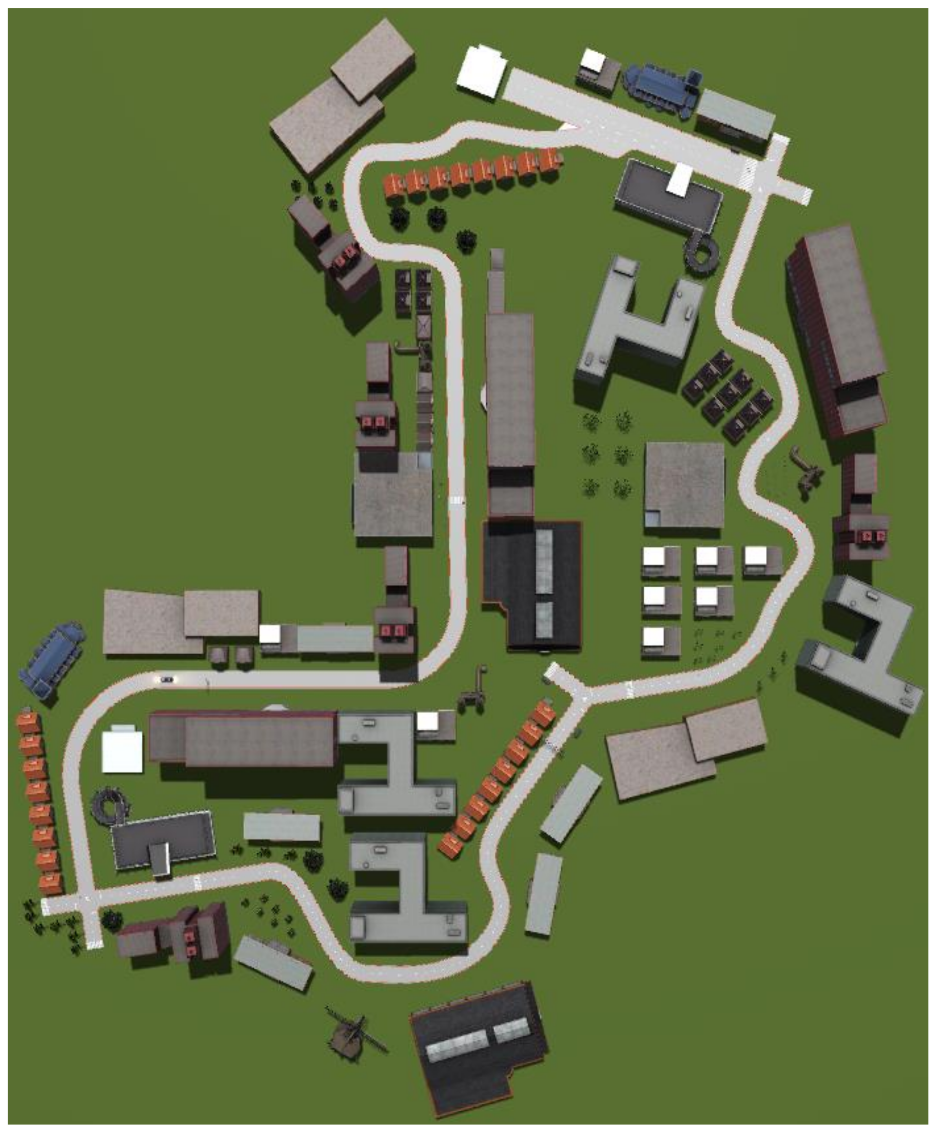
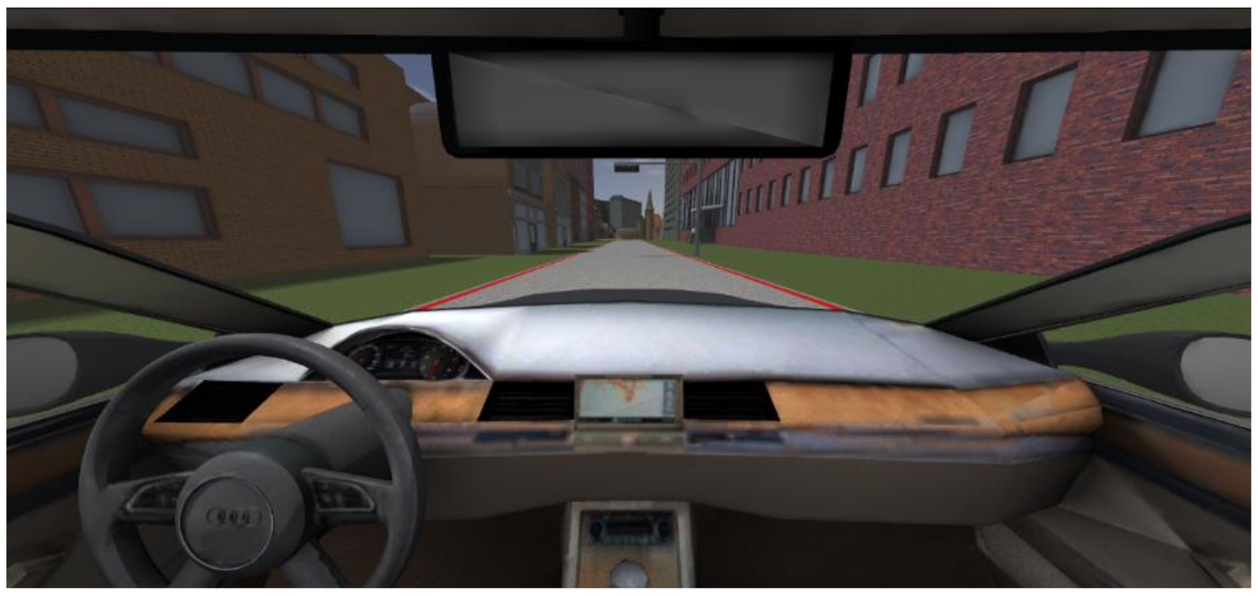
In the tests, the driving scene was the basis for distinguishing the driving characteristics of different drivers. It was built in Prescan, taking into account many factors, such as roads, signal lights, buildings and weather. The built-up driving scene is shown in Figure 2. The driver’s viewing points and driver under test are shown in Figure 3 and Figure 4.

2.2. Collection and Processing of Experimental Data

The test vehicle was set to Audi_A8_Sedan of Volkswagen, Germany. In the test, the following data of each driver were collected: driving time, t; throttle, L; brake pressure, P; steering wheel angle, δ ; speed, v; Yaw rate, γ ; vehicle heading angle, h. Braking, acceleration and steering were the drivers’ main behaviors, so the throttle, braking pressure and steering wheel angle were three important influence factors. The other three variables were affected by these three operations and served as auxiliary factors.
Data of drivers in the curve needed to be separated. The data were in the same time scale, so the steering wheel angle could be used as the criterion; when the absolute value of the steering wheel angle was less than 10° or greater than 10°, but the duration was less than 2 s, it was considered that the vehicle had no steering operation [41]. Therefore, the relevant operations during the steering process of drivers could be filtered out. Two aspects of steering wheel angle data were processed: steering wheel angular speed and steering wheel angle standard deviation; the specific formulas are as follows:
v δ = δ max δ min t max t min
σ δ = 1 n i = 1 n ( δ i δ ¯ ) 2
In Equations (1) and (2), v δ is the steering wheel angular speed, which indicates the average speed of the steering wheel during per segment steering operation time. δ max indicates the maximum steering wheel angle in this section of steering operation; δ min indicates the minimum steering wheel angle in this section of steering operation. σ δ is the standard deviation of the steering wheel angle, which represents the standard deviation of the steering wheel angle during the n-segment steering operation of the driver during per test. n is the number of steering operations extracted from the driver’s experimental data. The meaning of n in the subsequent formulas in this section is the same. δ i is steering wheel angle, and δ ¯ is the mean value of the steering wheel angles.
The processing methods of throttle and brake pressure were similar to those of the steering wheel angle. The contents of the throttle were the changing rates and the standard deviation of the throttle. The contents of the brake pressure data processing were the average and the standard deviation of the braking pressure. The specific formulas are as follows:
L = L max L min t max t min
δ L = 1 n i n ( L i L ¯ ) 2
P = P max P min t max t min
δ P = 1 n i n ( P i P ¯ ) 2
In Equations (3)–(6), L is the rate of change of throttle opening per segment, L max indicates the maximum throttle opening in this section of steering operation, L min indicates the minimum throttle opening in this section of steering operation. δ L indicates the standard deviation of the throttle opening of the driver in the n-segment steering operation during per test. L i is the throttle opening in a certain period of time, L ¯ is the average value of the throttle opening for n steering operations. P is the rate of change in brake pressure per segment, P max indicates the maximum brake pressure in this segment of the steering operation, P min indicates the minimum brake pressure in this segment of the steering operation. δ P indicates the standard deviation of the brake pressure of the driver in the n steering operations during per test. P i is the brake pressure within a certain period of time, P ¯ is the average value of brake pressure for n steering operations.
The data processing contents of vehicle speed, yaw rate, and heading angle corresponded to the average vehicle speed, average yaw rate and average heading angle, respectively. The specific formulas are as follows:
v ¯ = 1 t i = 1 t v i
γ ¯ = 1 t i = 1 t γ i
h ¯ = 1 t i = 1 t h i
In Equations (7)–(9), t is the number of time points in a certain period of steering operation time; v i , γ i and h i are the vehicle speed, yaw rate and heading angle at the corresponding point in time, respectively; v ¯ , γ ¯ and h ¯ are the average vehicle speed, average yaw rate and average heading angle, respectively, corresponding to the period of steering operation time.
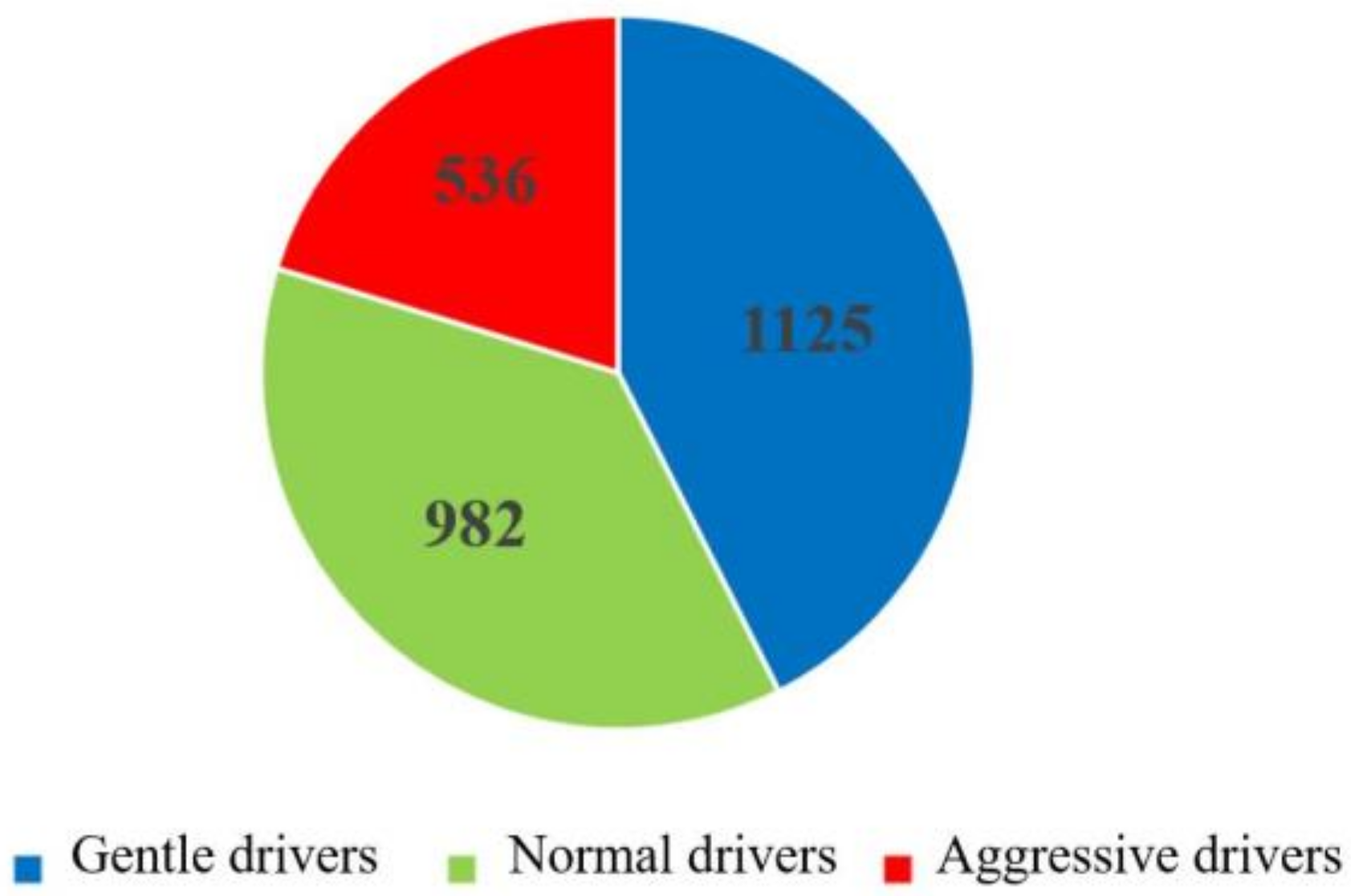
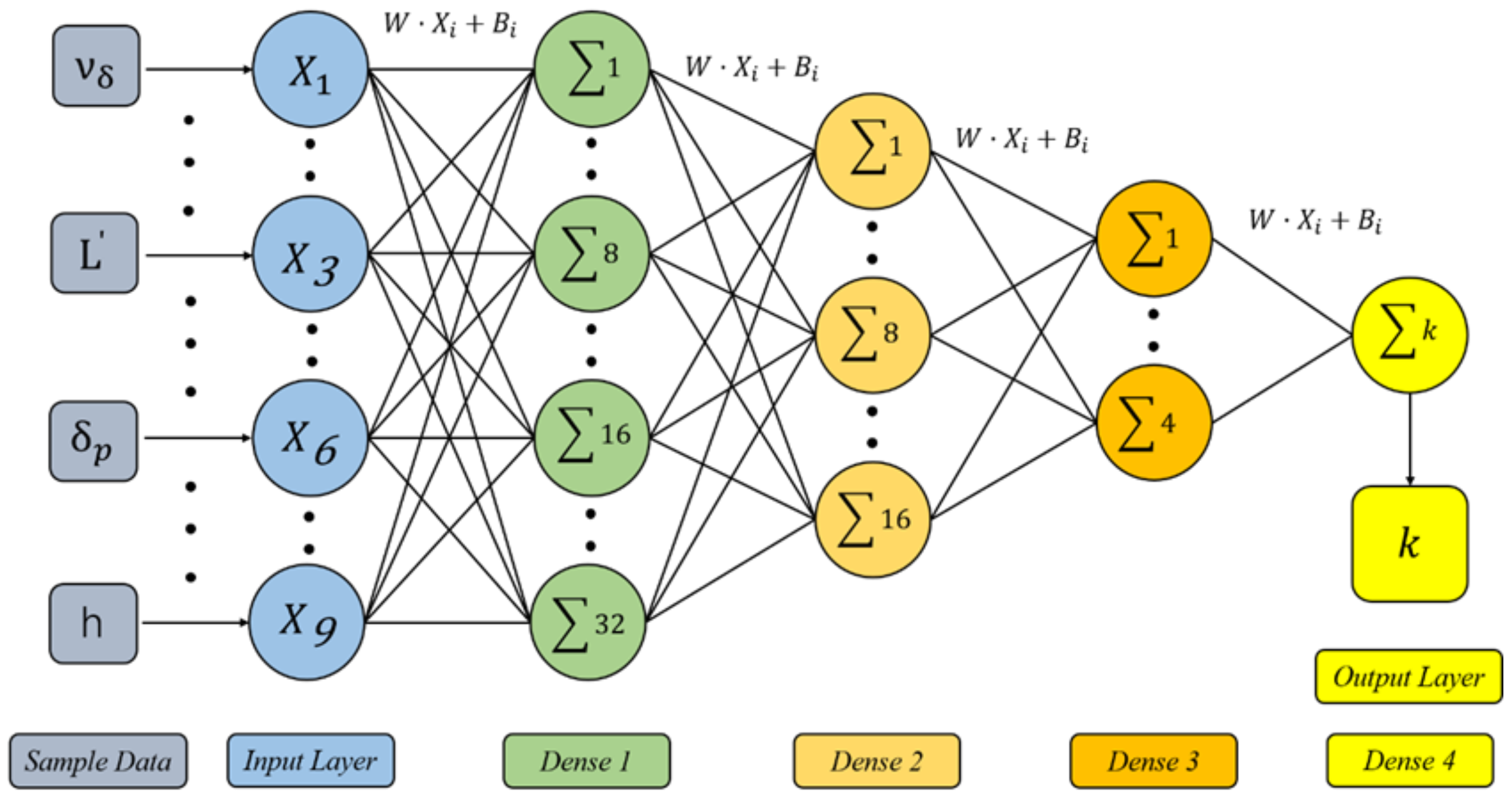
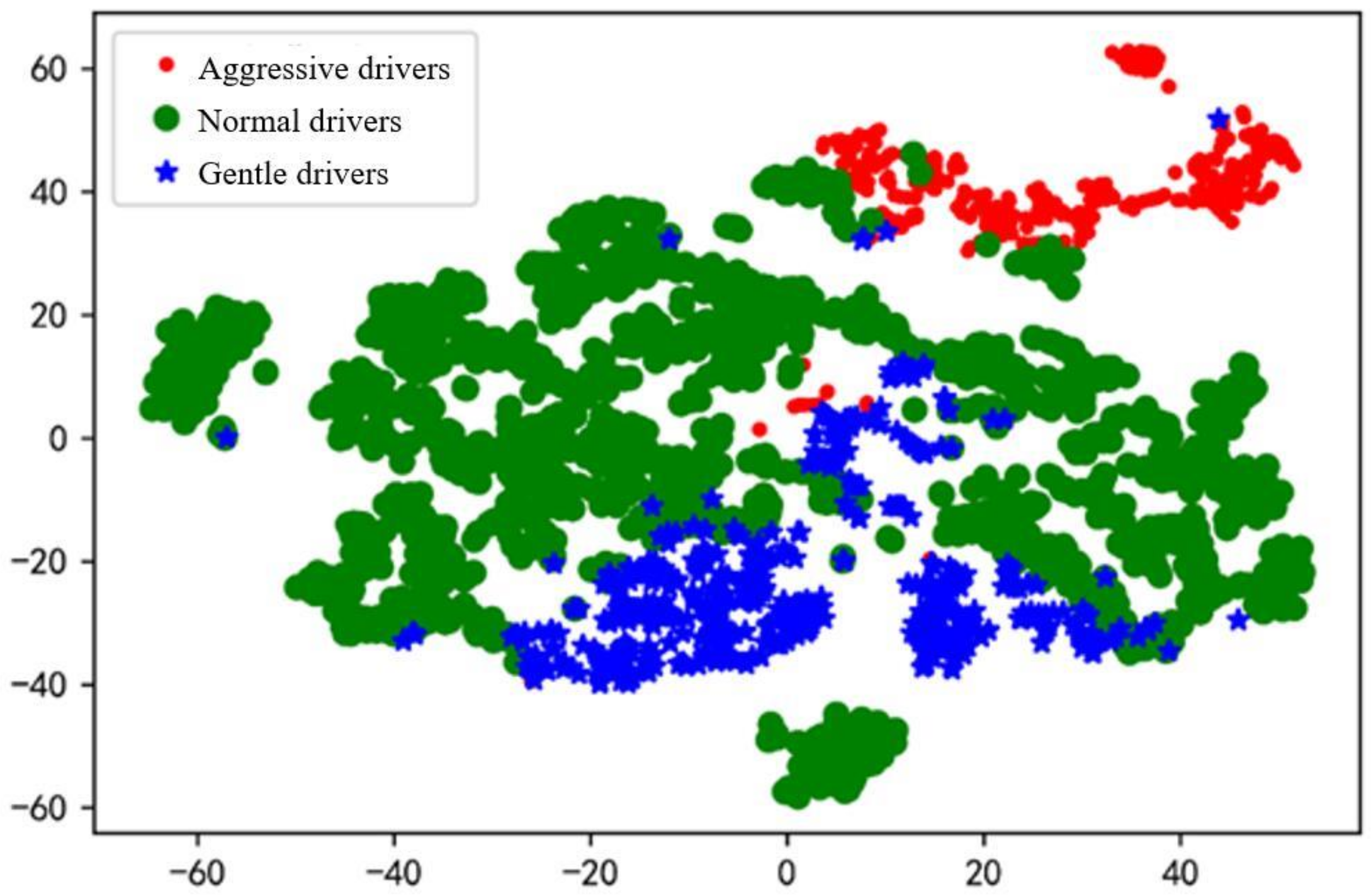
After the above-mentioned data screening and data processing, a total of 2642 sets of driver steering operation-related data were extracted from the driving test data of 30 drivers. These data were used for K-means cluster analysis and neural network model training.

3. Driver Characteristic Clustering and Identification

The driver characteristic identification algorithm was based on the K-means clustering analysis algorithm and the Keras neural network model. The main idea of the algorithm is as follows: the K-means clustering analysis algorithm classifies driver data, and the classified data will be imported into the Keras neural network model for learning, and then an identifier is built.

3.1. Driver Characteristic Clustering Based on K-Means

When applying the K-means algorithm to the driver characteristic classification problem, the value of k needs to be confirmed first. In this test, drivers were divided into three categories (gentle drivers, normal drivers and aggressive drivers); the value of k was set to 3. The data processing is described in Section 2. There were 2642 groups of effective steering operation data, and each group contained 9 data, including steering wheel angle, throttle opening and brake pressure.
The K-means algorithm uses distance to indicate the degree of similarity between data, among which Euclidean distance is the most commonly used. Therefore, Euclidean distance was selected as a measure of the similarity of driver characteristics, and the following formula could be obtained:
d i s t ( X i , C j ) = p = 1 m ( X i p C j p ) 2 X i = [ v δ σ δ L δ L P δ P v ¯ γ ¯ h ¯ ] T C j = [ v δ σ δ L δ L P δ P v ¯ γ ¯ h ¯ ] T
In Equation (10), X i represents an object in the data set; C j is a cluster center; m is the number of feature values in each group of data objects (m = 9); X i p and C j p are the corresponding eigenvalues.
The updated formula for cluster centers is as follows:
C j = 1 C j X i C j X i
Cj is the cluster center matrix; Xi is the data set matrix.
The K-means algorithm has two ways to stop the iteration. One is to stop the calculation when the number of iterations reaches the maximum of cycles; the other is to stop clustering when the function solution value is fixed. The convergence function is as follow:
J = min j = 1 3 X C j d i s t ( X , C j ) 2
In Equation (12), when J is the smallest, or continuously smaller than the set threshold, the iteration is terminated, and K-means clustering is completed.
After the derivation and calculation of the above formulas, the driver classification was completed. After clustering, the 2642 groups of experimental data were divided into 3 categories and could be used for neural network model training.

3.2. Identification of Drivers’ Characteristics Based on Keras

Among the methods of driver classification, the most commonly used method is the neural network. The Keras neural network can easily establish a model [42]. A neural network-based algorithm is a complex structure similar to the neurons of the human brain. The neural network is composed of a very large number of neurons, so the neural network can deal with the correlation between various parallel nonlinear data on a large scale. However, neural networks are limited by the quality and quantity of feature parameters in the entire dataset. For suitable datasets, neural network algorithms have strong model adaptation capabilities.
The structure of the Keras neural network model of this test is shown in Figure 5. The more layers of the neural network model, the stronger the nonlinear fitting ability and the richer the details of the target that can be extracted. The number of layers of the neural network model was reduced from 32 layers to 1 layer. The number of layers used in the modeling was mainly based on the test results of the data set and was determined according to the fit. The number of network layers was composed of 4 Dense. The units’ numbers of the first three layers were 32, 16 and 4, respectively. The last layer of the network had only one unit, which was used to output different driver categories. The softmax function commonly used in multiple classification problems was selected as the activation function. The input samples were data from the drivers’ steering maneuvers, and the output tags were the three categories of driver characteristics. W is the weight coefficient between layers, and Bi represents the bias term.
The loss function was set to the mean square error (MSE) and mean absolute error (MAE). The optimization solver was set to Rmsprop (Root Mean Square Prop), and the learning rate was set to 0.9. In the data set, the training set accounted for 70%, the validation set accounted for 20% and the test set accounted for 10%.

3.3. Analysis of Results

After K-means cluster analysis, the 2642 groups of data were divided into three different types of driver categories. In order to show the visualization effect after clustering, TSNE was used to reduce data dimensionality, and to select part of the data to draw the effect diagrams after clustering.
As shown in Figure 6 and Figure 7, after K-means clustering, drivers with larger driving characteristic parameters were defined as aggressive drivers; drivers with moderate driving characteristic parameters were defined as normal drivers; and drivers with small driving characteristic parameters were defined as gentle drivers. Therefore, the 2642 groups of driver data were divided into 1125 groups for gentle drivers, 982 groups for normal drivers and 536 groups for aggressive drivers. From the experimental results, gentle drivers and normal drivers accounted for 79.75% of the total, which showed that most drivers are more inclined to conservative driving operations during steering. A small number of drivers perform more intense driving operations, and they may have more proficient driving skills. From a macroperspective, the driver classification results of this test met the expectations of the test and can be used in neural network model training and verification.
As shown in Figure 8 and Figure 9, after 10 iterations of Keras model training, the training loss was less than 0.2, and the verification loss was about 0.3. The training accuracy was close to 95%, and the verification accuracy was close to 88%. During the training process, after 6 iterations, the verification loss gradually increased, and the model was over-fitted, which led to a decrease in the adaptive capacity of the model. In this test, the most suitable number of iterations was obtained by trying between different iterations. The prediction loss and prediction accuracy of the model could meet the requirements of use. Therefore, the process of identifying driver characteristics was completed.

4. Human-Like Path Planning Based on APF

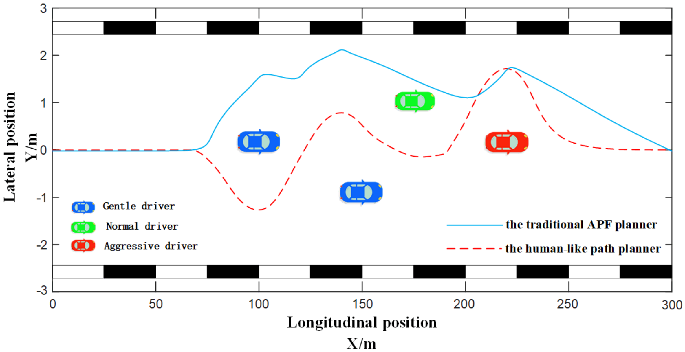
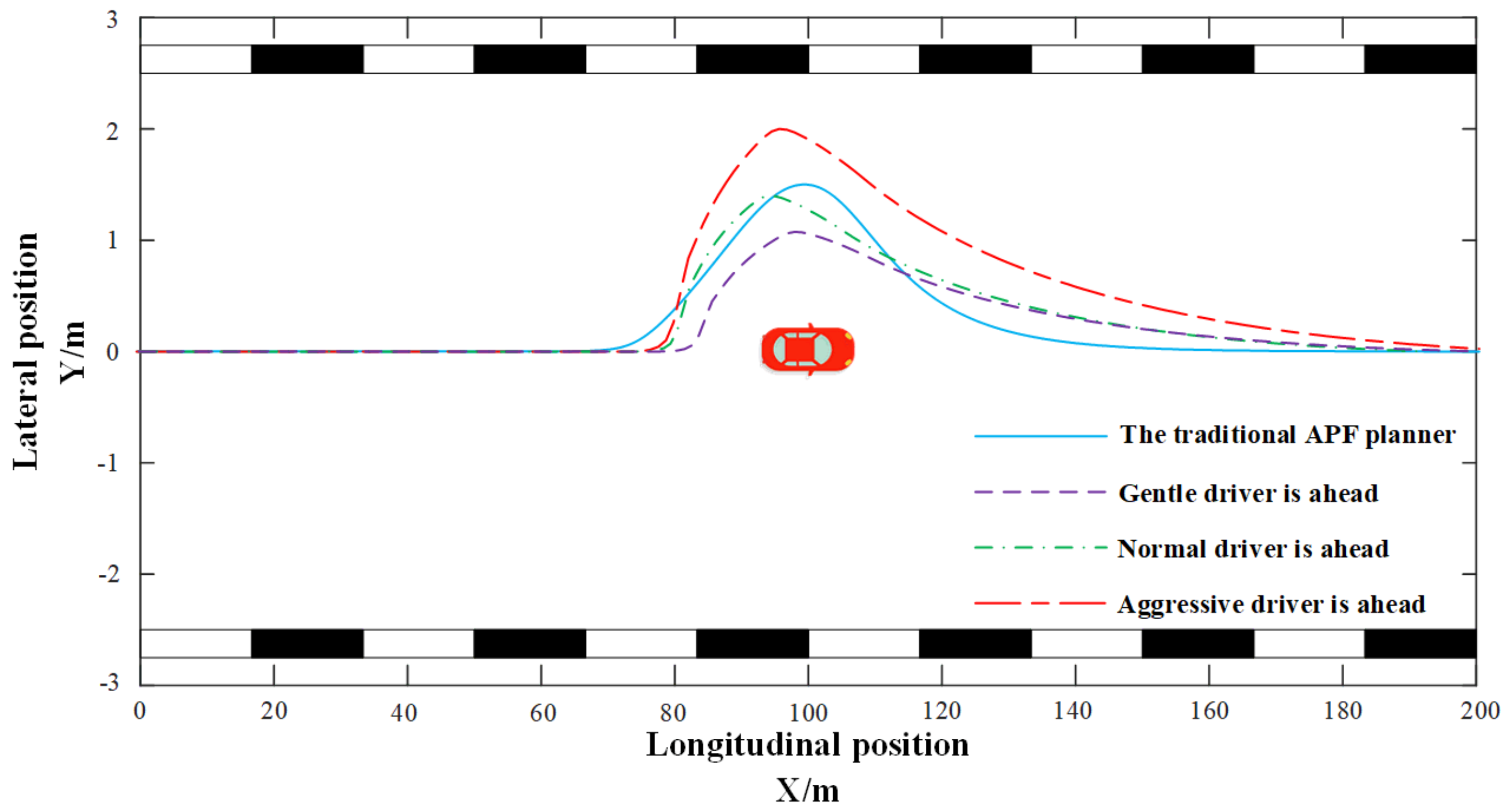
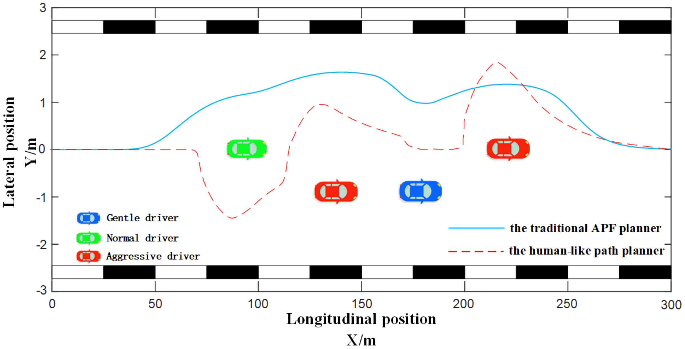
The design of the path planning controller based on driver characteristics and APF mainly considered the planning differences formed by the different repulsion potential fields generated by different drivers. In the path planning process of an autonomous vehicle, other manual driving vehicles exist as obstacles, the obstacle repulsion potential fields generated by different drivers are different. The road boundary also has a restraining effect, and the repulsive force field generated by the road boundary needs to be considered. The scenario designed in this section is the local path planning in the overtaking process. Combined with the drivers’ characteristics, three different driver obstacle repulsion potential fields and road boundary obstacle repulsion potential field were designed. Once autonomous vehicles could plan different paths based on different types of drivers in the traditional vehicles ahead, the path planning had the attribute of human-like decision making.

4.1. Artificial Potential Field Method (APF)

APF imitates the field concept of physics, fictionalizing a potential field in the scene. In the path planning, the end point was set as a gravitational potential field, and obstacles and road boundaries were set as repulsive potential fields; the controlled object moved under the influence of gravitational and repulsive forces in the potential fields, and finally reached the end [43].
The gravitational potential field was attractive to the controlled object. It had negative potential energy, and its function is expressed as follows:
U a t t ( X ) = 1 2 k a t t ρ m ( X , X g )
In Equation (13), U a t t ( X ) represents the gravitational field function; k a t t is the gravitational field factor; X is the position coordinate of the controlled object in the planning scene; X g is the position coordinate of the target point in the planning scene; ρ ( X , X g ) = X X g , which represents the Euclidean distance; m is the gravitational field factor.
Gravity was the negative gradient of the gravitational field function. It was the fastest descending direction of the gravitational field function. The formula of the gravitational function is as follows:
F a t t ( X ) = U a t t ( X ) = 1 2 k a t t ρ 2 ( X , X g ) = k a t t X X g
The repulsive force field had repulsive force on the controlled object. Its function is expressed as follows:
U r e p ( X ) = 1 2 k r e p ( 1 ρ ( X , X r ) 1 ρ r ) 2 ρ ( X , X r ) ρ r 0 ρ ( X , X r ) > ρ r
In Equation (15), U r e p ( X ) represents the repulsion function; k r e p is the gravitational field factor. X is the position coordinate of the controlled object in the planning scene; X r is the position coordinates of the obstacle in the planning scene; ρ r is the scope of the obstacle.
The repulsion is the negative gradient of the repulsion field function U r e p ( X ) . It represents the direction of the fastest decline in the repulsion potential field function, U r e p . The formula is:
F r e p ( X ) = U r e p ( X ) = k r e p ( 1 ρ ( X , X r ) 1 ρ r ) 1 ρ 2 ( X , X r ) ρ ( X , X r ) X ρ ( X , X r ) ρ r 0 ρ ( X , X r ) > ρ r
The gravitational potential field and the repulsive potential fields were combined to obtain the resultant potential field. The calculation rule followed the vector calculation:
U ( X ) = U a t t ( X ) + i = 1 n U r e p ( X )
In Equation (17), U ( X ) represents the resultant potential field of the artificial potential field; n represents the number of obstacles and road boundaries.
The formula of the resultant force is as follows:
F ( X ) = U ( X ) = F a t t ( X ) + F r e p ( X )
From Equations (17) and (18), the potential field potential energy and potential field force of the controlled object at each point in the planning scene could be calculated, and the controlled object moved in the direction with the fastest gradient drop under the influence of the situation force until it reached the target point.

4.2. Normalization of the Distances between the Vehicle and the Obstacles

The obstacle repulsion field is generally set to be circular. However, the situation is different in path planning. According to the actual driving conditions of a vehicle, it needs a larger repulsion potential field in the longitudinal and a smaller repulsion potential field in the lateral. Therefore, the repulsion field of a vehicle is similar to a diamond. If the radius of the repulsive force field is too large, the lateral distance of the vehicle during obstacle avoidance will be too large, which does not conform to actual driving habits and traffic laws; if the radius of the repulsive force field is too small, the longitudinal distance of the vehicle during obstacle avoidance will be insufficient, resulting in a risk of collision. The obstacle repulsion potential fields of a vehicle mainly depend on the speed and the maximum braking deceleration. The longitudinal safety distance is generally about tens of meters to one hundred meters, and the lateral safety distance is generally about a few meters. Therefore, the longitudinal and lateral distances of the vehicle obstacle repulsion potential field need to be normalized according to different safety distances. The formulas for the longitudinal safety distance and the lateral safety distance are as follows [44]:
X s = X min + u T + Δ u a 2 2 a max
Y s = Y min + ( u sin θ e + u 0 sin θ e ) T + Δ v a 2 2 a max
In Equations (19) and (20), X s is the vertical distance; X min is the minimum longitudinal distance; u is the longitudinal speed of the vehicle; T is a safe time interval, used to compensate vehicle response time; Δ u a is the longitudinal relative speed; a max is the maximum braking speed; Y s is the horizontal distance; Y min is the minimum lateral distance; u 0 is the longitudinal speed of the obstacle; θ e is the relative heading angle; Δ v a is the relative lateral velocity.
The following formulas were used to normalize the actual distances between the vehicle and obstacles:
X n = X a X s
Y n = Y a Y s
ρ n = X n 2 + Y n 2
In Equations (21)–(23), X n is the longitudinal normalized distance of the vehicle, X a is the actual longitudinal distance between the vehicle and the obstacle; Y n is the normalized distance of the vehicle laterally; Y a is the actual lateral distance between the vehicle and the obstacle; ρ n is the normalized distance between the vehicle and the obstacle.

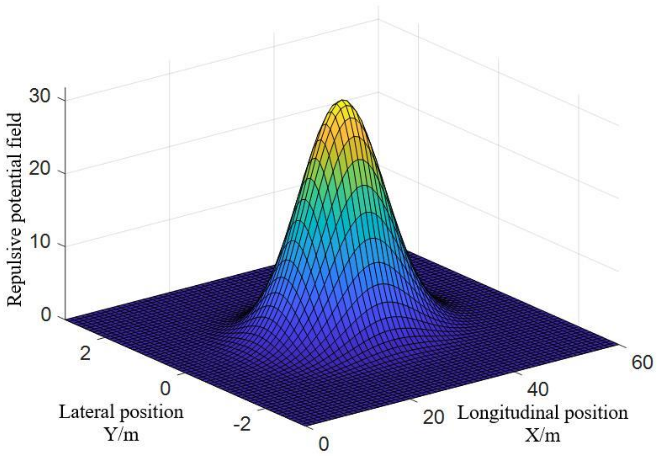
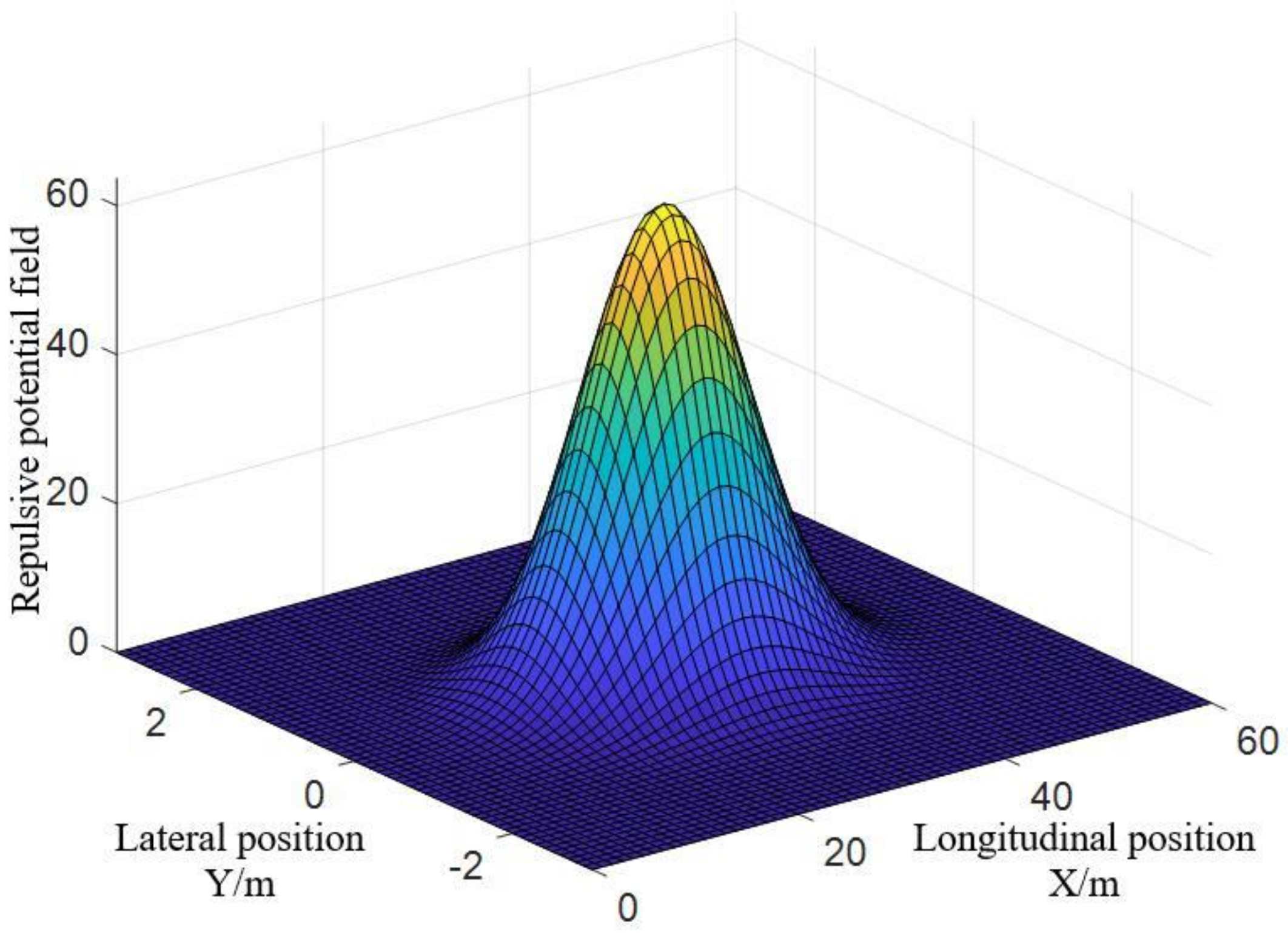
4.3. Repulsive Potential Field Function of Different Drivers

In the local path planning of overtaking scenes, different planning strategies should be adopted for different types of drivers. When a driver is of the aggressive type, his/her obstacle potential field should be set larger to reserve enough safe space; when a driver is of the gentle type, his/her obstacle potential field should be set smaller to facilitate quick overtaking. For different drivers, different repulsive gain coefficients need to be set, for which the formulas are as follows [43]:
U r e p g e n ( X ) = 1 2 k r e p g e n ( 1 ρ n ( X , X r ) 1 ρ r ) 2 ρ n ( X , X r ) ρ r 0 ρ n ( X , X r ) > ρ r
U r e p n o r ( X ) = 1 2 k r e p n o r ( 1 ρ n ( X , X r ) 1 ρ r ) 2 ρ n ( X , X r ) ρ r 0 ρ n ( X , X r ) > ρ r
U r e p a g g ( X ) = 1 2 k r e p a g g ( 1 ρ n ( X , X r ) 1 ρ r ) 2 ρ n ( X , X r ) ρ r 0 ρ n ( X , X r ) > ρ r
Equations (24)–(26) are formulas of the repulsive force potential fields of gentle drivers, normal drivers and aggressive drivers, respectively. After several attempts planning the path with different coefficients, the gain coefficients of the repulsive force potential field of gentle drivers, normal drivers and aggressive drivers were determined, respectively: k r e p g e n is the gain coefficient of gentle drivers’ repulsive force potential field, with a value of 5; k r e p n o r is the gain coefficient of normal drivers’ repulsive force potential field, with a value of 25; k r e p a g g is the gain coefficient of aggressive drivers’ repulsive force potential field, with a value of 50.

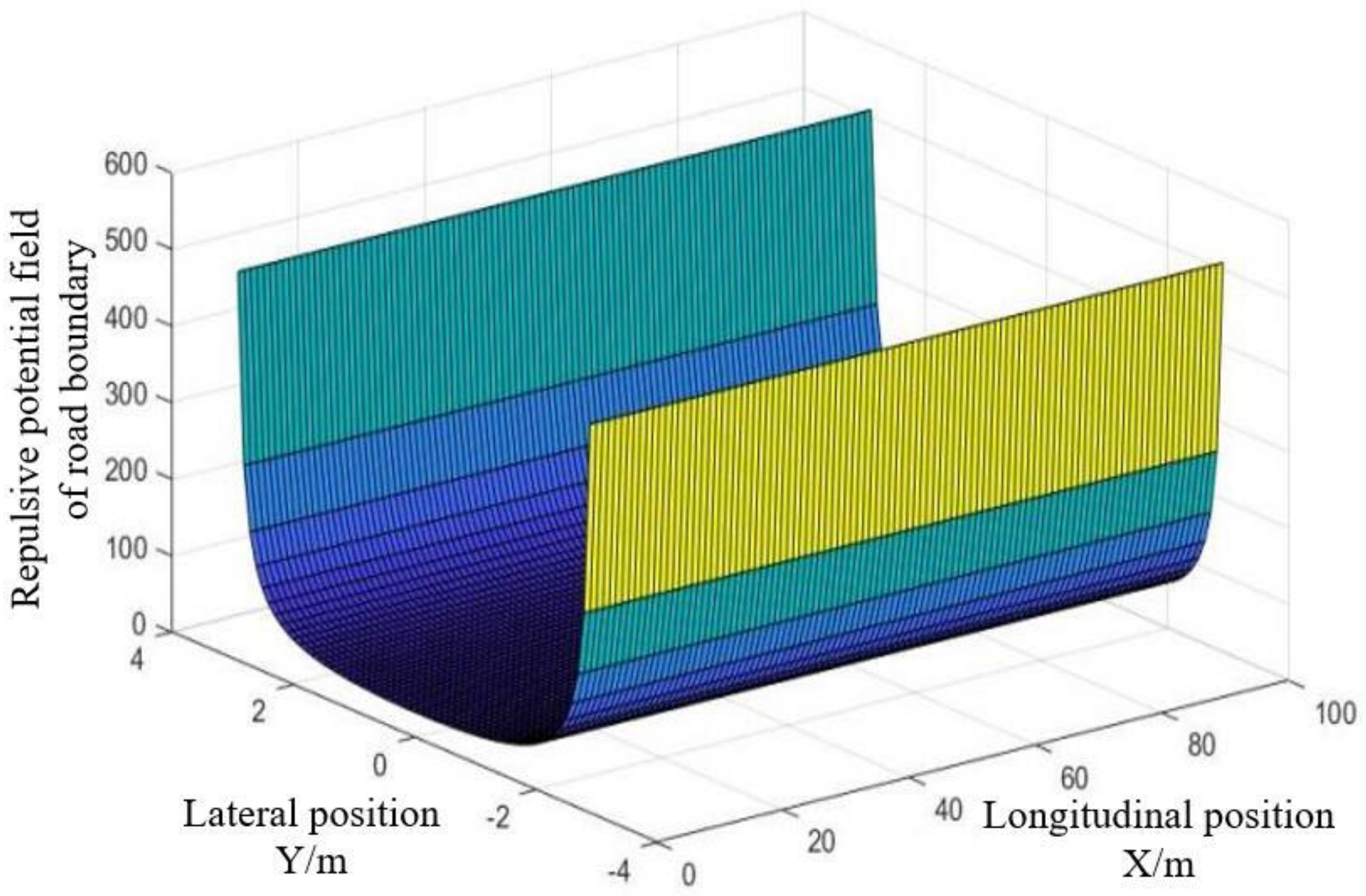
4.4. Road Boundary Repulsive Force Potential Field Function

Road constraints should also be taken into consideration. The planned path must not exceed the constraints of the road boundary, and the following function was selected as the repulsive potential field function of road boundary [43]:
U r e p r o a d ( Y l , Y r ) = k r e p l o a d ( 1 Y l 2 + 1 Y r 2 )
In Equation (27), U r e p r o a d ( Y l , Y r ) is the repulsive force field at the road boundary; k r e p l o a d is the gain coefficient of the road boundary repulsive force potential field, after several attempts planning the path with different coefficients, whose value was selected as 150; Y l is the distance between the vehicle and the left boundary of the road; Y r is the distance between the vehicle and the right boundary of the road.

5. Simulation and Result Analysis

According to the repulsive potential field function established in the previous section, the graphs of the repulsion potential field function were drawn, and on this basis, simulation tests of an individual driver and various drivers with different characteristics in overtaking scenes were carried out.

5.1. Driver Repulsive Potential Fields and Road Boundary Repulsive Potential Fields

Figure 10, Figure 11 and Figure 12 are the function graphs of the repulsive force potential fields of gentle drivers, normal drivers and aggressive drivers. k r e p g e n is the gain coefficient of gentle drivers’ repulsive force potential field, with a value of 5; k r e p n o r is the gain coefficient of normal drivers’ repulsive force potential field, with a value of 25; k r e p a g g is the gain coefficient of aggressive drivers’ repulsive force potential field, with a value of 50.
The graph of the road boundary repulsive potential field is shown in Figure 13, in which k r e p l o a d is the gain coefficient of the road boundary repulsive force potential field, with a value of 150. When the vehicle was close to the road boundary, the gradient of the repulsive force field increased sharply as the distance decreased; when the vehicle was far from the road boundary, as the distance increased, the repulsive force potential field gradient approached zero.

5.2. Individual Driver with Different Characteristics in Overtaking Scenes

The simulation was carried out in Matlab, the speed was set to 20 m/s and the road was set to be an expressway with a length of 200 m and a width of 6 m. Figure 14 shows the different planning paths made by the traditional APF planner and the human-like path planner when the types of the traditional vehicles’ drivers in front were gentle, normal or aggressive. The potential field function of the traditional APF was fixed, and the planning paths when facing different drivers were the same, which reflected that the traditional APF lacks adaptability. The human-like path planner reserved a small lateral distance in the overtaking scene with a gentle driver ahead; with a normal driver ahead, the planned path was similar to the traditional APFs; with an aggressive driver ahead, a larger lateral distance was reserved. IAPF can plan corresponding paths according to the different operating habits of the drivers in front, and had the functional attributes of human-like decision making. It can be seen from the figure that the planned route of the traditional APF could return to the driving route faster. This is because the repulsive potential field function of the traditional APF was similar to a circle, and there was no corresponding change in the longitudinal and lateral distance in path planning. The human-like decision-making path planner set different coefficients for the longitudinal distance and the lateral distance of the vehicle so that there were enough safe distances to return to the original driving route.

5.3. Various Driver with Different Characteristics in Overtaking Scenes

Figure 15 and Figure 16 show the overtaking path planning when various drivers coexisted in a traffic scene. The traditional APF could not plan a reasonable path due to the fixed potential field function. It approximated various drivers as an obstacle, and the planned paths were all as above, which did not conform to the actual situation. The human-like decision path planner provided different potential field functions according to different driver characteristics, to plan corresponding paths.
When there were different types of drivers in a traffic scene, the paths planned by the human-like decision-making path planner were smoother and more natural, which would avoid collisions with obstacles. In Figure 15, the overtaking path planned by the IPAF method reserved a lateral safety distance of about 1.5 m when overtaking a vehicle controlled by a gentle driver or a normal driver. During the recovery process, the longitudinal safety distance reserved when overtaking a vehicle operated by a normal driver was about 20 m more than the former. As the traditional APF method could not identify the types of drivers of the surrounding vehicles, the lateral and longitudinal safety distances reserved when overtaking green vehicles were too small, and the collision risk was high, and when overtaking two blue vehicles, too much safety distance was reserved, which caused the waste of traffic resources and easily caused congestion. In Figure 16, when using the IPAF method to plan the overtaking path, the lateral safety distances of 1, 1.5 and 2 m were reserved when overtaking vehicles controlled by gentle, normal and aggressive drivers, respectively. However, the traditional APF method reserved an excessively large safety distance (2 to 3 m) when overtaking the second and third vehicles in the figure, occupying too many road resources and easily causing congestion.
The simulation tests of an individual driver and various drivers with different characteristics in overtaking scenes showed that the curves of human-like path planning method were more reasonable than those of the traditional APFs; the proposed method can make a more effective path plan for autonomous vehicles according to the different driving styles of surrounding manual vehicles.

6. Conclusions

The deep learning method represented by the Keras neural network model was used in the path planning of autonomous vehicles, and the following conclusions were obtained:
(1)
The driver characteristic identification algorithm based on the K-means clustering analysis algorithm and Keras neural network model had a training accuracy close to 95% and a verification accuracy close to 88%, which could accurately classify the driving styles of different drivers.
(2)
The IAPF proposed by combining driver characteristic identification with traditional APF could plan more effective paths for autonomous vehicles according to the different driving styles of surrounding manual vehicles.
(3)
Based on the coupling of driver characteristics and APF, a human-like path planning controller was designed. The simulation tests of an individual driver and various drivers with different characteristics in overtaking scenes showed that the curves of the human-like path planning method were more reasonable and smoother than those of traditional APFs.
(4)
In the straight-line driving condition of the vehicle ahead, this paper combined the driver’s characteristic identification with APF to provide a better path to the overtaking path planning problem. In the future, we will also take the maneuver of surrounding vehicles into consideration to improve the adaptability of the IAPF.

Author Contributions

Conceptualization, F.L.; methodology, F.L. and L.Z.; software, S.W., T.W., L.Z. and Y.D.; validation, S.W. and Y.Z.; formal analysis, T.W.; investigation, F.L., Y.Z. and Y.D.; writing—Original Draft, S.W. and T.W.; writing—review & editing, F.L. and T.W.; supervision, F.L.; funding acquisition, F.L. All authors have read and agreed to the published version of the manuscript.

Funding

This research was funded by the Fundamental Research Funds for the Central Universities of China (grant number. NS2020016).

Data Availability Statement

The data presented in this study are available on reasonable request from the first author. The data are not publicly available due to privacy.

Conflicts of Interest

The authors declare that they have no known competing financial interests or personal relationships that could have appeared to influence the work reported in this paper.

References

  1. Thierry, D.; Victor, M.; Marie-Francine, M. Giving commands to a self-driving car: How to deal with uncertain situations? Eng. Appl. Artif. Intell. 2021, 103, 104257. [Google Scholar]
  2. Son, J.; Lee, H.; Choi, J. Driving Assistant Companion with Voice Interface Using Long Short-Term Memory Networks. IEEE Trans. Ind. Inform. 2019, 15, 582–590. [Google Scholar]
  3. Xu, Y.; Wang, X.; Li, W. GA-BPNN Based Hybrid Steering Control Approach for Unmanned Driving Electric Vehicle with In-Wheel Motors. IEEE/CAA J. Autom. Sin. 2020, 7, 178–186. [Google Scholar]
  4. Zhen, X.; Enze, Z.; Qingwei, C. Rotary unmanned aerial vehicles path planning in rough terrain based on multi-objective particle swarm optimization. J. Syst. Eng. Electron. 2020, 31, 130–141. [Google Scholar]
  5. Ren, G.; Zhang, Y.; Liu, H.; Zhang, K.; Hu, Y. A New Lane-Changing Model with Consideration of Driving Style. Int. J. Intell. Transp. Syst. Res. 2019, 17, 181–189. [Google Scholar] [CrossRef]
  6. Zhang, K.; Wang, J.; Chen, N.; Yin, G. A non-cooperative vehicle-to-vehicle trajectory-planning algorithm with consideration of driver’s characteristics. Proc. Inst. Mech. Eng. Part D J. Automob. Eng. 2018, 233, 095440701878339. [Google Scholar] [CrossRef]
  7. Jarnea, A.D.; Dobrescu, R.; Popescu, D.; Ichim, L. Advanced driver assistance system for overtaking maneuver on a highway. In Proceedings of the International Conference on System Theory, IEEE, Cheile Gradistei, Romania, 14–16 October 2015. [Google Scholar]
  8. Taheri, S.M.; Matsushita, K.; Sasaki, M. Virtual Reality Driving Simulation for Measuring Driver Behavior and Characteristics. J. Transp. Technol. 2017, 7, 123–132. [Google Scholar] [CrossRef] [Green Version]
  9. Rongben, W.; Lie, G.; Bingliang, T.; Lisheng, J. Monitoring Mouth Movement for Driver Fatigue or Distraction with One Camera. In Proceedings of the 7th International IEEE Conference on Intelligent Transportation Systems, Washington, WA, USA, 3–6 October 2004; pp. 314–319. [Google Scholar]
  10. El Falou, W.; Duchêne, J.; Grabisch, M.; Hewson, D.; Langeron, Y.; Lino, F. Evaluation of Driver Discomfort During Long-Duration Car Driving. Appl. Ergon. 2003, 34, 249–255. [Google Scholar] [CrossRef]
  11. Lei, Y.; Liu, K.; Fu, Y.; Li, X.; Liu, Z.; Sun, S. Research on Driving Style Recognition Method Based on Driver’s Dynamic Demand. Adv. Mech. Eng. 2016, 8, 1–14. [Google Scholar] [CrossRef] [Green Version]
  12. Daimon, T.; Nishimura, M.; Kawashima, H. Study of Drivers’ Behavioral Characteristics for Designing Interfaces of In-Vehicle Navigation Systems Based on National and Regional Factors. JSAE Rev. 2010, 21, 379–384. [Google Scholar] [CrossRef]
  13. Yoon, S.; Yoon, S.E.; Lee, U.; Shim, D.H. Recursive path planning using reduced states for car-like vehicles on grid maps. IEEE Trans. Intell. Transp. Syst. 2015, 16, 2797–2813. [Google Scholar] [CrossRef]
  14. Yijing, W.; Zhengxuan, L.; Zhiqiang, Z.; Zheng, L. Local path planning of autonomous vehicles based on A* algorithm with equal-step sampling. In Proceedings of the 37th Chinese Control Conference, Wuhan, China, 25–27 July 2018; pp. 7828–7833. [Google Scholar]
  15. Du, M.; Chen, J.; Zhao, P.; Liang, H.; Xin, Y.; Mei, T. An improved RRT-based motion planner for autonomous vehicle in cluttered environments. In Proceedings of the IEEE International Conference on Robotics and Automation, Hong Kong, China, 31 May–7 June 2016; pp. 4674–4679. [Google Scholar]
  16. Moses, E.D.B.; Anitha, G. Goal directed approach to autonomous motion planning for unmanned vehicles. Def. Sci. J. 2017, 67, 45–49. [Google Scholar] [CrossRef] [Green Version]
  17. Daily, R.; Bevly, D.M. Harmonic potential field path planning for high speed vehicles. In Proceedings of the American Control Conference, Seattle, WA, USA, 11–13 June 2018; pp. 4609–4614. [Google Scholar]
  18. Woo, H.; Ji, Y.; Kono, H.; Tamura, Y.; Kuroda, Y.; Sugano, T.; Yamamoto, Y.; Yamashita, A.; Asama, H. Automatic detection method of lane-changing intentions based on relationship with adjacent vehicles using artificial potential fields. Int. J. Automot. Eng. 2016, 7, 127–134. [Google Scholar] [CrossRef] [Green Version]
  19. Hou, P.; Pan, H.; Guo, C. Simulation research for mobile robot path planning based on improved artificial potential field method recommended by the AsiaSim. Int. J. Modeling Simul. Sci. Comput. 2017, 8, 1750046. [Google Scholar] [CrossRef]
  20. Steiner, J.A.; He, X.; Bourne, J.R.; Leang, K.K. Open-sector rapid-reactive collision avoidance: Application in aerial robot navigation through outdoor unstructured environments. Robot. Auton. Syst. 2019, 112, 211–220. [Google Scholar] [CrossRef]
  21. Borenstein, J.; Koren, Y. The vector field histogram-fast obstacle avoidance for mobile robots. IEEE Trans. Robot. Autom. 1991, 7, 278–288. [Google Scholar] [CrossRef] [Green Version]
  22. Mujahed, M.; Fischer, D.; Mertsching, B. Admissible gap navigation: A new collision avoidance approach. Robot. Auton. Syst. 2018, 103, 93–110. [Google Scholar] [CrossRef]
  23. Rubio-Sierra, C.; Domínguez, D.; Gonzalo, J.; Escapa, A. Path planner for autonomous exploration of underground mines by aerial vehicles. Sensors 2020, 20, 4259. [Google Scholar] [CrossRef] [PubMed]
  24. Hart, P.E.; Nilsson, N.J.; Raphael, B. A formal basis for the heuristic determination of minimum cost paths. IEEE Trans. Syst. Sci. Cybern. 1968, 4, 100–107. [Google Scholar] [CrossRef]
  25. Elbanhawi, M.; Simic, M. Sampling-based robot motion planning: A review. IEEE Access 2014, 2, 56–77. [Google Scholar] [CrossRef]
  26. Pérez-Hurtado, I.; Martínez-del-Amor, M.Á.; Zhang, G.; Neri, F.; Pérez-Jiménez, M.J. A membrane parallel rapidly-exploring random tree algorithm for robotic motion planning. Integr. Comput. -Aided Eng. 2020, 27, 121–138. [Google Scholar] [CrossRef]
  27. Gan, Y.; Zhang, B.; Ke, C.; Zhu, X.; He, W.; Ihara, T. Research on Robot Motion Planning Based on RRT Algorithm with Nonholonomic Constraints. Neural Processing Lett. 2021, 53, 3011–3029. [Google Scholar] [CrossRef]
  28. Masahiro, I.; Toshinobu, T.; Etsujiro, I. Analysis of cooking recipes written in Japanese and motion planning for cooking robot. ROBOMECH J. 2021, 8, 17. [Google Scholar]
  29. Khatib, O. Real-time obstacle avoidance for manipulators and mobile robots. In Proceedings of the IEEE International Conference on Robotics and Automation, St. Louis, MO, USA, 25–28 March 1985; pp. 500–505. [Google Scholar]
  30. Liu, C.; Lee, S.; Varnhagen, S.; Tseng, H.E. Path planning for autonomous vehicles using model predictive control. In Proceedings of the IEEE Intelligent Vehicles Symposium, Los Angeles, CA, USA, 11–14 June 2017; pp. 174–179. [Google Scholar]
  31. Abbas, M.A.; Milman, R.; Eklund, J.M. Obstacle avoidance in real time with nonlinear model predictive control of autonomous vehicles. Can. J. Electr. Comput. Eng. 2017, 40, 12–22. [Google Scholar] [CrossRef]
  32. Guo, H.; Shen, C.; Zhang, H.; Chen, H.; Jia, R. Simultaneous trajectory planning and tracking using an MPC method for cyber-physical systems: A case study of obstacle avoidance for an intelligent vehicle. IEEE Trans. Ind. Inform. 2018, 14, 4273–4283. [Google Scholar] [CrossRef]
  33. Altché, F.; Polack, P.; de La Fortelle, A. High-speed trajectory planning for autonomous vehicles using a simple dynamic model. In Proceedings of the IEEE 20th International Conference on Intelligent Transportation Systems, Yokohama, Japan, 16–19 October 2017; pp. 1–7. [Google Scholar]
  34. Gutjahr, B.; Gröll, L.; Werling, M. Lateral vehicle trajectory optimization using constrained linear time-varying MPC. IEEE Trans. Intell. Transp. Syst. 2017, 18, 1586–1595. [Google Scholar] [CrossRef]
  35. Huang, Z.; Wu, Q.; Ma, J.; Fan, S. An APF and MPC combined collaborative driving controller using vehicular communication technologies. Chaos Solitons Fractals 2016, 89, 232–242. [Google Scholar] [CrossRef]
  36. Ji, J.; Khajepour, A.; Melek, W.W.; Huang, Y. Path planning and tracking for vehicle collision avoidance based on model predictive control with multiconstraints. IEEE Trans. Veh. Technol. 2017, 66, 952–964. [Google Scholar] [CrossRef]
  37. Huang, Z.; Chu, D.; Wu, C.; He, Y. Path planning and cooperative control for automated vehicle platoon using hybrid automata. IEEE Trans. Intell. Transp. Syst. 2019, 20, 959–974. [Google Scholar] [CrossRef]
  38. Li, H.Z.; Li, L.; Song, J.; Yu, L.Y. Comprehensive Lateral Driver Model for Critical Maneuvering Conditions. Int. J. Automot. Technol. 2011, 12, 679–686. [Google Scholar] [CrossRef]
  39. Geng, G.; Wu, Z.; Jiang, H.; Sun, L.; Duan, C. Study on Path Planning Method for Imitating the Lane-Changing Operation of Excellent Drivers. Appl. Sci. 2018, 8, 814. [Google Scholar] [CrossRef] [Green Version]
  40. Zhang, L.; Wang, J.; Yang, F.; Li, K. A Quantification Method of Driver Characteristics Based on Driver Behavior Questionnaire. In Proceedings of the IEEE Intelligent Vehicles Symposium, Xi’an, China, 3–5 June 2009; pp. 616–620. [Google Scholar]
  41. Liu, F. Humanoid Decision-Making and Path-Planning for Lane-Changing of Unmanned Ground Vehicle on Highway; Jilin University: Changchun, China, 2019. [Google Scholar]
  42. Douglass, M. Hands-On Machine Learning with Scikit-Learn, Keras, and Tensorflow, 2nd Edition. Phys. Eng. Sci. Med. 2020, 43, 1135–1136. [Google Scholar] [CrossRef]
  43. Chen, Y. Vehicle Obstacle Avoidance Path Planning and Tracking Control Based on Adaptive Model Predictive Control, Nanjing University of Aeronautics and Astronautics: Nanjing, China, 2020.
  44. Kesting, A.; Treiber, M.; Schönhof, M.; Helbing, D. Adaptive Cruise Control Design for Active Congestion Avoidance. Transp. Res. Part C Emerg. Technol. 2008, 16, 668–683. [Google Scholar] [CrossRef]
Figure 1. Prescan and Matlab joint simulation platform.
Actuators 11 00052 g001
Figure 2. Driving scene in Perscan.
Actuators 11 00052 g002
Figure 3. The driver’s viewing point.
Actuators 11 00052 g003
Figure 4. The drivers’ personalized data collection test.
Actuators 11 00052 g004
Figure 5. Construction of Keras neural network model.
Actuators 11 00052 g005
Figure 6. Driver category after K-means clustering.
Actuators 11 00052 g006
Figure 7. Distribution of different driver types.
Actuators 11 00052 g007
Figure 8. Training loss and verification loss.
Actuators 11 00052 g008
Figure 9. Training accuracy and verification accuracy.
Actuators 11 00052 g009
Figure 10. Repulsive potential field of gentle drivers.
Actuators 11 00052 g010
Figure 11. Repulsive potential field of normal drivers.
Actuators 11 00052 g011
Figure 12. Repulsive potential field of aggressive drivers.
Actuators 11 00052 g012
Figure 13. Repulsive potential field of road boundary.
Actuators 11 00052 g013
Figure 14. Path planning in overtaking scenes with different drivers.
Actuators 11 00052 g014
Figure 15. Path planning in overtaking scenes A with various drivers.
Actuators 11 00052 g015
Figure 16. Path planning in overtaking scenes B with various drivers.
Actuators 11 00052 g016
Table 1. Test sample A.
Age18–2525–3535–50
Gender
Male398
Female244
Total51312
Table 2. Test Sample B.
Age18–2525–3535–50
Driving
Experience
0–3 years133
3–6 years255
>6 years254
Total51312
Publisher’s Note: MDPI stays neutral with regard to jurisdictional claims in published maps and institutional affiliations.

