PSO-Based Variable Parameter Linear Quadratic Regulator for Articulated Vehicles Snaking Oscillation Yaw Motion Control

Abstract

In this paper, the seven degrees of freedom (DOF) nonlinear system model of articulated vehicles, including the vehicle dynamics model, tire and hydraulic steering system model, and the linearized ideal reference model, is constructed. A layered stability controller for the articulated vehicle is built. The particle swarm optimization (PSO)-based variable parameter linear quadratic regulator (LQR) for the upper-level yaw torque controller and the lower-level torque distributor based on the principle of the minimum tire utilization are established. The effectiveness of the LQR upper-level yaw torque controller for an articulated vehicle at different speeds and control references are compared and analyzed through feedforward and feedback control. We optimize the parameters in the LQR controller using PSO and verify the improvement in the controller’s performance with optimized parameters. Overall, the effect of front and rear-integrated control is best, followed by rear-based and front-based control. The PSO algorithm to optimize the LQR controller parameters for snaking oscillation control is effective.

1. Introduction

Due to their small radius, excellent maneuverability, and wide adaptability, articulated vehicles are widely used in agriculture, forestry, construction, rescue and military, and other fields [1,2]. Since articulated vehicles are special configurations where a hydraulic steering system connects two separate bodies, the lateral stability is poor, especially at high speeds. The articulated vehicles show the instability phenomenon in forms such as snaking oscillation. Corresponding studies on snaking oscillation and influencing factors have been conducted by relevant scholars [3,4,5]. These studies reinforce that snaking oscillation can limit the speed of articulated vehicles, increase the operational burden and hazards for drivers, and reduce the operational efficiency of articulated vehicles. Therefore, it is necessary and meaningful to study the snaking oscillation suppression of articulated vehicles.

The study of snaking oscillation suppression of articulated vehicles can be categorized into two main research methods. The passive method includes improving the hydraulic steering system [6,7], optimizing the friction and damping of articulated points, and locking the differential [8]. The other is the active control method, which includes hydraulic system control [9], differential braking control, direct transverse moment control [10], and other active control methods. Due to the perfection of the electric drive, the distributed drive is realized, and the controllability of the vehicle chassis is greatly improved. The corresponding control strategies and algorithms improve vehicle stability under complex working conditions and avoid the adverse effects of passive control, such as limited control effects and large energy consumption. The most current applications for distributed electric drive vehicle stability active control are direct yaw control and the layered control mode [11,12]. The upper generalized force-calculation layer, based on the driver’s intention and the vehicle’s current state, calculates the longitudinal forces and yaw moments that should be applied to the vehicle through optimization algorithms. In the lower moment distribution layer, the generalized forces calculated in the upper layer are coordinately distributed to the wheels’ driving forces by various algorithms [13,14,15,16,17].

Azad designed a robust state feedback controller to suppress snaking oscillation by calculating and adjusting the parameters of the robust controller [1,18]. Wang compared the control effect of a single PID controller with a dual PID controller by establishing a linear dynamics model reflecting the lateral characteristics of the vehicle. The simulation results showed that the dual PID controller could provide a faster response and better stability effects [19]. Mehdi Abroshan designed an MPC controller for differential braking of tractor and trailer to suppress Jackknifing and snaking instability modes [20]. Piotr Dudziński constructed an articulated vehicle’s stability function to achieve snaking oscillation suppression as well as straight-line retention by controlling the front wheel braking torque magnitude and braking time [21]. Cheng applied the sliding mode control algorithm in the upper layer to calculate the demanded yaw moment and applied the BP artificial neural network to design the lower moment distribution layer [22]. Gao established a layered LQR stability controller in the form of feedforward and feedback using the yaw velocity and side slip angle as control parameters. The front-based control effect and the rear-based control effect were investigated. Overall, the front-based control effect was better [23]. Xu used the MPC algorithm to control the vehicle yaw velocity and side slip angle and compared the effect with the LQR algorithm [24]. In the existing studies, the control of articulated vehicles is based on the front or rear body. There is no comprehensive study on front and integrated rear control. In studying some control algorithms for articulated vehicles, the selection of parameters relies on empirical selection. This may not be conducive to establishing the best control of the controller and waste a significant amount of time adjusting parameters.

This paper uses optimal control theory and the layered control method to establish the controller for articulated vehicle snaking suppression. The nonlinear dynamics model for articulated vehicles and the linearized reference model are developed. The LQR upper yaw torque calculating layer and the lower level torque distributor based on the principle of minimum tire utilization are established. The effect of the articulated vehicle snaking oscillation controller is improved by optimizing each parameter in the LQR controller through PSO. The effects of snaking oscillation suppression of articulated vehicles are compared and analyzed under two working conditions of low and high speeds based on three control bases: front-based control, rear-based control, and front and rear integrated control.

2. Modeling of Nonlinear Systems for Articulated Vehicles

2.1. Vehicle Dynamics Analysis and Modeling

The articulated vehicle dynamics model is the basis of dynamics control. Therefore, a 7 DOF articulated vehicle nonlinear system model containing the vehicle dynamics model, the tire model, and the hydraulic steering model is established. The articulated vehicle dynamics model is simplified as follows based on this study’s research objectives:

(1)

The front and rear body centers are located on the longitudinal central axis, and the vehicle is symmetrical with respect to the longitudinal central axis;

(2)

The influence of the tire camber angle and return torque are disregarded;

(3)

Air resistance is disregarded, and the road surface is flat and two-dimensional.

The articulated vehicle dynamics model is shown in Figure 1; the related quantities applied in this paper are in the nomenclature. The force analysis of the articulated vehicle is carried out to obtain the equilibrium equations for the lateral, longitudinal, and yaw of the front and rear vehicles. After simplification, the articulated vehicle dynamics equations are shown in Equation (1). The tire force and the equivalent moment of the hydraulic steering system acting on the articulation point in the equation can be obtained from the tire model and the hydraulic steering system model. The initial Newtonian mechanics’ equations and the simplification process are shown in Appendix A.

$$\{\begin{array}{l}\left(m_1+m_2\right){\dot{v}}_{x1}=\left(m_2+m_1\right)w_1{v}_{y_1}+m_2{L}_4{\dot{w}}_2\mathit{sin}\beta -m_2{L}_2{w}_1{}^2-m_2{L}_4{w}_2^2\mathit{cos}\beta +\\ F_{x1}+F_{x2}+\left(F_{x3}+F_{x4}\right)\mathit{cos}\beta +\left(F_{y3}+F_{y4}\right)\mathit{sin}\beta \\ \left(m_1+m_2\right){\dot{v}}_{y1}=m_2{L}_2{\dot{w}}_1-\left(m_1+m_2\right)w_1{v}_{x1}+m_2{L}_4{\dot{w}}_2\mathit{cos}\beta +m_2{L}_4{w}_2{}^2\mathit{sin}\beta +\\ F_{y1}+F_{y2}+\left(F_{y3}+F_{y4}\right)\mathit{cos}\beta -\left(F_{x3}+F_{x4}\right)\mathit{sin}\beta \\ I_1{\dot{w}}_1=M_{O1}+\left(F_{x1}-F_{x2}\right)B+\left(F_{y1}+F_{y2}\right)\left(L_1+L_2\right)-m_1\left({\dot{v}}_{y1}+v_{x1}{\omega }_1\right)L_2\\ I_2{\dot{\omega }}_2=-M_{O2}+\left(F_{x3}-F_{x4}\right)B-\left(F_{y3}+F_{y4}\right)L_3+\left(F_{y1}+F_{y2}\right)L_4\mathit{cos}\beta \\ +\left(F_{x1}+F_{x2}\right)L_4\mathit{sin}\beta -m_1\left({\dot{v}}_{y1}+v_{x1}{\omega }_1\right)L_4\mathit{cos}\beta -m_1\left({\dot{v}}_{x1}-v_{y1}{\omega }_1\right)L_4\mathit{sin}\beta \end{array}$$

(1)

The vertical force of each tire will change with the change of the articulated angle, and the lateral and longitudinal acceleration will cause axial load transfer. Therefore, in addition to its gravity, the transferred load should be distributed. The analysis of the articulated vehicle’s vertical force is shown in Figure 2. The vertical force of each tire is shown in Equation (2), and the specific calculation process is included in Appendix A.

$$\{\begin{array}{c}{F}_{z1}=\frac{L_{lr}}{L_{lf}+L_{lr}}\frac{B\mathit{cos}{\theta }_2+△B}{2B\mathit{cos}{\theta }_2}\left(m_1+m_2\right)g-\frac{\left(B\mathit{cos}{\theta }_2+△B\right)\left(m_1+m_2\right)a_x^{\text{'}}\mathit{h}}{2BL\text{'}\mathit{cos}{\theta }_2}+\frac{L_{lr}}{L_{lf}+L_{lr}}\frac{\left(m_1+m_2\right)a_y^{\text{'}}\mathit{h}}{2B\mathit{cos}{\theta }_2}\\ F_{z2}=\frac{L_{rr}}{L_{rf}+L_{rr}}\frac{B\mathit{cos}{\theta }_2-△B}{2B\mathit{cos}{\theta }_2}\left(m_1+m_2\right)g-\frac{\left(B\mathit{cos}{\theta }_2-△B\right)\left(m_1+m_2\right)a_x^{\text{'}}\mathit{h}}{2BL\text{'}\mathit{cos}{\theta }_2}-\frac{L_{rr}}{L_{rf}+L_{rr}}\frac{\left(m_1+m_2\right)a_y^{\text{'}}\mathit{h}}{2B\mathit{cos}{\theta }_2}\\ F_{z3}=\frac{L_{lf}}{L_{lf}+L_{lr}}\frac{B\mathit{cos}{\theta }_2+△B}{2B\mathit{cos}{\theta }_2}\left(m_1+m_2\right)g+\frac{\left(B\mathit{cos}{\theta }_2+△B\right)\left(m_1+m_2\right)a_x^{\text{'}}\mathit{h}}{2BL\text{'}\mathit{cos}{\theta }_2}+\frac{L_{lf}}{L_{lf}+L_{lr}}\frac{\left(m_1+m_2\right)a_y^{\text{'}}\mathit{h}}{2B\mathit{cos}{\theta }_2}\\ F_{z4}=\frac{L_{rf}}{L_{rf}+L_{rr}}\frac{B\mathit{cos}{\theta }_2-△B}{2B\mathit{cos}{\theta }_2}\left(m_1+m_2\right)g+\frac{\left(B\mathit{cos}{\theta }_2-△B\right)\left(m_1+m_2\right)a_x^{\text{'}}\mathit{h}}{2BL\text{'}\mathit{cos}{\theta }_2}-\frac{L_{rf}}{L_{rf}+L_{rr}}\frac{\left(m_1+m_2\right)a_y^{\text{'}}\mathit{h}}{2B\mathit{cos}{\theta }_2}\end{array}$$

(2)

2.2. Tire Models

This study uses the Dugoff tire model, which complements the elastic base analysis model established by Fiala and the integrated lateral force–vertical force model of Pacejka and Sharp. The tire model provides a method to calculate the forces under the combined action of lateral and longitudinal forces. The characteristics are fast computation and require fewer parameters. The lateral and longitudinal forces of the tire can be obtained from the vertical force of the tire, the tire side slip angle, and the longitudinal slip rate. The model equations are as follows:

$$\{\begin{array}{c}{F}_x=C_{\sigma }\frac{S_{ti}}{1+S_{ti}}f\left(\lambda \right)\\ F_y=C_{\alpha }\frac{\tan (\alpha )}{1+S_{ti}}f\left(\lambda \right)\end{array}$$

(3)

where $\lambda =\frac{\mu F_z\left(1+S_{ti}\right)}{2{\{{\left(C_{\sigma }{S}_{ti}\right)}^2+{\left(C_{\sigma }\tan (\alpha )\right)}^2\}}^{1/2}} f\left(\lambda \right)=\{\begin{array}{l}\left(2-\lambda \right)\lambda \lambda <1\\ 1 \lambda ⩾1\end{array}$. Other parameters and the calculation process are included in Appendix A.

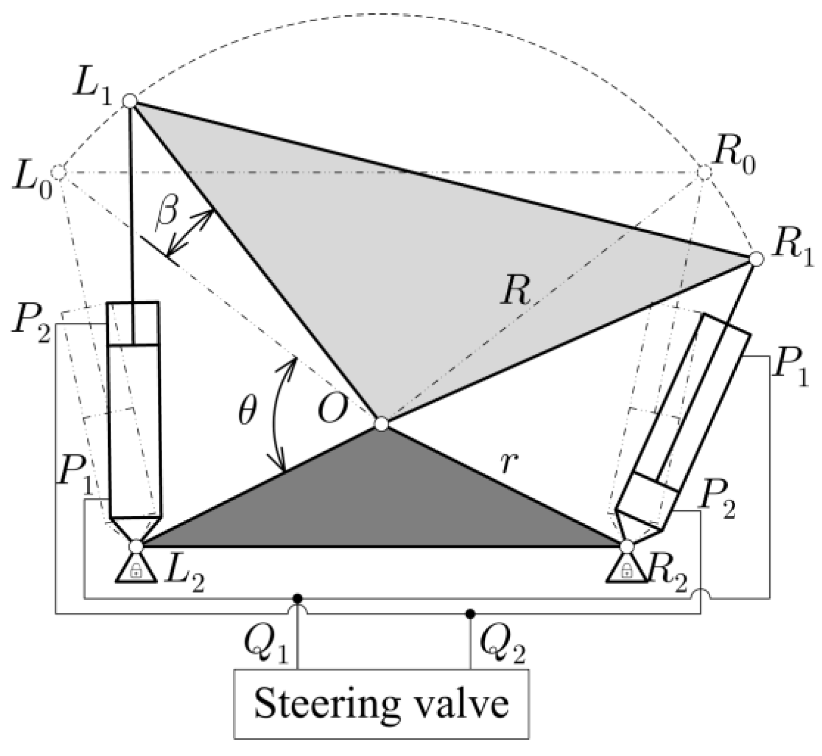
2.3. Hydraulic Steering System Model

The hydraulic steering system model is shown in Figure 3. When articulated vehicles travel in a straight line or at a fixed radius, the inlet and outlet ports of the steering valve are closed, and the hydraulic steering system is equivalent to a torsion spring acting at the steering hinge point and connecting the front and rear bodies.

The left and right hydraulic cylinder forces are as follows:

$$\{\begin{array}{c}{F}_L=P_1{A}_1-P_2{A}_2\\ F_R=P_2{A}_1-P_1{A}_2\end{array}$$

(4)

The hydraulic steering system has torque on the articulation points of the articulated vehicles:

$$M_{O1}=M_{O2}=M=F_L{h}_1-F_R{h}_2$$

(5)

The specific calculation process and related parameters are included in Appendix B.

3. Snaking Oscillation Suppression Control of the Articulated Vehicle

3.1. Articulated Vehicle Three DOF Reference Model

Due to the special configuration of articulated vehicles and the existence of hydraulic steering systems, the front and rear body of the articulated vehicle will oscillate, and snaking oscillation with the road excitation and other external interference will occur at high speed. Thus, a three DOF linear reference model with a hydraulic system for dynamics control needs to be constructed. The three DOF reference model with front-based control is shown in Figure 4.

The forward velocity is assumed to be constant. Longitudinal forces are small compared with lateral forces, and the articulated vehicle maintains longitudinal motion balance. The hydraulic steering system is simplified to a torsion spring. We can assume that the road surface is smooth without slope, air resistance is ignored, and the tire lateral force varies in the linear range. The longitudinal force of two wheels can be equated to the yaw moment applied to the vehicle. Articulated vehicles have a relatively small articulated angle when snaking oscillation occurs during high-speed, straight-line driving. It should be noted that we have enlarged the articulated angle in the figure to facilitate interpretation; the actual angle is not as significant as shown in the figure. Since β is considerably small, it is acceptable to assume cos$\beta$≈ 1.

The dynamics equations for the lateral and yaw of the articulated vehicle are as follows:

$$m_1\left({\dot{v}}_{y1}+v_{x1}{\omega }_1\right)+m_2\left({\dot{v}}_{y2}+v_{x2}{\omega }_2\right)=F_{y1}+F_{y2}+F_{y3}+F_{y4}$$

(6)

$$\left(I_1+m_1{L}_2{}^2\right){\dot{w}}_1=M+\left(F_{y1}+F_{y2}\right)\left(L_1+L_2\right)+M_1$$

(7)

$$\left(I_2+m_2{L}_4{}^2\right){\dot{w}}_2=-M-\left(F_{y3}+F_{y4}\right)\left(L_3+L_4\right)$$

(8)

The front and rear vehicles have the following kinematic relationships:

$$\dot{\beta }={\omega }_1-{\omega }_2$$

(9)

$$v_{y2}=v_{y1}-\left(L_2+L_4\right){\omega }_1+L_4\dot{\beta }+v_{x1}\beta$$

(10)

$${\dot{v}}_{y2}={\dot{v}}_{y1}-\left(L_2+L_4\right){\dot{\omega }}_1+L_4\ddot{\beta }+v_{x1}\dot{\beta }$$

(11)

The lateral speeds of the front and rear wheels are as follows:

$$\{\begin{array}{l}{v}_{ty1,2}=v_{y1}+L_1{w}_1\\ v_{ty3,4}=v_{y2}-L_3{w}_2=v_{y1}-\left(L_2+L_3+L_4\right){\omega }_1+\left(L_3+L_4\right)\dot{\beta }+v_{x1}\beta \end{array}$$

(12)

Tire forces can be expressed as follows:

$$\{\begin{array}{c}{\alpha }_{t12}=\frac{v_{ty1,2}}{v_x}\\ {\alpha }_{t34}=\frac{v_{ty3,4}}{v_x}\end{array}$$

(13)

$$\{\begin{array}{c}{F}_{y1}=F_{y2}={\alpha }_{t12}{C}_{\alpha 1}\\ F_{y3}=F_{y4}={\alpha }_{t34}{C}_{\alpha 2}\end{array}$$

(14)

The equivalent spring stiffness of the hydraulic system and the equivalent moment acting on the articulation point are as follows:

$$K_R=\frac{2K_c}{V_0}{\left(A_1{\mathit{h}}_1+A_2{\mathit{h}}_2\right)}^2$$

(15)

$$M=-K_R\beta$$

(16)

In conjunction with Equations (6)–(16), the sideslip angle can be expressed as $\alpha =\frac{v_{y1}}{v_x}$; the front-based control reference model dynamical equation is as follows:

$$\left(\begin{array}{c}{\dot{\alpha }}_1\\ {\dot{w}}_1\end{array}\right)=\left(\begin{array}{cc}{a}_{11}& a_{12}\\ a_{21}& a_{22}\end{array}\right)\left(\begin{array}{c}{\alpha }_1\\ w_1\end{array}\right)+\left(\begin{array}{c}{a}_{13}\\ a_{23}\end{array}\right)\dot{\beta }+\left(\begin{array}{c}{a}_{14}\\ a_{24}\end{array}\right)\beta +\left(\begin{array}{c}{a}_{15}\\ a_{25}\end{array}\right)M_1$$

(17)

i.e.,${\dot{X}}_1=A_1{X}_1+A_2\dot{\beta }+A_3\beta +A_4{M}_1$

where$a_{11}=\frac{2\left(C_{\alpha 1}+C_{\alpha 2}\right)}{\left(m_1+m_2\right)v_{x1}}-\frac{2m_2{L}_4\left(L_3+L_4\right)C_{\alpha 2}}{\left(I_2+m_2{L}_4{}^2\right)\left(m_1+m_2\right)v_{x1}}+\frac{2m_2{L}_2{C}_{\alpha 1}\left(L_1+L_2\right)}{\left(m_1+m_2\right)\left(I_1+m_1{L}_2{}^2\right)v_{x1}}$,

$a_{12}=\frac{2L_1{C}_{\alpha 1}-2\left(L_2+L_3+L_4\right)C_{\alpha 2}}{\left(m_1+m_2\right)v_{x1}{}^2}+\frac{2m_2{L}_4\left(L_3+L_4\right)\left(L_2+L_3+L_4\right)C_{\alpha 2}}{\left(I_2+m_2{L}_4{}^2\right)\left(m_1+m_2\right)v_{x1}{}^2}+\frac{2m_2{L}_2{C}_{\alpha 1}\left(L_1{}^2+L_1{L}_2\right)}{\left(m_1+m_2\right)\left(I_1+m_1{L}_2{}^2\right)v_{x1}{}^2}-1,$

$a_{13}=\frac{2\left(L_3+L_4\right)C_{\alpha 2}}{\left(m_1+m_2\right)v_{x1}{}^2}-\frac{2m_2{L}_4{\left(L_3+L_4\right)}^2{C}_{\alpha 2}}{\left(I_2+m_2{L}_4{}^2\right)\left(m_1+m_2\right)v_{x1}{}^2}$,

$a_{15}=\frac{m_2{L}_2}{\left(m_1+m_2\right)\left(I_1+m_1{L}_2{}^2\right)v_{x1}}$

$a_{14}=\frac{2C_{\alpha 2}}{\left(m_1+m_2\right)v_{x1}}+\frac{m_2{L}_4{K}_R-2m_2{L}_4{C}_{\alpha 2}\left(L_3+L_4\right)}{\left(I_2+m_2{L}_4{}^2\right)\left(m_1+m_2\right)v_{x1}}-\frac{m_2{L}_2{K}_R}{\left(m_1+m_2\right)\left(I_1+m_1{L}_2{}^2\right)v_{x1}}$

$a_{21}=\frac{2C_{\alpha 1}\left(L_1+L_2\right)}{\left(I_1+m_1{L}_2{}^2\right)},$ $a_{22}=\frac{2C_{\alpha 1}\left(L_1{}^2+L_1{L}_2\right)}{\left(I_1+m_1{L}_2{}^2\right)v_{x1}}$ $,a_{23}=0$ $,a_{24}=\frac{-K_R}{\left(I_1+m_1{L}_2{}^2\right)}$ $,a_{25}=\frac{1}{\left(I_1+m_1{L}_2{}^2\right)}$

The feedforward controller is designed to make the articulated vehicle sideslip angle and yaw velocity tend to the ideal stable value. The feedforward compensation torque is related to the articulation angle as follows:

$$M_{f1}=G_{f1}\beta$$

(18)

where$G_{f1}$ is the feedforward controller gain factor. Laplace transforms and simplifies Equation (17); the feedforward controller gain factor is as follows:

$$G_{f1}=\frac{\left(a_{11}{a}_{12}-a_{12}{a}_{21}\right){\alpha }_0-\left(a_{12}{a}_{24}-a_{14}{a}_{22}\right)\beta }{\left(a_{12}{a}_{23}-a_{15}{a}_{22}\right)\beta }$$

(19)

According to the steering geometry [23],

$${\alpha }_0=\frac{L_1\mathit{sin}\beta }{\left(L_1+L_2\right)\mathit{cos}\beta +L_3+L_4}$$

(20)

The articulated vehicle desired state space equation is as follows:

$${\dot{X}}_{df}=A_{df}{X}_{df}+B_{df}\beta$$

(21)

where$X_{df}=\left[\begin{array}{c}{\alpha }_{df}\\ {\omega }_{df}\end{array}\right]$,$A_{df}=diag\left(-\frac{1}{t_{\alpha f}},-\frac{1}{t_{\omega f}}\right)$,$B_{df}={\left[\frac{k_{\alpha f}}{t_{\alpha f}} \frac{k_{\omega f}}{t_{\omega f}}\right]}^T$

$k_{\alpha f}=\frac{a_{12}{a}_{24}-a_{14}{a}_{22}+\left(a_{12}{a}_{25}-a_{15}{a}_{22}\right)G_{f1}}{a_{11}{a}_{22}-a_{12}{a}_{21}},t_{\alpha f}=\frac{1}{a_{14}-a_{13}{a}_{22}+a_{15}{G}_{f1}}{k}_{\alpha f}$

$k_{\omega f}=\frac{a_{14}{a}_{21}-a_{11}{a}_{24}+\left(a_{21}{a}_{15}-a_{11}{a}_{25}\right)G_{f1}}{a_{11}{a}_{22}-a_{12}{a}_{21}},t_{\omega f}=\frac{1}{a_{13}{a}_{21}+a_{24}+a_{25}{G}_{f1}}{k}_{\omega f}$

Similarly, the rear-based control reference model dynamical equation is as follows:

$$\left(\begin{array}{c}{\dot{\alpha }}_2\\ {\dot{w}}_2\end{array}\right)=\left(\begin{array}{cc}{b}_{11}& b_{12}\\ b_{21}& b_{22}\end{array}\right)\left(\begin{array}{c}{\alpha }_2\\ w_2\end{array}\right)+\left(\begin{array}{c}{b}_{13}\\ b_{23}\end{array}\right)\dot{\beta }+\left(\begin{array}{c}{b}_{14}\\ b_{24}\end{array}\right)\beta +\left(\begin{array}{c}{b}_{15}\\ b_{25}\end{array}\right)M_2$$

(22)

i.e., ${\dot{X}}_2=B_1{X}_2+B_2\dot{\beta }+B_3\beta +B_4{M}_2$

where $b_{11}=\frac{2\left(C_{\alpha 1}+C_{\alpha 2}\right)}{\left(m_1+m_2\right)v_{x2}}-\frac{2m_1{L}_2\left(L_1+L_2\right)C_{\alpha 1}}{\left(m_1+m_2\right)\left(I_1+m_1{L}_2{}^2\right)v_{x2}}+\frac{2m_1{L}_4\left(L_3+L_4\right)C_{\alpha 2}}{\left(m_1+m_2\right)\left(I_2+m_2{L}_4{}^2\right)v_{x2}}$,

$b_{12}=\frac{2\left(L_1+L_2+L_4\right)C_{\alpha 1}-2L_3{C}_{\alpha 2}}{\left(m_1+m_2\right)v_{x2}{}^2}-\frac{2m_1{L}_2\left(L_1+L_2\right)\left(L_1+L_2+L_4\right)C_{\alpha 1}}{\left(m_1+m_2\right)\left(I_1+m_1{L}_2{}^2\right)v_{x2}{}^2}-\frac{2m_1{L}_4\left(L_3{}^2+L_3{L}_4\right)C_{\alpha 2}}{\left(m_1+m_2\right)\left(I_2+m_2{L}_4{}^2\right)v_{x2}{}^2}-1$,

$b_{13}=\frac{2\left(L_1+L_2\right)C_{\alpha 1}}{\left(m_1+m_2\right)v_{x2}{}^2}-\frac{2m_1{L}_2{\left(L_1+L_2\right)}^2{C}_{\alpha 1}}{\left(m_1+m_2\right)\left(I_1+m_1{L}_2{}^2\right)v_{x2}{}^2},b_{15}=-\frac{m_1{L}_4}{\left(m_1+m_2\right)\left(I_2+m_2{L}_4{}^2\right)v_{x2}}$,

$b_{14}=\frac{2m_1{L}_2\left(L_1+L_2\right)C_{\alpha 1}+m_1{L}_2{K}_R}{\left(m_1+m_2\right)\left(I_1+m_1{L}_2{}^2\right)v_{x2}}-\frac{2C_{\alpha 1}}{\left(m_1+m_2\right)v_{x2}}-\frac{m_1{L}_4{K}_R}{\left(m_1+m_2\right)\left(I_2+m_2{L}_4{}^2\right)v_{x2}}$,

$b_{21}=\frac{-2\left(L_3+L_4\right)C_{\alpha 2}}{\left(I_2+m_2{L}_4{}^2\right)}$, $b_{22}=\frac{2\left(L_3{}^2+L_3{L}_4\right)C_{\alpha 2}}{\left(I_2+m_2{L}_4{}^2\right)v_{x2}}$, $b_{23}=0$, $b_{24}=\frac{K_R}{\left(I_2+m_2{L}_4{}^2\right)}$ $,b_{25}=\frac{1}{\left(I_2+m_2{L}_4{}^2\right)}$

The feedforward compensation torque related to the articulation angle is as follows:

$$M_{f2}=G_{f2}\beta$$

(23)

where $G_{f2}=\frac{\left(b_{11}{b}_{12}-b_{12}{b}_{21}\right){\alpha }_0-\left(b_{12}{b}_{24}-b_{14}{b}_{22}\right)\beta }{\left(b_{12}{b}_{23}-b_{15}{b}_{22}\right)\beta }$.

The articulated vehicle desired state space equation is as follows:

$${\dot{X}}_{dr}=A_{dr}{X}_{dr}+B_{dr}\beta$$

(24)

where $X_{dr}=\left[\begin{array}{c}{\alpha }_{dr}\\ {\omega }_{dr}\end{array}\right]$,$A_{dr}=diag\left(-\frac{1}{t_{\alpha r}},-\frac{1}{t_{\omega r}}\right)$,$B_{dr}={\left[\frac{k_{\alpha r}}{t_{\alpha r}} \frac{k_{\omega r}}{t_{\omega r}}\right]}^T$

$k_{\alpha r}=\frac{b_{12}{b}_{24}-b_{14}{b}_{22}+\left(b_{12}{b}_{25}-b_{15}{b}_{22}\right)G_{f2}}{b_{11}{b}_{22}-b_{12}{b}_{21}}$ $,t_{\alpha r}=\frac{1}{b_{14}-b_{13}{b}_{22}+b_{15}{G}_{f2}}{k}_{\alpha r}$

$k_{\omega r}=\frac{b_{14}{b}_{21}-b_{11}{b}_{24}+\left(b_{21}{b}_{15}-b_{11}{b}_{25}\right)G_{f2}}{b_{11}{b}_{22}-b_{12}{b}_{21}}$ $t_{\omega r}=\frac{1}{b_{13}{b}_{21}+b_{24}+b_{25}{G}_{f2}}{k}_{\omega r}$

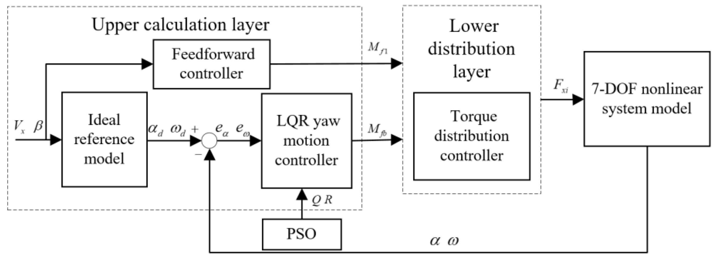
3.2. Variable Parameter LQR(VLQR) Yaw Motion Controller

The controller is designed in layers. The sideslip angle and yaw velocity characterizing the vehicle state are used as control variables. The LQR algorithm is used to solve for the direct yaw moment applicable to the vehicle. The PSO algorithm optimizes the parameters in the LQR to improve the controller control in the upper yaw torque calculation layer. In the lower torque distribution layer, the principle of minimum tire utilization is used to distribute the vehicle drive forces and additional yaw moments. The detailed process is shown in Figure 5.

Optimal control theory can be achieved under a certain model. It is reasonable to use the LQR optimal control theory to design the yaw moment feedback controller, considering the characteristics of the articulated vehicle. The vehicle condition tends to the target value with feedback compensation. The error equation between the real and desired values of the vehicle can be obtained from the 7 DOF nonlinear vehicle model with the desired state space equation:

$$e=X-X_{df}=\left(\begin{array}{c}\alpha -{\alpha }_{df}\\ \omega -{\omega }_{df}\end{array}\right)$$

(25)

where$X$is the sideslip angle and yaw velocity from the 7 DOF nonlinear vehicle model,$\mathrm{and} X_{df}$is the sideslip angle and yaw velocity from the desired state space equation.

For the derivative of the error, we can ignore higher-order and interference terms. The error deviation equation can be obtained as follows:

$$\dot{e}=A_{1}e+A_4{M}_{fb}$$

(26)

It is not desirable to introduce excessive feedback control while reducing the error. Therefore, it is necessary to limit the direct yaw moment of the feedback. The controller performance metric needs to be established to ensure that the LQR controller obtains the optimal solution. The design optimization objective function is as follows:

$$J={{\displaystyle \int }}_0^{\infty }\left[e^{T}Qe+M_{fb}^{T}R{M}_{fb}\right]dt$$

(27)

The optimal yaw moment is obtained when the minimum value of$J$is obtained, where $Q=\left[\begin{array}{cc}{q}_{\alpha }& 0\\ 0& q_w\end{array}\right],R=\left[r_{fb}\right]$. They are, respectively, the weighting matrices of the sideslip angle and yaw velocity in the LQR controller.$Q$is a semi-positive definite matrix, and $R$is a positive definite matrix. $q_{\alpha }$indicates the weight of the control system for the error between the sideslip angle and the desired value.$q_w$indicates the weight of the error between the angular velocity and the desired value. $r_{fb }$ indicates the degree of limitation on the yaw moment.

The standard linear quadratic (LQR) problem can be solved by establishing the infinite time optimal control Riccati equation.

$$PA+A^{T}P-PE{R}^{-1}{E}^{T}P+Q=0$$

(28)

We can solve the Riccati equation to obtain the state feedback gain matrix based on the LQR method.

$$G_{fb}=-R^{-1}{E}^{T}P$$

(29)

The direct yaw moment feedback torque is as follows:

$$M_{fb}=G_{fb}e=-g_1{e}_{\alpha }-g_1{e}_{\omega }$$

(30)

From the LQR algorithm deduction process and the optimal control law, we learn that the control effect of the controller depends entirely on the choice of parameters in the matrices Q and R. However, there is no analytical method for selecting parameters in the matrices. The selection of the parameters is different when the control and the optimization objectives are different.

Therefore, researchers often rely on subjective experience to select the parameters in the matrix and use extensive testing and simulation analysis to select the set of parameters with better control. This can consume a lot of time and effort, and in many cases, the parameters can only be adjusted qualitatively. The chosen matrix parameters are not guaranteed to obtain the optimal performance of the controller. Therefore, when selecting the matrix parameters, the “optimal matrix parameters” of the LQR controller for an articulated vehicle driving in a straight line at high speed are determined by the PSO algorithm according to the law of vehicle stability control.

3.3. Optimization of VLQR Controller Based on PSO

The particle swarm optimization (PSO) algorithm is a group collaboration stochastic search algorithm simulating birds’ foraging behavior. PSO is an ergodic optimization method, and the particle follows the optimal particle in a certain space to search for the optimal value iteratively. The position and velocity of the ith particle are denoted by $X_i$ and $V_i$, respectively. The fitness value of each particle is calculated by the objective optimization function. In each iteration, the particle updates itself by following two optimal results; one is the optimal result found by the particle itself, i.e., the individual optimum, and the other is the optimal result currently found by the whole population, i.e., the global optimum. The updated equations for the velocity and position of each particle are as follows:

$$\begin{array}{l}{v}_{i,j}\left(t+1\right)=w{v}_{i,j}\left(t\right)+c_1{r}_1\left[p_{i,j}-x_{i,j}\left(t\right)\right]+c_2{r}_2\left[p_{g,j}-x_{i,j}\left(t\right)\right]\\ x_{i,j}\left(t+1\right)=x_{i,j}\left(t\right)+v_{i,j}\left(t+1\right),j=1,2,\cdots ,d\end{array}$$

(31)

where$t$is the current iteration number$, w$is the inertia weight factor$, c_1$and $c_2$ are the positive learning factors$, and r_1$ and$r_2$are random numbers within$\left[0,1\right]$.

The particle swarm search space is three-dimensional when front-based or rear-based control is used. The front-based control parameters are$q_{\alpha f}$,$q_{wf}$,$\mathrm{and} r_{fbf}$, and the rear-based control parameters are$q_{\alpha r}$,$q_{wr}$, and $r_{fbr}$. The particle swarm search space is six-dimensional when the front and rear integrated control are ($q_{\alpha f}$,$q_{wf}$,$r_{fbf}$,$q_{\alpha r}$,$q_{wr}$,$r_{fbr}$). After generating the initial particle swarm, assigning the LQR control parameters, calculating the feedback gain, invoking the vehicle dynamics model, calculating the fitness, seeking and updating, and verifying the termination condition, the optimal LQR control parameters are eventually obtained. The specific process is shown in Figure 6.

The fitness function is the basic element of PSO. According to the characteristics of the articulated vehicle and the working conditions, considering the relationship between frequency and time domain, the sum of integrated time and absolute error (ITAE) of the sideslip angle and yaw velocity is selected as the fitness function to improve the response characteristics of the vehicle. It is expressed as:

$$\min T={{\displaystyle \int }}_0^{T}t\left|e_{\beta }\left(t\right)\right|\mathrm{dt}+{{\displaystyle \int }}_0^{T}t\left|e_{\omega }\left(t\right)\right|\mathrm{dt}$$

(32)

3.4. The Lower Torque Distribution Layer

The yaw moment generated by the PSO-LQR controller needs to be achieved by controlling the articulated vehicle with each wheel’s driving force. Due to the articulated configuration, the additional yaw moment of the front and rear vehicles can only be achieved by the tires on the respective vehicle. According to the friction ellipse principle of tires, the sum of the utilization rate of the four tires should be minimized for a high stability margin of the vehicle, as shown in Equation (33). The drive torque can be distributed according to the wheel load so that the vehicle has a large lateral traction margin to improve vehicle safety.

$$\min J={\displaystyle \sum }_{i=j}^4{C}_j\frac{F_{xj}^2+F_{yj}^2}{{\mu }^2{F}_{zj}^2}$$

(33)

Here, $C_j$is the weight factor of each wheel. Since the differences between the drive motors of each wheel are not considered, the weighting factor of each wheel $C_j$ is set to 1. When the vehicle is driving, it is more difficult to obtain the lateral force of the tire compared with the longitudinal force of the tire, and the lateral force of the tire and the vertical load of each wheel do not change suddenly. Therefore, Equation (33) can be simplified as follows:

$$\min J={\displaystyle \sum }_{j=1}^4{C}_j\frac{F_{xj}^2}{{\mu }^2{F}_{zj}^2}$$

(34)

The total longitudinal drive force of the articulated vehicle should be first satisfied when the yaw moment is distributed. In addition, the longitudinal force is limited by the road adhesion conditions, and the driving force of each wheel cannot exceed the maximum driving force that each drive motor can provide or the maximum friction between the tires and the ground. Thus, the parameters in the target equation should satisfy the following constraints:

$$\{\begin{array}{l}{F}_{x1}+F_{x2}+F_{x3}+F_{x4}=F_d\\ B\left(F_{x1}-F_{x2}\right)=M_1\\ B\left(F_{x3}-F_{x4}\right)=M_2\\ -\mu F_{zj}\le F_{xj}\le \min \left(\mu F_{zj},F_{max}\right)\end{array}$$

(35)

where $F_d$is the total required longitudinal drive force.

When the vehicle performs stability control with the front-based or rear-based control, the other vehicle is without a yaw moment. However, when the vehicle performs stability control with front and rear integrated control, both front and rear vehicles apply yaw moment. Compared with the front-based or rear-based control individually, more units are controlled, and the front and rear integrated control effects are most likely better in theory.

4. Simulation Analysis

To comprehensively analyze the effectiveness and characteristics of the control system, the stability controller constructed in Section 3 is simulated at 5 m/s under low-speed conditions and 15 m/s under high-speed conditions. Simulation and comparative analysis of the LQR controller with unoptimized parameters (later denoted by LQR) and the optimized parameters of PSO (later denoted by PSO-LQR) are conducted under four conditions: uncontrolled, front-based control, rear-based control, and front and rear integrated control. The simulation and analysis validate the effectiveness and advantages of LQR control methods and PSO optimization. The parameters in the model are shown in

Table 1. Parameters of the vehicle dynamics model.

Parameters	Values	Parameters	Values
$m_1$	$6980 \mathrm{kg}$	$\mu$	$0.8$
m2	$9767 \mathrm{kg}$	$reff$	$0.875 \mathrm{m}$
$L_1$	$0.25 \mathrm{m}$	$C_{\sigma }$	$2\times {10}^5 \mathrm{N}/\mathrm{m}$
$L_2$	1.35 m	$C_{\alpha }$	$5\times {10}^4 \mathrm{N}/\mathrm{rad}$
$L_3$	$0.2 \mathrm{m}$	$R$	$0.45 \mathrm{m}$
$L_4$	$1.459 \mathrm{m}$	$r$	$0.55 \mathrm{m}$
$B$	$1.15 \mathrm{m}$	$A_1$	$0.002826{ \mathrm{m}}^2$
$I_1$	32,977 ${ \mathrm{kgm}}^2$	$A_2$	$0.002112{ \mathrm{m}}^2$
I2	13,228 ${ \mathrm{kgm}}^2$	$V_0$	$0.0015{ \mathrm{m}}^3$

.

4.1. Comparative Analysis of Uncontrolled Conditions and LQR Control

This subsection compares the simulation of the uncontrolled condition and various LQR controllers for articulated vehicles at 5 m/s and 15 m/s to initially verify the validity of the controller. After debugging, the LQR controller parameters are taken as follows: front-based control ($q_{\alpha f}={10}^6$, $q_{wf}={10}^5$, $r_{fbf}={10}^{-4}$), rear-based control ($q_{ar}={10}^5$, $q_{wr}={10}^3$, $r_{fbr}={10}^{-6}$), and front and rear integrated control ($q_{\alpha f}={10}^6$, $q_{wf}={10}^4$, $r_{fbf}={10}^{-6}$, $q_{\alpha r}={10}^6$, $q_{wr}={10}^2$, $r_{fbr}={10}^{-6}$). With the articulated vehicle traveling at 5 m/s, the articulated angle is shown in Figure 7, and the other parameters of the articulated vehicle without control and under various base controls are shown in Figure 8.

From the simulation results, it is obvious that the LQR controller, whether it is front-based control, rear-based control, or front and rear-integrated control, has a more obvious control effect compared to the uncontrolled condition. They can limit the articulated angle’s amplitude and accelerate the convergence speed. However, the front and rear integrated control effects are significantly better than the front-based control and the rear-based control both in terms of oscillation amplitude and convergence speed. The rear-based control is intermediate, and the front-based control is the least effective.

The angular velocity of the front and rear vehicle body is similar to the articulated angle, and all three controls limit the amplitude of oscillation and accelerate the convergence speed. However, the front and rear integrated control effects are the best, and front-based control is the worst. In terms of the front and rear vehicle body lateral acceleration, front-body lateral acceleration is slightly greater than that of rear-body acceleration. Although the front and rear integrated control amplitude is the largest, the convergence speed is the fastest. Because of the relationship between acceleration and force, this indicates that the front and rear integrated control response is faster, and the yaw moment is larger, so it has a better convergence speed. Therefore, when the articulated vehicle is driving at 5 m/s, all three controls have a good suppression effect on snaking oscillation. However, the front and rear integrated control are the best, rear-based control is the second best, and front-based control is the worst.

With the articulated vehicle driving at 15 m/s, the articulated angle is shown in Figure 9, and the other parameters of the articulated vehicle without control and under various base controls are shown in Figure 10.

All three controls have significant control effects. In the uncontrolled condition, the vehicle’s articulated angle is in the convergence state, but the convergence speed is slow, and the mean amplitude centerline gradually deviates from zero. The angular velocity of the front and rear vehicle body, the lateral acceleration, and the lateral velocity gradually increases. At this point, the vehicle appears to be running off course. After control, all vehicle parameters can be quickly converged, i.e., the snaking oscillation can be better suppressed, and the run-out phenomenon can be suppressed. These results are still based on the best-combined control of the front and rear body, followed by that of the rear body and that of the front body, which is the worst. Similar to at lower speeds, front and rear-integrated control is still obviously best, rear-based control is the second best, and front-based control is the worst. However, the effect of rear-based control is not as advantageous as front-based control at low speeds. Especially at convergence speeds, the front-base convergence speed is slightly better.

4.2. Comparative Analysis of LQR and PSO-LQR

In this section, the PSO effect is verified by comparing the artificially rectified LQR parameter controller with the PSO-LQR controller under the three controls: front-based control, rear-based control, and front and rear integrated control. Due to the space limitations, this section analyzes the articulated vehicle based on three types of control when it is driving at 15 m/s.

4.2.1. Comparative Analysis of Front-Based Control

To improve the algorithm search efficiency, according to experience and simulation, the initial population number is assumed to be 50, and the iteration number is assumed to be 80. The search space is limited to a certain range. The optimal value is finally found, and the optimized control parameters are shown in

Table 2. Front-based control search range and optimization results.

Name	${\mathit{q}}_{\mathit{\alpha }\mathit{f}}$	${\mathit{q}}_{\mathit{w}\mathit{f}}$	${\mathit{r}}_{\mathit{f}\mathit{b}\mathit{f}}$
Range	$\left[{10}^3,{10}^7\right]$	$\left[{10}^2,{10}^6\right]$	$\left[{10}^{-6},1\right]$
Optimal result	$7.27\times {10}^5$	$1.01\times {10}^5$	$1.75\times {10}^{-5}$

. The articulated angle is shown in Figure 11, and the other parameters after controlling the LQR and PSO-LQR are shown in Figure 12.

According to the simulation results, the PSO-LQR controller has a better suppression effect on the snaking oscillation both in amplitude and convergence speed. For the angular velocity, lateral velocity, and lateral acceleration of the front and rear vehicle body, the PSO-LQR controller still works better. Although the amplitudes of the front and rear vehicle body accelerations are larger under PSO-LQR control at the initial moment, the subsequent convergence time is shorter. This also indicates that the response is fast and the feedback control is better. The PSO algorithm’s effectiveness and the vehicle stability improvement after optimization are demonstrated.

4.2.2. Comparative Analysis of Rear-Based Control

The initial population and iteration numbers are the same as those of front-based control. The rear-based control search range and optimized control parameters are shown in

Table 3. Rear-based control search range and optimization results.

Name	${\mathit{q}}_{\mathit{\alpha }\mathit{r}}$	${\mathit{q}}_{\mathit{w}\mathit{r}}$	${\mathit{r}}_{\mathit{f}\mathit{b}\mathit{r}}$
Range	$\left[{10}^3,{10}^6\right]$	$\left[{10}^2,{10}^5\right]$	$\left[{10}^{-7},1\right]$
Optimal result	$5.39\times {10}^4$	$1.52\times {10}^4$	$8.52\times {10}^{-7}$

. The articulated angle is shown in Figure 13, and the other parameters after controlling the LQR and PSO-LQR are shown in Figure 14.

4.2.3. Comparative Analysis of Front and Rear Integrated Control

The search range and optimized parameters are shown in

Table 4. Front and rear integrated control search range and optimization results.

Name	${\mathit{q}}_{\mathit{\alpha }\mathit{f}}$	${\mathit{q}}_{\mathit{w}\mathit{f}}$	${\mathit{r}}_{\mathit{f}\mathit{b}\mathit{f}}$	${\mathit{q}}_{\mathit{\alpha }\mathit{r}}$	${\mathit{q}}_{\mathit{w}\mathit{r}}$	${\mathit{r}}_{\mathit{f}\mathit{b}\mathit{r}}$
Range	$\left[{10}^3,{10}^7\right]$	$\left[{10}^{-9},{10}^{-6}\right]$	$\left[{10}^{-9},{10}^{-6}\right]$	$\left[{10}^3,{10}^5\right]$	$\left[{10}^2,{10}^4\right]$	$\left[{10}^{-9},{10}^{-6}\right]$
Optimal result	$4.15\times {10}^4$	$1.05\times {10}^{-9}$	$1.59\times {10}^{-9}$	$3.69\times {10}^4$	$8.47\times {10}^2$	$1.31\times {10}^{-9}$

. The articulated angle is shown in Figure 15, and the parameters in integrated front and rear body control of LQR and PSO-LQR are shown in Figure 16.

According to the simulation results, the overall control effect of the PSO-LQR controller is better. Particularly, the optimization effect on the control of the articulated angle is obvious. The oscillation amplitude is greatly reduced, and the convergence speed is accelerated. The optimization effect on the amplitude of the front and rear vehicle angular velocity is not obvious, but the convergence speed is accelerated. The oscillation amplitude is greater in the lateral acceleration of the front and rear car bodies while the convergence speed is increased. Overall, the LQR controller parameters optimized by the PSO algorithm have a better control effect and can improve the suppression effect of the articulated vehicle snaking in the time and frequency domains to improve vehicle stability.

The articulated angle is shown in Figure 17, and the other parameters of the articulated vehicle under three PSO-LQR controls at 15 m/s are shown in Figure 18.

After PSO algorithm optimization, the effect of the snaking oscillation suppression based on front and rear integrated control for articulated vehicles is still the best, and the advantage is obvious. Rear-based control is significantly more effective than front-based control. Overall, rear-based control is better than front-based control for snaking oscillation suppression. The advantage is greater than when the LQR controller parameters are not optimized by PSO. Rear-based control has better oscillation amplitude suppression, and although the convergence speed is slowed down, the convergence process is relatively smooth. In terms of the front and rear vehicle angular velocity, rear-based control is also better than front-based control, with no significant difference in the convergence speed, and the amplitude decreases significantly and changes smoothly. However, in terms of the front vehicle lateral velocity, front body-based control is better.

The articulated vehicle driving force of each tire under the three PSO-LQR controls is shown in Figure 19. The tire force based on the front and rear integrated control at the moment of snaking oscillation emergence shows the greatest amplitude. However, the oscillation frequency during the convergence is the highest, and the convergence speed is the fastest. Since force is the reason for changing the motion state, front and rear integrated control is the most effective for articulated vehicle snaking oscillation suppression control. Compared with rear-based control, front-based control has a slightly faster convergence rate and higher oscillation frequency because the tires have rolling friction with the ground, and the front and rear vehicle weights and center of gravity positions are different. Therefore, the driving force of each tire is not zero, and the driving force of the tires of the front and rear vehicles are different during articulated vehicle stable driving after suppressing the snaking oscillation.

5. Conclusions

The articulated vehicle 7 DOF nonlinear system model and the three control desirable reference models were obtained herein. The PSO-LQR upper-level yaw torque controller and the lower torque distribution layer for snaking oscillation yaw motion control were established.

The effectiveness of the front-based, rear-based, and front and rear-integrated LQR controllers was initially verified by comparing them with uncontrolled conditions at different speeds. All three controls can limit the articulated angle oscillation amplitude and convergence speed. The three controls can also suppress the snaking oscillation at higher speeds while ensuring the straightness of vehicle driving. The front and rear integrated control effects are significantly better than the front-based and rear-based control. The rear-based control effect is medium, and the front-based control effect is the worst.

PSO optimizes the parameters in the LQR controller, and the control effect of the three controllers after parameter optimization is improved both in oscillation amplitude and convergence speed. In contrast, the front and rear integrated control effects improved the most after parameter optimization. After parameter optimization, comparing the control effect under the three controls shows that the front and rear integrated control effect is obviously the best, followed by rear-based control, and the front-based control effect is the worst. The front and rear integrated control tire forces have the largest amplitude, highest oscillation frequency, and fastest convergence rate. In conclusion, the proposed layered stability controller and the PSO algorithm to optimize LQR controller parameters for snaking oscillation control are effective.

6. Discussion

This paper focuses on the three control modes and compares LQR and PSO-LQR control for articulated vehicles’ snaking oscillation control. The proposed front and rear integrated control and PSO-LQR can substantially improve the articulated vehicles’ snaking oscillation suppression effect. The control method proposed in the study is under the condition that the parameters of articulated vehicles are known and invariable. However, due to the inherent characteristics of PSO and LQR optimization algorithms and the performance limitations of controller hardware, the method proposed in the study does not allow PSO to optimize the parameters in the LQR controller in real time under different operating conditions and variable vehicle parameters. Therefore, the real-time optimization of the articulated vehicles’ snaking suppression with variable body parameters and operating conditions should be the focus of subsequent research.

References

1. Lashgarian Azad, N.; Khajepour, A.; Mcphee, J. Robust state feedback stabilization of articulated steer vehicles. Veh. Syst. Dyn. 2007, 45, 249–275. [Google Scholar] [CrossRef]
2. Dudziński, P.; Skurjat, A. Directional dynamics problems of an articulated frame steer wheeled vehicles. J. KONES 2012, 19, 89–98. [Google Scholar] [CrossRef]
3. Crolla, D. The steering behaviour of articulated body steer vehicles. In Proceedings of the Road Vehicle Handling, I Mech E Conference Publications 1983-5. Sponsored by Automobile Division of the Institution of Mechanical Engineers under patronage of Federation Internationale des Societies d’Ingenieurs des Techniques de l’Automobile (FISITA), Motor Industry Research Association, Nuneaton, UK, 24–26 May 1983. [Google Scholar]
4. Azad, N.L.; Khajepour, A.; McPhee, J. Effects of locking differentials on the snaking behaviour of articulated steer vehicles. Int. J. Veh. Syst. Model. Test. 2007, 2, 101. [Google Scholar] [CrossRef]
5. Horton, D.N.L.; Crolla, D.A. Theoretical Analysis of the Steering Behaviour of Articulated Frame Steer Vehicles. Veh. Syst. Dyn. 1986, 15, 211–234. [Google Scholar] [CrossRef]
6. He, Y.; Khajepour, A.; McPhee, J.; Wang, X. Dynamic modelling and stability analysis of articulated frame steer vehicles. Int. J. Heavy Veh. Syst. 2005, 12, 28. [Google Scholar] [CrossRef]
7. Gao, Y.; Shen, Y.; Yang, Y.; Zhang, W.; Güvenç, L. Modelling, verification and analysis of articulated steer vehicles and a new way to eliminate jack-knife and snaking behaviour. Int. J. Heavy Veh. Syst. 2019, 26, 375. [Google Scholar] [CrossRef]
8. Azad, N.L.; Khajepour, A.; McPhee, J. A survey of stability enhancement strategies for articulated steer vehicles. Int. J. Heavy Veh. Syst. 2009, 16, 26. [Google Scholar] [CrossRef]
9. Azad, N.L.; Khajepour, A.; Mcphee, J. Stability Control of Articulated Steer Vehicles by Passive and Active Steering Systems. In Proceedings of the 2005 SAE Commercial Vehicle Engineering Conference, Rosemont, IL, USA, 1–3 November 2005. [Google Scholar] [CrossRef]
10. Xu, T.; Ji, X.; Shen, Y. A novel assist-steering method with direct yaw moment for distributed-drive articulated heavy vehicle. Proc. Inst. Mech. Eng. Part K J. Multi-Body Dyn. 2020, 234, 214–224. [Google Scholar] [CrossRef]
11. Ono, E.; Hattori, Y.; Muragishi, Y.; Koibuchi, K. Vehicle dynamics integrated control for four-wheel-distributed steering and four-wheel-distributed traction/braking systems. Veh. Syst. Dyn. 2006, 44, 139–151. [Google Scholar] [CrossRef]
12. He, P.; Hori, Y. Optimum traction force distribution for stability improvement of 4WD EV in critical driving condition. In Proceedings of the 9th IEEE International Workshop on Advanced Motion Control, Istanbul, Turkey, 27–29 March 2006. [Google Scholar]
13. Bharali, J.; Buragohain, M. Design and performance analysis of Fuzzy LQR; Fuzzy PID and LQR controller for active suspension system using 3 Degree of Freedom quarter car model. In Proceedings of the 2016 IEEE 1st International Conference on Power Electronics, Intelligent Control and Energy Systems (ICPEICES), Delhi, India, 4–6 July 2016; pp. 1–6. [Google Scholar]
14. Gao, L.; Jin, L.; Wang, F.; Zheng, Y.; Li, K. Genetic algorithm–based varying parameter linear quadratic regulator control for four-wheel independent steering vehicle. Adv. Mech. Eng. 2015, 7, 168781401561863. [Google Scholar] [CrossRef] [Green Version]
15. Nie, Z.; Gao, J.; Zhang, K. Integrated control strategy for articulated heavy vehicles based on a linear model with real-time parameters. Int. J. Heavy Veh. Syst. 2019, 26, 432. [Google Scholar] [CrossRef]
16. Esmaeili, N.; Kazemi, R.; Tabatabaei Oreh, S.H. An adaptive sliding mode controller for the lateral control of articulated long vehicles. Proc. Inst. Mech. Eng. Part K J. Multi-Body Dyn. 2019, 233, 487–515. [Google Scholar] [CrossRef]
17. Jiang, Z.; Xiao, B. LQR optimal control research for four-wheel steering forklift based-on state feedback. J. Mech. Sci. Technol. 2018, 32, 2789–2801. [Google Scholar] [CrossRef]
18. Azad, N.L. Dynamic Modelling and Stability Controller Development for Articulated Steer Vehicles. Ph.D. Thesis., University of Waterloo, Waterloo, ON, Canada, 2006; p. 196. Available online: http://hdl.handle.net/10012/2633 (accessed on 26 October 2022).
19. Wang, W.; Fan, J.; Xiong, R.; Sun, F. Lateral stability control of four wheels independently drive articulated electric vehicle. In Proceedings of the 2016 IEEE Transportation Electrification Conference and Expo (ITEC), Dearborn, MI, USA, 27–29 June 2016; pp. 1–5. [Google Scholar]
20. Abroshan, M.; Hajiloo, R.; Hashemi, E.; Khajepour, A. Model predictive-based tractor-trailer stabilisation using differential braking with experimental verification. Veh. Syst. Dyn. 2021, 59, 1190–1213. [Google Scholar] [CrossRef]
21. Dudziński, P.; Skurjat, A. System for Improving Directional Stability for Articulated Vehicles. In Proceedings of the Computational Technologies in Engineering (TKI’2018): Proceedings of the 15th Conference on Computational Technologies in Engineering, Jora Wielka, Poland, 16–19 December 2018; p. 020084. [Google Scholar] [CrossRef]
22. Lin, C.; Cheng, X. A Traction Control Strategy with an Efficiency Model in a Distributed Driving Electric Vehicle. Sci. World J. 2014, 2014, 261085. [Google Scholar] [CrossRef] [PubMed] [Green Version]
23. Gao, Y.; Shen, Y.; Xu, T.; Zhang, W.; Guvenc, L. Oscillatory Yaw Motion Control for Hydraulic Power Steering Articulated Vehicles Considering the Influence of Varying Bulk Modulus. IEEE Trans. Control Syst. Technol. 2019, 27, 1284–1292. [Google Scholar] [CrossRef]
24. Xu, T.; Ji, X.; Liu, Y.; Liu, Y. Differential Drive Based Yaw Stabilization Using MPC for Distributed-Drive Articulated Heavy Vehicle. IEEE Access 2020, 8, 104052–104062. [Google Scholar] [CrossRef]
Figure 1. Articulated vehicle dynamics model.
Actuators 11 00337 g001
Figure 2. Articulated vehicle vertical force analysis.
Actuators 11 00337 g002
Figure 3. Hydraulic steering system model.
Actuators 11 00337 g003
Figure 4. The front-based control 3 DOF reference model.
Actuators 11 00337 g004
Figure 5. The layered stability control schematic of the articulated vehicle.
Actuators 11 00337 g005
Figure 6. PSO optimization flow chart.
Actuators 11 00337 g006
Figure 7. Articulated angle.
Actuators 11 00337 g007
Figure 8. Simulation results: (a) Front body angular velocity; (b) Rear body angular velocity; (c) Front body lateral acceleration; (d) Rear body lateral acceleration; (e) Front body lateral velocity; (f) Rear body lateral velocity.
Actuators 11 00337 g008
Figure 9. Articulated angle.
Actuators 11 00337 g009
Figure 10. Simulation results: (a) Front body angular velocity; (b) Rear body angular velocity; (c) Front body lateral acceleration; (d) Rear body lateral acceleration; (e) Front body lateral velocity; (f) Rear body lateral velocity.
Actuators 11 00337 g010
Figure 11. Articulated angle.
Actuators 11 00337 g011
Figure 12. Simulation results: (a)Front body angular velocity; (b) Front body lateral acceleration; (c) Front body lateral velocity; (d) Rear body angular velocity; (e) Rear body lateral acceleration; (f) Rear body lateral velocity.
Actuators 11 00337 g012
Figure 13. Articulated angle.
Actuators 11 00337 g013
Figure 14. Simulation results: (a) Front body angular velocity; (b) Front body lateral acceleration; (c) Front body lateral velocity; (d) Rear body angular velocity; (e) Rear body lateral acceleration; (f) Rear body lateral velocity.
Actuators 11 00337 g014
Figure 15. Articulated angle.
Actuators 11 00337 g015
Figure 16. Simulation results: (a) Front body angular velocity; (b) Front body lateral acceleration; (c) Front body lateral velocity; (d) Rear body angular velocity; (e) Rear body lateral acceleration; (f) Rear body lateral velocity.
Actuators 11 00337 g016
Figure 17. Articulated angle.
Actuators 11 00337 g017
Figure 18. Simulation results: (a) Front body angular velocity; (b) Rear body angular velocity; (c) Front body lateral acceleration; (d) Rear body lateral acceleration; (e) Front body lateral velocity; (f) Rear body lateral velocity.
Actuators 11 00337 g018
Figure 19. Simulation results: (a) Each tire’s driving force under front-based control; (b) Each tire’s driving force under rear-based control; (c) Each tire’s driving force under the front and rear integrated control.
Actuators 11 00337 g019