
Direct Thrust Force Control of Primary Permanent Magnet Linear Motor Based on Improved Extended State Observer and Model-Free Adaptive Predictive Control


Abstract
:1. Introduction
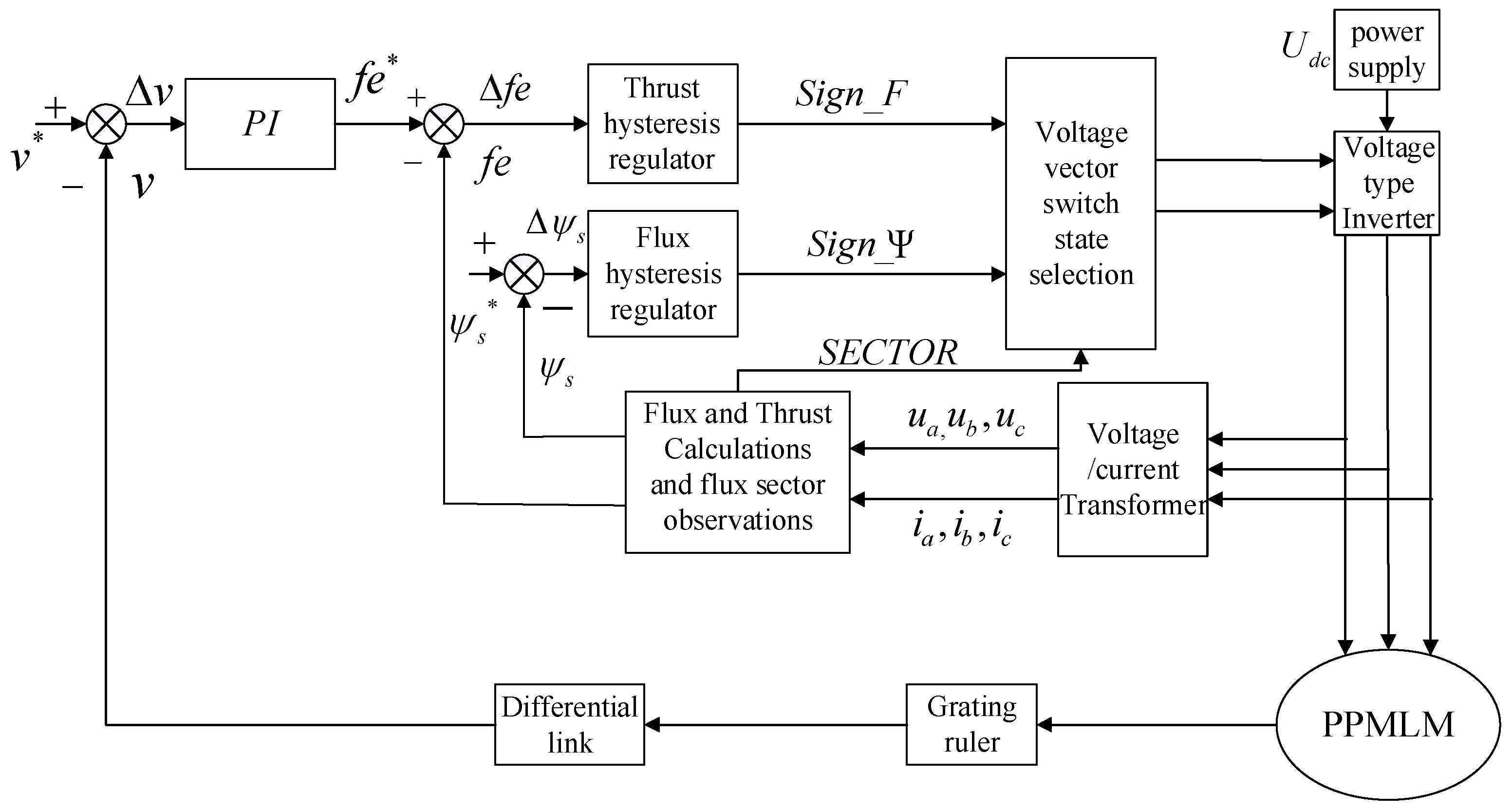
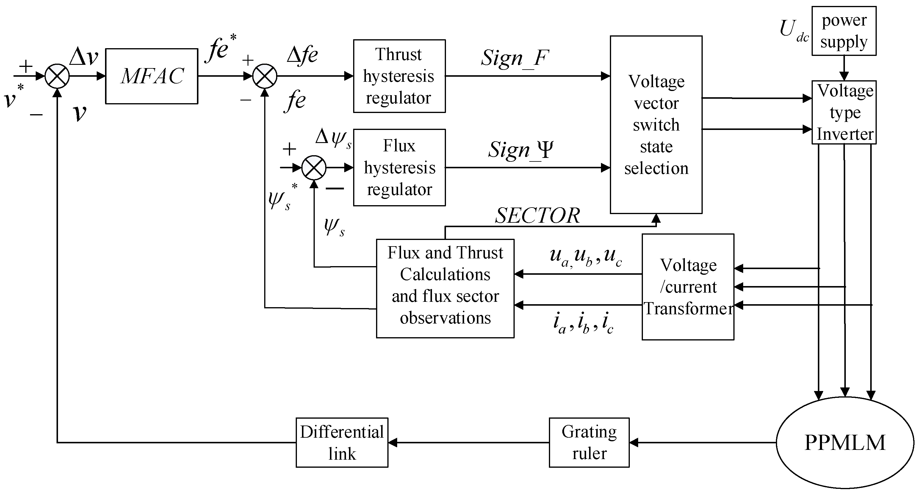
2. PPMLM DTFC System
3. Design of the MFAC Algorithm
3.1. Design of the Control Algorithm Based on CFDL−MFAC
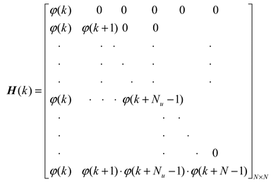
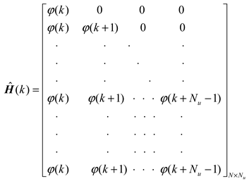
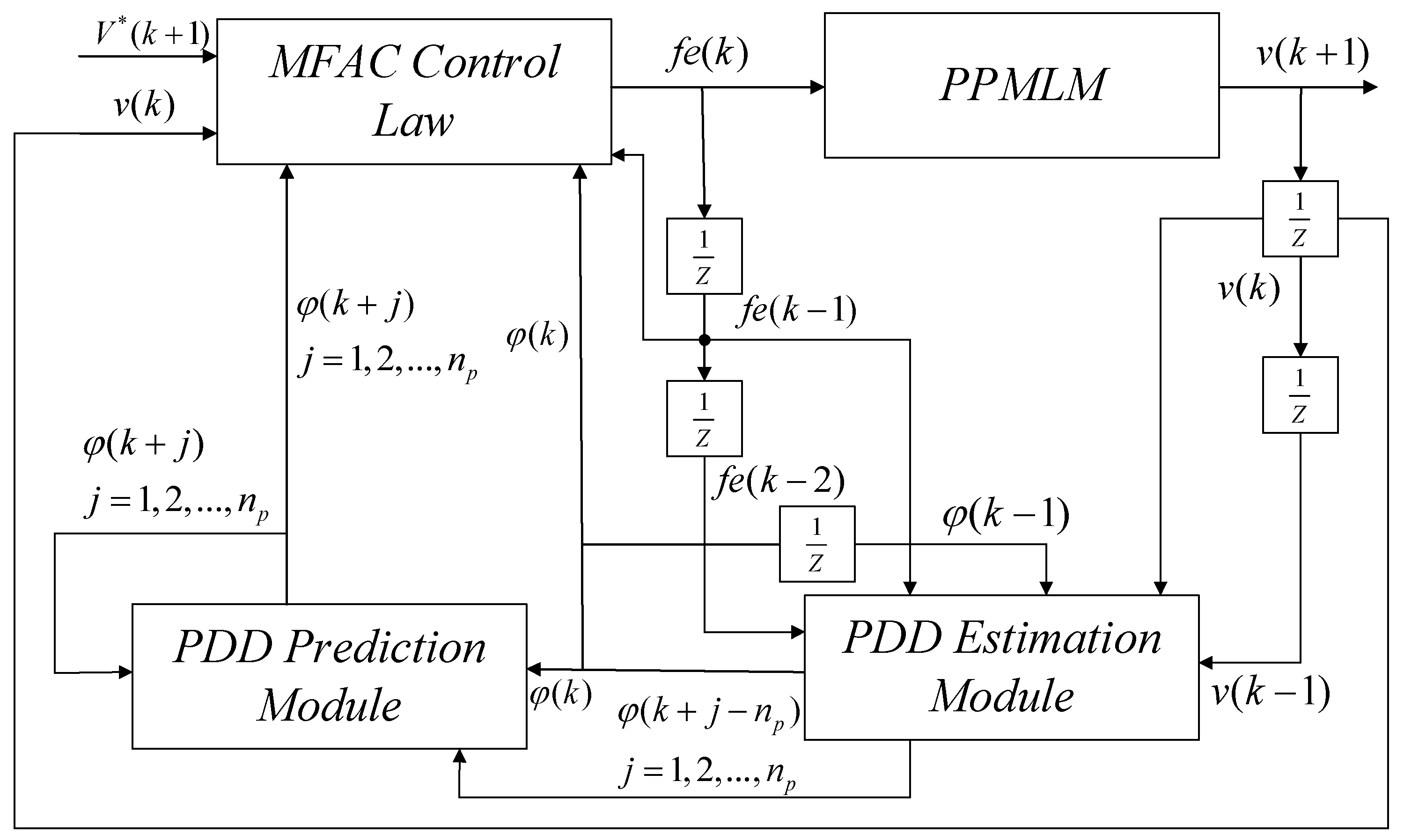
3.2. Design of the Control Algorithm Based on CFDL−MFAPC
 .
.
 .
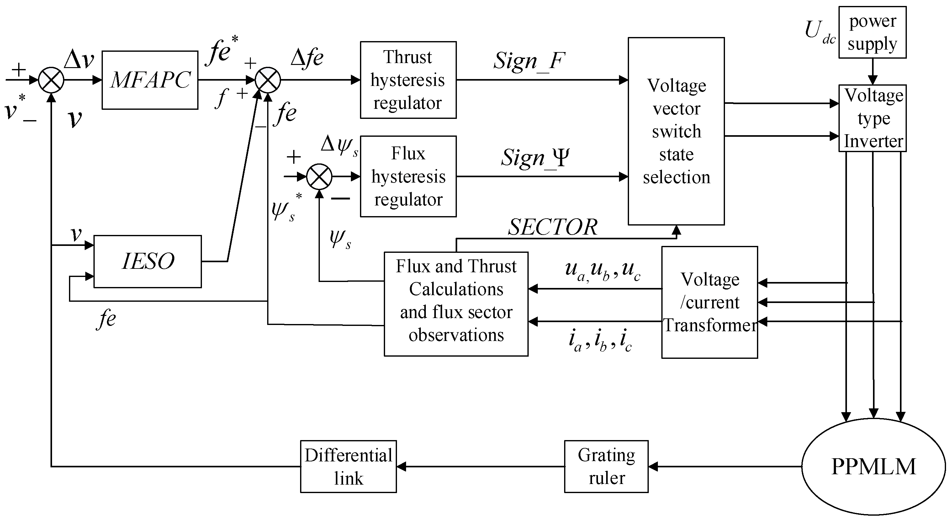
.3.3. Design of the Control Algorithm Based on IESO−CFDL−MFAPC
3.4. Closed-Loop Stability Proof of the PPMLM Direct Thrust Control System Based on IESO-CFDL-MFAPC
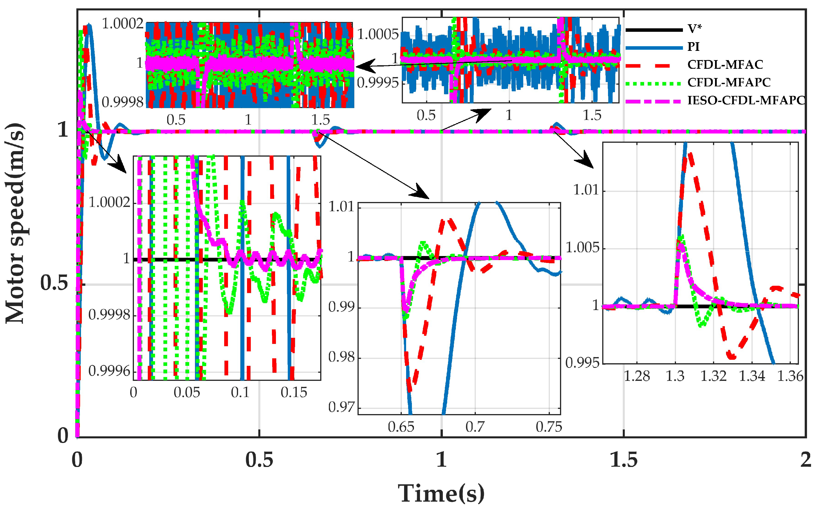
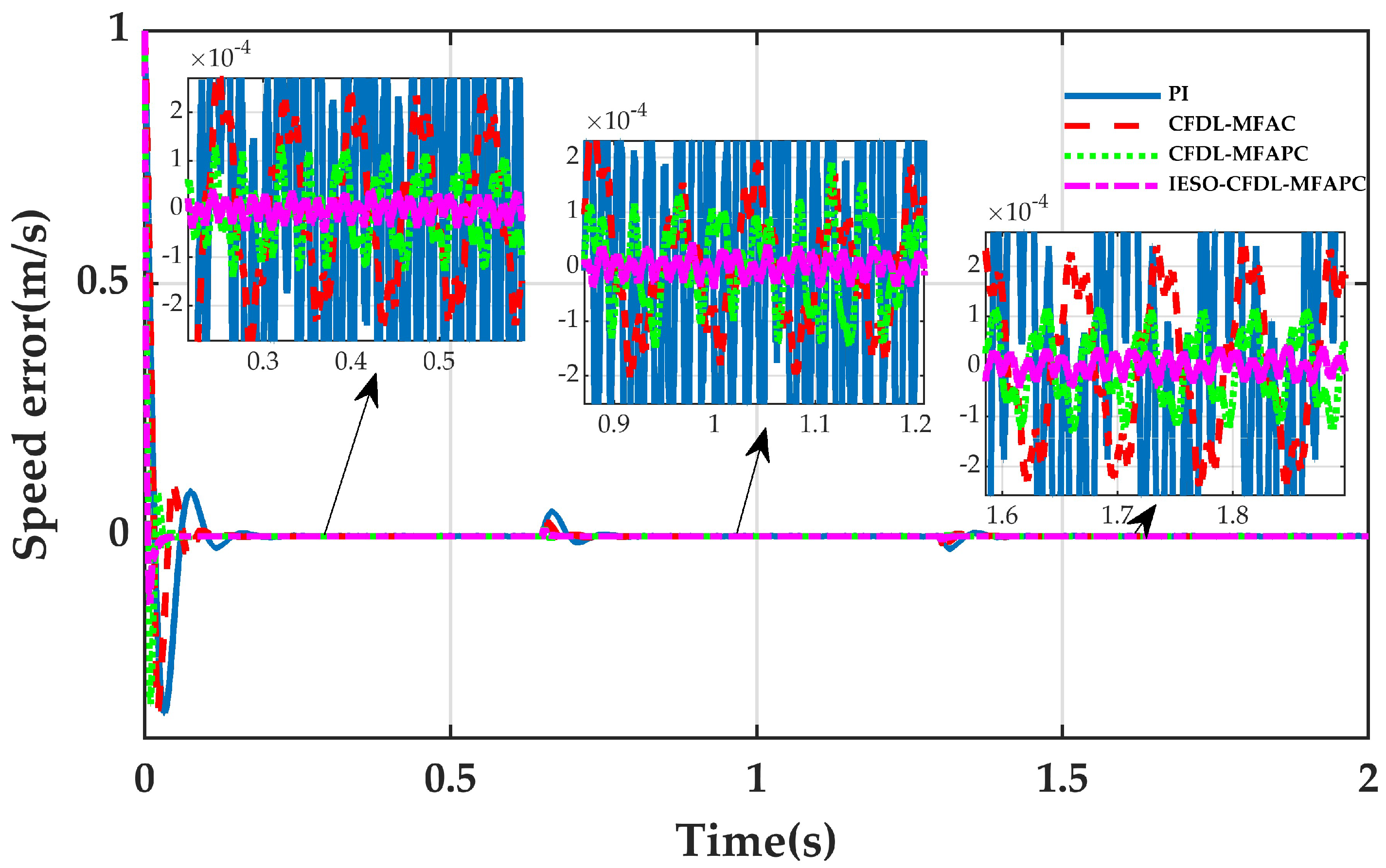
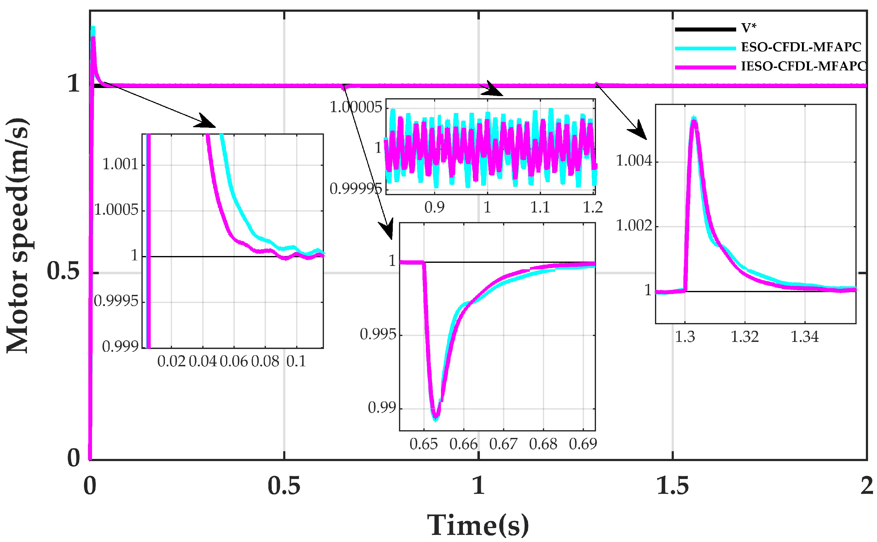
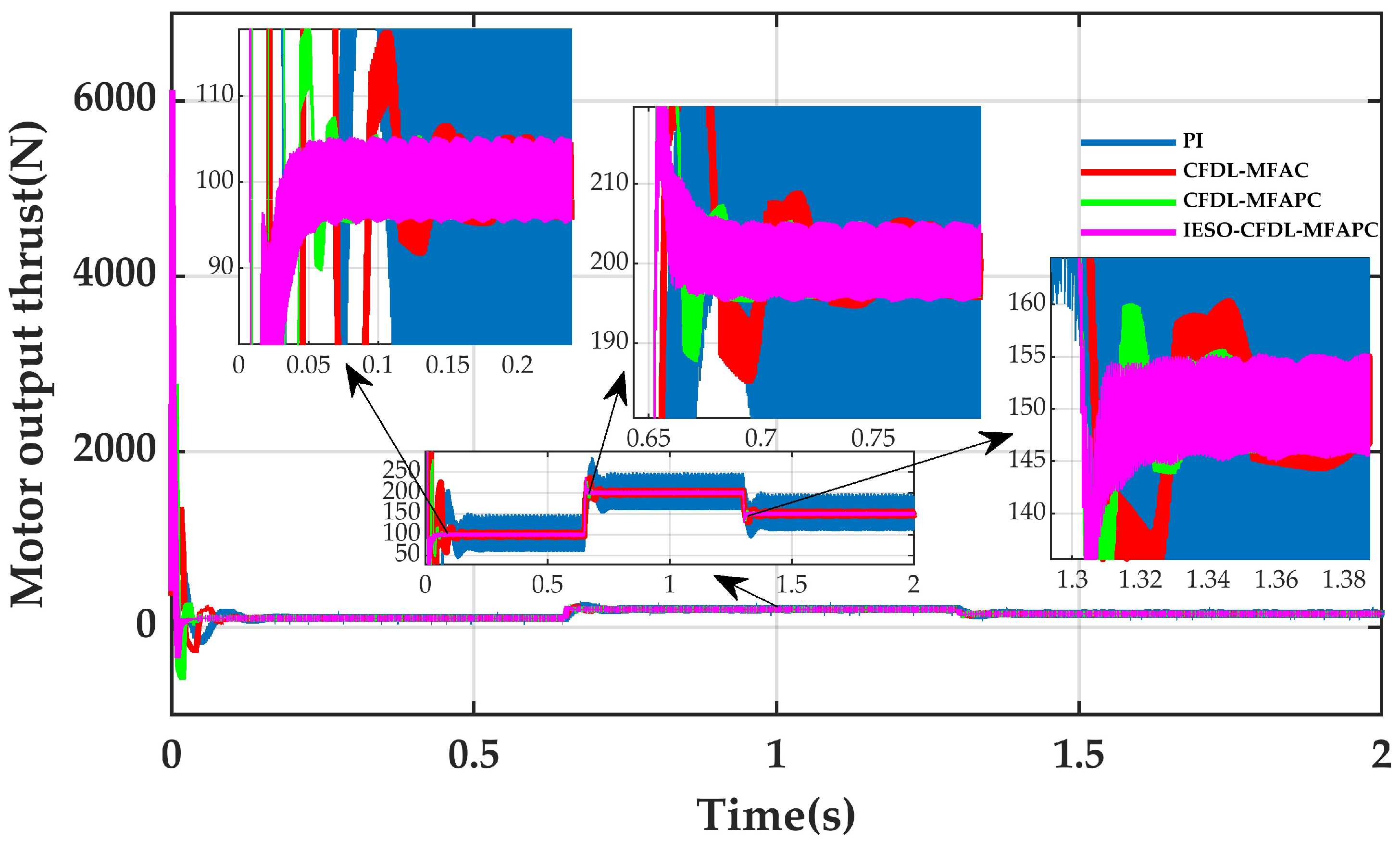
4. Simulation Verification
5. Conclusions
Author Contributions
Funding
Institutional Review Board Statement
Informed Consent Statement
Conflicts of Interest
References
- Lyu, G. Review of the Application and Key Technology in the Linear Motor for the Rail Transit. Proc. CSEE 2020, 40, 5665–5675. [Google Scholar]
- Huang, S.; Ching, T.W.; Li, W.; Deng, B. Overview of linear motors for Transportation applications. In Proceedings of the 2018 IEEE 27th International Symposium on Industrial Electronics (ISIE), Cairn, Australia, 13–15 June 2018; pp. 150–154. [Google Scholar]
- Boldea, I.; Tutelea, L.N.; Xu, W.; Marcello, P. Linear electric machines, drives, and MAGLEVs: An overview. IEEE Trans. Ind. Electron. 2018, 65, 7504–7515. [Google Scholar] [CrossRef]
- Wang, W.; Feng, Y.; Shi, Y.; Cheng, M.; Hua, W.; Wang, Z. Direct Thrust Force Control of Primary Permanent-Magnet Linear Motors with Single DC-Link Current Sensor for Subway Applications. IEEE Trans. Power Electron. 2019, 35, 1365–1376. [Google Scholar] [CrossRef]
- Wang, W.; Feng, Y.; Shi, Y.; Cheng, M.; Hua, W.; Wang, Z. Fault-tolerant control of primary permanent-magnet linear motors with single-phase current sensor for subway applications. IEEE Trans. Power Electron. 2019, 34, 10546–10556. [Google Scholar] [CrossRef]
- Karimi, H.; Vaez-Zadeh, S.; Salmasi, F.R. Combined vector and direct thrust control of linear induction motors with end effect compensation. IEEE Trans. Energy Convers. 2015, 31, 196–205. [Google Scholar] [CrossRef]
- Zhao, X.; Jin, Y.; Wang, L. Adaptive RBFNN backstepping control for PMLSM servo system. Electr. Mach. Control 2020, 24, 149–157. [Google Scholar]
- Hu, Y.; Wang, H.; He, S.; Zheng, J.; Ping, Z.; Shao, K.; Cao, Z.; Man, Z. Adaptive Tracking Control of an Electronic Throttle Valve Based on Recursive Terminal Sliding Mode. IEEE Trans. Veh. Technol. 2021, 70, 251–262. [Google Scholar] [CrossRef]
- Zhang, J.; Wang, H.; Ma, M.; Yu, M.; Yazdani, A.; Chen, L. Active Front Steering-based Electronic Stability Control for Steer-by-Wire Vehicles via Terminal Sliding Mode and Extreme Learning Machine. IEEE Trans. Veh. Technol. 2020, 69, 14713–14726. [Google Scholar] [CrossRef]
- Jin, X.; Zhao, Y.; Wang, H.; Zhao, Z.; Dong, X. Adaptive fault-tolerant control of mobile robots with actuator faults and unknown parameters. IET Control Theory Appl. 2019, 13, 1665–1672. [Google Scholar] [CrossRef]
- Yeam, T.; Lee, D. Design of Sliding-Mode Speed Controller with Active Damping Control for Single-Inverter Dual-PMSM Drive Systems. IEEE Trans. Power Electron. 2021, 36, 5794–5801. [Google Scholar] [CrossRef]
- Zhao, X.; Liu, C.; Zhu, G. Adaptive nonlinear sliding mode control for permanent magnet linear synchronous motor. Electr. Mach. Control 2020, 24, 39–47. [Google Scholar]
- Zhao, X.; Zhao, J. Complementary Sliding Mode Variable Structure Control for Permanent Magnet Linear Synchronous Motor. Proc. CSEE 2015, 35, 2552–2557. [Google Scholar]
- Zhao, X.; Ji, X.; Wang, H. Time delay adaptive integral sliding mode control for permanent magnet linear synchronous motor. Electr. Mach. Control 2020, 24, 44–50. [Google Scholar]
- Chen, X.; Zhao, W.; Ji, J.; Tao, T.; Xue, R. Model Predictive Current Control of Double-Side Linear Vernier Permanent Magnet Machines Considering End Effect. Trans. China Electrotech. Soc. 2019, 34, 49–57. [Google Scholar]
- Li, Z.; An, J.; Xiao, Y.; Zhang, Q.; Sun, H. Design of Model Predictive Control System for Permanent Magnet Synchronous Linear Motor Based on Adaptive Observer. Trans. China Electrotech. Soc. 2021, 36, 1190–1200. [Google Scholar]
- Carlet, P.G.; Favato, A.; Bolognani, S.; Dörfler, F. Data-Driven Continuous-Set Predictive Current Control for Synchronous Motor Drives. IEEE Trans. Power Electron. 2022, 37, 6637–6646. [Google Scholar] [CrossRef]
- Zhang, J.; Wang, H.; Cao, Z.; Zheng, J.; Yu, M.; Yazdani, A.; Shahnia, F. Fast nonsingular terminal sliding mode control for permanent magnet linear motor via ELM. Neural Comput. Appl. 2019, 32, 14447–14457. [Google Scholar] [CrossRef]
- Zhao, X.; Wu, W.; Zhu, G. Varying mass estimation and disturbance compensation for permanent magnet linear servo system based on 7th-order EKF. Electr. Mach. Control 2020, 24, 79–85. [Google Scholar]
- Zhao, X.; Wu, W.; Zhu, G. Method of PMLSM servo system long-term stable operation based on periodic learning disturbance observer. Electr. Mach. Control 2018, 22, 110–116. [Google Scholar]
- Shen, M.; Ma, Y.; Park, J.H.; Wang, Q. Fuzzy Tracking Control for Markov Jump Systems With Mismatched Faults by Iterative Proportional–Integral Observers. IEEE Trans. Fuzzy Syst. 2022, 30, 542–554. [Google Scholar] [CrossRef]
- Gu, Y.; Park, J.H.; Shen, M.; Liu, D. Event-triggered control of Markov jump systems against general transition probabilities and multiple disturbances via adaptive-disturbance-observer approach. Inf. Sci. 2022, 608, 1113–1130. [Google Scholar] [CrossRef]
- Kong, S.; Sun, J.; Qiu, C.; Wu, Z.; Yu, J. Extended State Observer-Based Controller With Model Predictive Governor for 3-D Trajectory Tracking of Underactuated Underwater Vehicles. IEEE Trans. Ind. Inform. 2021, 17, 6114–6124. [Google Scholar] [CrossRef]
- Zhang, Z.; Jing, L.; Wu, X.; Xu, W.; Liu, J.; Lyu, G.; Fan, Z. A Deadbeat PI Controller with Modified Feedforward for PMSM under Low Carrier Ratio. IEEE Access 2021, 9, 63463–63474. [Google Scholar] [CrossRef]
- Lin, F.; Shen, P.; Kung, Y. Adaptive wavelet neural network control for linear synchronous motor servo drive. IEEE Trans. Magn. 2005, 41, 4401–4412. [Google Scholar]
- Ortombina, L.; Tinazzi, F.; Zigliotto, M. Adaptive Maximum Torque per Ampere Control of Synchronous Reluctance Motors by Radial Basis Function Networks. IEEE J. Emerg. Sel. Top. Power Electron. 2019, 7, 2531–2539. [Google Scholar] [CrossRef]
- Hou, Z.; Jin, S. Model Free Adaptive Control; Science Press: Beijing, China, 2013; pp. 124–130. [Google Scholar]
- Hou, Z.; Xiong, S. On Model-Free Adaptive Control and Its Stability Analysis. IEEE Trans. Autom. Control 2019, 64, 4555–4569. [Google Scholar] [CrossRef]
- Jin, S.; Hou, Z.; Wang, W. Model-free Adaptive Control Used in Permanent Magnet Linear Motor. In Proceedings of the 26th Chinese Control Conference, Zhangjiajie, China, 26 July–31 July 2007; pp. 1638–1641. [Google Scholar]
- Cao, R.; Hou, Z. Model-free Learning Adaptive Control of Permanent Magnet Linear Motor. Electr. Drive 2006, 7, 22–25. [Google Scholar]
- Cao, R.; Zheng, X.; Hou, Z. An Iterative Learning Control Based on Improved Multiple Input and Multiple Output Model Free Adaptive Control for Two-Dimensional Linear Motor. Trans. China Electrotech. Soc. 2021, 36, 4025–4034. [Google Scholar]
- Cui, J.; Yan, H.; Shan, B. Direct Thrust Control of Permanent Magnet Linear Synchronous Motor Based on Model-free Adaptive Control Method. Modul. Mach. Tool Autom. Manuf. Tech. 2013, 6, 47–49+53. [Google Scholar]
- Wang, Y.; Hou, Z. Model-free adaptive predictive control for PMSM systems with external disturbance. Control. Theory Appl. 2022, 39, 837–846. [Google Scholar]
- Hashjin, S.A.; Pang, S.; Miliani, E.; Ait-Abderrahim, K.; Nahid-Mobarakeh, B. Data-Driven Model-Free Adaptive Current Control of a Wound Rotor Synchronous Machine Drive System. IEEE Trans. Transp. Electrif. 2020, 6, 1146–1156. [Google Scholar] [CrossRef]
- Mircea-Bogdan, R.; Raul-Cristian, R.; Radu-Emil, P. Multi-input–multi-output system experimental validation of model-free control and virtual reference feedback tuning techniques. IET Control Theory Appl. 2016, 10, 1395–1403. [Google Scholar]
- Han, J. Active Disturbance Rejection Control Technology; National Defense Industry Press: Beijing, China, 2008; pp. 197–207. [Google Scholar]
- Shao, L.; Liao, X.; Xia, Y.; Han, J. Stability Analysis and Synthesis of third order discrete extended state observer. Inf. Control 2008, 37, 135–139. [Google Scholar]


| Parameter | Symbol | Unit | Value |
|---|---|---|---|
| Motor quality | M | kg | 15.5 |
| Coefficient of viscous friction | B | kg/s | 0.1 |
| Primary resistance | R | Ω | 1.8 |
| Permanent magnet pole pitch | τ | mm | 45 |
| Permanent magnet flux linkage | ψf | wb | 0.28 |
| Armature pole pairs | pn | - | 4 |
| d-axis inductance | Ld | mH | 2.7 |
| q-axis inductance | Ld | mH | 2.7 |
| DC power supply | Udc | V | 310 |
| IESO−MFAPC | ESO−MFAPC | MFAPC | MFAC | PI | |||||
|---|---|---|---|---|---|---|---|---|---|
| 0.4 | 0.4 | 1.5 | 0.01 | 1 × 10³ | |||||
| 1200 | 1000 | 1100 | 3.5 | 1 × 10⁵ | |||||
| 0.1 | 0.1 | 0.1 | 0.1 | - | - | ||||
| 1 × 10⁻⁶ | 1 × 10⁻⁶ | 1 × 10⁻⁶ | 1 × 10⁻⁶ | - | - | ||||
| 1 | 1 | 1 | - | - | - | - | |||
| 1 × 10⁻³ | 1 × 10⁻³ | 1 × 10⁻³ | - | - | - | - | |||
| 5 | 5 | 5 | - | - | - | - | |||
| 5 | 5 | 5 | - | - | - | - | |||
| 3 | 3 | 3 | - | - | - | - | |||
| 1 × 10⁵ | 1 × 10⁵ | - | - | - | - | - | - | ||
| 4.55 × 10⁵ | 3.45 × 10⁵ | - | - | - | - | - | - | ||
| 0.5 | 0.5 | - | - | - | - | - | - | ||
| 0.25 | 0.25 | - | - | - | - | - | - | ||
| 7 | 6 | - | - | - | - | - | |||
| IESO −MFAPC | ESO−MFAPC | MFAPC | MFAC | PI |
|---|---|---|---|---|
| The initial value is the same as that of IESO | The initial value is the same as that of IESO | - | ||
| Controller | Disturbance | Root Mean Square Error | Maximum Error |
|---|---|---|---|
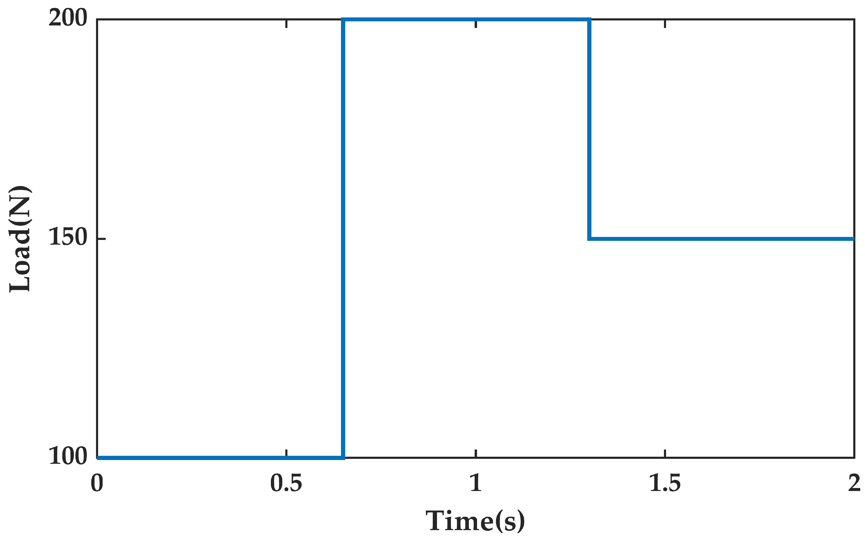
| PI | Start with 100 N load | 3.4286 × 10⁻⁴ | 6.8789 × 10⁻⁴ |
| Sudden 100 N load | 3.1952 × 10⁻⁴ | 6.4449 × 10⁻⁴ | |
| Sudden drop of 50 N load | 4.1426 × 10⁻⁴ | 9.0252 × 10⁻⁴ | |
| MFAC | Start with 100 N load | 1.4326 × 10⁻⁴ | 2.3843 × 10⁻⁴ |
| Sudden 100 N load | 1.0365 × 10⁻⁴ | 1.9340 × 10⁻⁴ | |
| Sudden drop of 50 N load | 1.4080 × 10⁻⁴ | 2.3835 × 10⁻⁴ | |
| MFAPC | Start with 100 N load | 6.9372 × 10⁻⁵ | 1.3078 × 10⁻⁴ |
| Sudden 100 N load | 8.0155 × 10⁻⁵ | 1.9047 × 10⁻⁴ | |
| Sudden drop of 50 N load | 7.0799 × 10⁻⁵ | 1.1364 × 10⁻⁴ | |
| IESO−MFAPC | Start with 100 N load | 1.8293 × 10⁻⁵ | 3.7948 × 10⁻⁵ |
| Sudden 100 N load | 1.7799 × 10⁻⁵ | 3.6790 × 10⁻⁵ | |
| Sudden drop of 50 N load | 1.7812 × 10⁻⁵ | 3.3845 × 10⁻⁵ |
| Controller | Disturbance | Root Mean Square Error | Maximum Error |
|---|---|---|---|
| MFAC | Start with 100 N load | 2.0649 | 5.2132 |
| Sudden 100 N load | 2.0494 | 5.1139 | |
| Sudden drop of 50 N load | 2.0628 | 5.2103 | |
| MFAPC | Start with 100 N load | 2.0609 | 5.1443 |
| Sudden 100 N load | 2.0471 | 5.3514 | |
| Sudden drop of 50 N load | 2.0515 | 5.1293 | |
| IESO−MFAPC | Start with 100 N load | 2.0893 | 5.3546 |
| Sudden 100 N load | 2.0758 | 5.3908 | |
| Sudden drop of 50 N load | 2.0864 | 5.3667 |
Publisher’s Note: MDPI stays neutral with regard to jurisdictional claims in published maps and institutional affiliations. |
© 2022 by the authors. Licensee MDPI, Basel, Switzerland. This article is an open access article distributed under the terms and conditions of the Creative Commons Attribution (CC BY) license (https://creativecommons.org/licenses/by/4.0/).
Share and Cite
Wang, X.; Yao, S.; Qu, C.; Wang, Y.; Xu, Z.; Huang, W.; Wang, H. Direct Thrust Force Control of Primary Permanent Magnet Linear Motor Based on Improved Extended State Observer and Model-Free Adaptive Predictive Control. Actuators 2022, 11, 270. https://doi.org/10.3390/act11100270
Wang X, Yao S, Qu C, Wang Y, Xu Z, Huang W, Wang H. Direct Thrust Force Control of Primary Permanent Magnet Linear Motor Based on Improved Extended State Observer and Model-Free Adaptive Predictive Control. Actuators. 2022; 11(10):270. https://doi.org/10.3390/act11100270
Chicago/Turabian StyleWang, Xiuping, Shunyu Yao, Chunyu Qu, Yiming Wang, Zhangwei Xu, Wenbin Huang, and Hai Wang. 2022. "Direct Thrust Force Control of Primary Permanent Magnet Linear Motor Based on Improved Extended State Observer and Model-Free Adaptive Predictive Control" Actuators 11, no. 10: 270. https://doi.org/10.3390/act11100270
APA StyleWang, X., Yao, S., Qu, C., Wang, Y., Xu, Z., Huang, W., & Wang, H. (2022). Direct Thrust Force Control of Primary Permanent Magnet Linear Motor Based on Improved Extended State Observer and Model-Free Adaptive Predictive Control. Actuators, 11(10), 270. https://doi.org/10.3390/act11100270