Article

A New Method for Identifying Kinetic Parameters of Industrial Robots

1
Academy for Enigineering and Technology, Fudan University, Shanghai 200433, China
2
Guanghua Lingang Engineering Application and Technology R & D (Shanghai) Co., Ltd., Shanghai 201306, China
*
Author to whom correspondence should be addressed.
Actuators 2022, 11(1), 2; https://doi.org/10.3390/act11010002
Submission received: 29 November 2021 / Revised: 20 December 2021 / Accepted: 21 December 2021 / Published: 23 December 2021
(This article belongs to the Special Issue Dynamics and Control of Robot Manipulators)

Abstract

:
Identifying the kinetic parameters of an industrial robot is the basis for designing a controller for it. To solve the problems of the poor accuracy and easy premature convergence of common bionic algorithms for identifying the dynamic parameters of such robots, this study proposed simulated annealing with similar exponential changes based on the beetle swarm optimization (SEDSABSO) algorithm. Expressions for the dynamics of the industrial robot were first obtained through the SymPyBotics toolkit in Python, and the required trajectories of excitation were then designed to identify its dynamic parameters. Following this, the search pattern of the global optimal solution for the beetle swarm optimization algorithm was improved in the context of solving for these parameters. The global convergence of the algorithm was improved by improving the iterative form of the number N of skinks in it by considering random perturbations and the simulated annealing algorithm, whereas its accuracy of convergence was improved through the class exponential change model. The improved beetle swarm optimization algorithm was used to identify the kinetic parameters of the Zhichang Kawasaki RS010N industrial robot. The results of experiments showed that the proposed algorithm was fast and highly accurate in identifying the kinetic parameters of the industrial robot.

1. Introduction

Kinetic parameters are the main factor influencing the control of fast and highly precise movements of industrial robots [1]. The process of identifying of their kinetic parameters is usually divided into a number of steps, such as kinetic modeling, designing the excitation trajectory, data acquisition, and identifying and verifying the kinetic parameters [2]. Gautier et al. used a two degree-of-freedom (DOF) robot as the object of study and applied the extended Kalman filter and the least-squares method to identify its parameters. Memar used the SCHUNK Powerball LWA 4P as an experimental object, constructed a dynamics model for it, and implemented the least-squares method to identify the dynamic parameters of the industrial robot [3]. However, the least-squares method is susceptible to measurement noise that lowers its accuracy [4]. Fu et al. [5] used the particle swarm optimization (PSO) algorithm with least squares to identify the kinetic parameters of a seven-DOF collaborative robot in Xinsong, but PSO can easily fall into the local optimum owing to poor population diversity in the late stage of processing that reduces the accuracy of identification of the parameters. Ding et al. [6] identified the dynamics of the robot by using the genetic algorithm, but the process of coding of the algorithm is cumbersome.
Summarizing the existing research, it is found that the identification of robot dynamics parameters is a high-dimensional function problem. Common algorithms are either the PSO accuracy is not high enough, or the genetic algorithm coding is more complicated, so a simple programming, strong anti-interference ability, and convergence accuracy are needed. High algorithm. BSO is a bionic algorithm recently proposed, which mainly uses the principles of PSO and the Beetle Antenna Search (BAS) algorithm, so it has the advantage of simple programming [7,8,9]. This article proposes SEDSABSO on the basis of BSO.SEDSABSO combined random perturbation-based behavior and the simulated annealing (SA) algorithm with the global optimal solution of the BSO [10,11] to improve its ability to search for global optimal particles as well as the manner of changes in N particles through an exponential decay model. This improved the convergence of BSO without affecting its computational complexity. Therefore, using the SEDSABSO algorithm for robot dynamic parameter identification will have the advantages of simple programming, high convergence accuracy, and fast iteration speed.
The rest of the paper is organized as follows. Section 2 describes the D-H and the dynamic parameters of the RS010N robot and then linearized them through the SymPyBotics toolkit in Python. In Section 3, the genetic algorithm toolbox in MATLAB was used to design the excitation trajectories required to identify the dynamic parameters of the robot. Section 4 describes the principle of the SEDSABSO algorithm and its process for the identification of robot dynamics parameters. In Section 5, the minimum set of parameters for the dynamics of the RS010N robot was identified and was used to compare the per-formance of the SEDSABSO, BSO, and LDWPSO algorithms. The results verified the accuracy and effectiveness of the proposed algorithm [12].

2. Robotic arm Dynamics Model

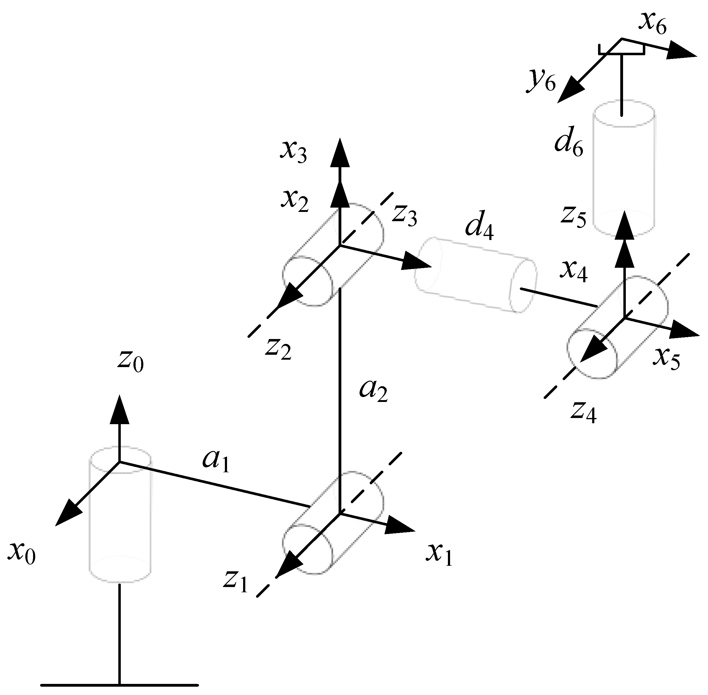
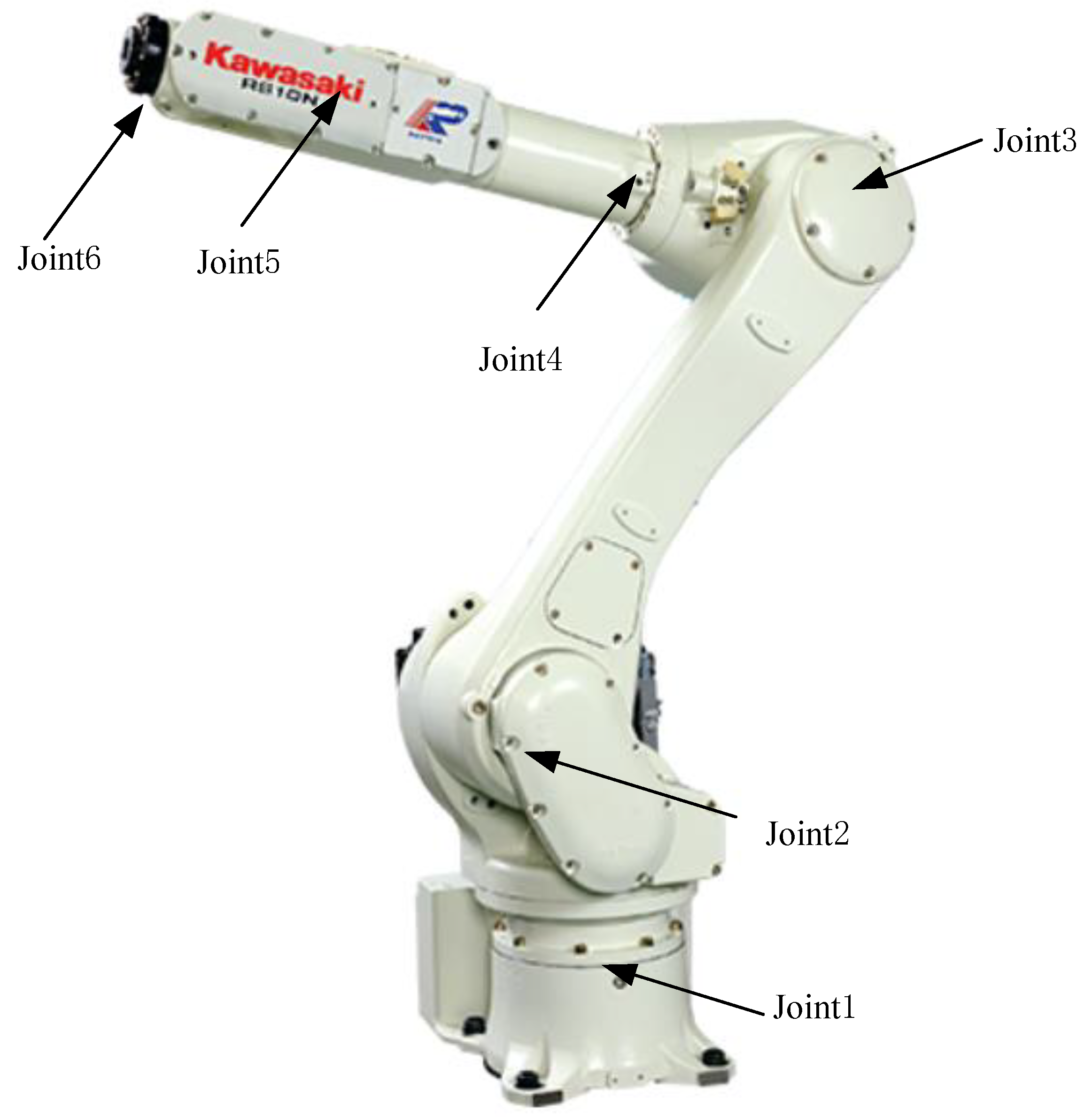
2.1. RS010N Industrial Robots

In this paper, we used the Zhichang Kawasaki RS010N robot as the research object. Figure 1 shows its structural configuration, and Figure 2 shows the configuration of its DH coordinates. The RS010N robot is a typical six-DOF industrial robot. Because the kinetic parameters of its three rear joints are much smaller than those of its three front joints, the former have a smaller influence on the accuracy of control of the robot’s motion. Thus, we considered only the first three joints of the RS010N industrial robot here [13].

2.2. Dynamics Modeling

For an n-link robotic arm, the dynamics as modeled by the Newton-Euler method can be described as
τ = D ( q ) q ¨ + C ( q , q ˙ ) + G ( q )
In Equation (1), τ denotes the driving moment, q denotes the vector of the position of the joints, and q ˙   and q ¨ denote vectors of the velocity and acceleration of the joints, respectively. D(q) denotes the inertial matrix, C(q,   q ˙ ) denotes the Koch and centrifugal force terms, respectively, and G(q) denotes the gravitational force term [14].
According to the improved Newtonian–Eulerian dynamics, the above equation can be transformed into
τ = Φ ( q , q ˙ , q ¨ ) P
where Φ is the observation matrix with a size of n ∗ 12n, and P denotes the vector of the inertial parameters of the robot arm.

2.3. Minimum Set of Parameters for the Dynamical Model

The parameters of the first three joint linkages of the RS010N six-freedom robot are shown in Table 1 below. a0 = 350 mm, a1 = 1035 mm.
The kinetic parameters are shown in Table 2.
We obtained the minimum set of parameters and related expressions for them through the SymPyBotics toolkit in Python.
[ I 1 x x I 1 y y I 1 z z I 1 x y I 1 x z I 1 y z m 1 x 1 y 1 z 1 F 1 c F 1 v I 2 x x I 2 y y I 2 z z I 2 x y I 2 x z I 2 y z m 2 x 2 y 2 z 2 F 2 c F 2 v I 3 x x I 3 y y I 3 z z I 3 x y I 3 x z I 3 y z m 3 x 3 y 3 z 3 F 3 c F 3 v ] Linearization [ I 1 z z + I 2 z z + I 3 z z + 2 * a 1 * I 1 x + m 1 * a 1 2 ( m 2 + m 3 ) * ( a 2 2 a 1 2 ) F 1 c F 1 v I 2 x x I 2 y y ( m 2 + m 3 ) * a 2 2 I 2 x y I 2 x a 2 * ( I 2 z I 3 y ) I 2 y z I 2 z z ( m 2 + m 3 ) * a 2 2 I 2 x + ( m 2 + m 3 ) * a 2 I 2 y F 2 c F 2 v I 3 x x I 3 z z I 3 x y I 3 x z I 3 y y I 3 y z I 3 x I 3 z F 3 c F 3 v ]
According to Equation (3) above, the 36 kinetic parameters of the robot were linearized to 21, and the kinetic model can be written in the following form
τ = Φ b ( q , q ˙ , q ¨ ) p b
where Φb is the full-rank observation matrix and Pb denotes the underlying parameter vector of the robotic arm.

3. Incentive Track Design

The commonly used excitation trajectory when identifying the kinetic parameters of industrial robots is the finite-term Fourier series [15,16]. It can be expressed in the following form:
θ ¨ i ( t ) = n = 1 N a n n w f sin ( n w f t ) b n n w f cos ( n w f t )
θ ˙ i ( t ) = n = 1 N a n cos ( n w f t ) b n sin ( n w f t )
θ i ( t ) = θ 0 + n = 1 N a n n w f sin ( n w f t ) b n n w f cos ( n w f t )
wf denotes the fundamental frequency of the Fourier series. Each Fourier series contains an, bn, and θ0. N represents the number of harmonic terms of the Fourier series. Because each Fourier series has 2N + 1 parameters, n represents the number of 1 … 2N + 1.
The constraints on the RS010N robot are shown in Table 3.
When the robot moved, the observation matrix w was obtained by recording the angle, velocity, and acceleration of the joints of the robot in Φb. n denotes the nth sample.
w = [ Φ b ( q 1 , q ˙ 1 , q ¨ 1 ) Φ b ( q n , q ˙ n , q ¨ n ) ]
Adaptation function of the incentive trajectory.
y = C o n d ( w ) + P
where P denotes a penalty function and Cond denotes the number of conditions of the acquisition matrix. When the trajectory of the industrial robot satisfies the above constraint, P = 0, and P = 108 otherwise. The excitation of the first three joints of the RS010N was obtained by the genetic algorithm toolbox in MATLAB as shown in Figure 3.

4. SEDSABSO for the Identification of Industrial Robot Dynamics Parameters

4.1. Improving Global Optimal Search

Owing to the large number of dynamic parameters of the industrial robot that needed to be identified, their solution was a high-dimensional function optimization problem with certain constraints. The BSO used to obtain the kinetic parameter identification of industrial robots easily falls into the premature phenomenon, so the global optimal solution search mode of BSO and the iterative change form of the number N of tennies in the iterative process of BSO are improved in this paper.

BSO

BSO was proposed by Wang et al. based on the PSO and the Aspen whisker algorithm. The position of a body in BSO represents a feasible solution to the optimization problem. The formula to update BSO is:
x i j ( t + 1 ) = x i j ( t ) + λ v i j ( t + 1 ) + ( 1 λ ) ξ i j ( t )
where t denotes the number of iterations of the skink, i denotes the number of skinks in the skink population, j denotes the dimensionality of the problem to be solved, λ denotes xij(t + 1) denotes the position of skink i in the skink population at t + 1 iterations, ξij(t) denotes the position of the ith skink moving autonomously, and vij(t + 1) denotes the velocity of the ith skink. It is expressed as:
v i j ( t + 1 ) = w v i j ( t ) + c 1 r 1 ( p i j ( t ) x i j ( t ) ) + c 2 r 2 ( g i j ( t ) x i j ( t ) )
w denotes inertial weight, pij(t) denotes the optimal position of individual i after t iterations of the Aspen population, xij(t) denotes the given position of i after t iterations, gij(t) denotes the optimal position of the Aspen population after t iterations, c1 and c2 denote adjustment factors, and r1 and r2 denote random numbers within the interval [0,1]
ξ i j ( t + 1 ) = δ ( t ) * V i j ( t ) * s i g n ( f ( x l j ( t ) ) f ( x r j ( t ) ) )
In Equation (12), sign(.) denotes the sign function, ξij(t + 1) denotes the t + 1th motion position searched by Aspen autonomously, δ(t) denotes the step size of the Aspen individual after t iterations, and f(xlj(t)) and f(xrj(t)) denote the fitness values of the left and right whiskers of the Aspen, respectively.
The positions of the left and right whiskers of the Aspen are indicated by:
x l j ( t + 1 ) = x l j ( t ) + V i j ( t ) d 0 / 2 x r j ( t + 1 ) = x r j ( t ) V i j ( t ) d 0 / 2
xlj(t + 1) denotes the position of the left whisker in iteration t + 1, xrj(t + 1) is the t + 1 right whisker position, and d0 denotes the distance between the whiskers.

4.2. Improving BSO

4.2.1. Improved Global Optimal Solution

The global optimal particle Pg of BSO is randomly perturbed. Then, the new solution after perturbation is selected by the metropolis criterion of SA to improve the global convergence of BSO.
(1)
Simulated annealing algorithm
The simulated annealing algorithm controls the probability of jumping out of the local optimum by setting the temperature. The algorithm evaluates whether to jump out of the worse solution by the metropolis criterion. The procedure is as follows:
  • The algorithm is initialized, and an initial solution x is randomly generated as the optimal solution.
  • A new solution xt is obtained in the vicinity of the initial solution, denoted by ∆f = f(xt) − f(x).
  • The new solution xt is accepted according to min{1,exp(−∆f/Tk)}>random. Tk denotes the temperature and exp denotes the exponential function, with natural number e as the base.
(2)
Random behavior
Stochastic behavior is a search behavior that can improve the diversity of algorithmic populations and is widely used in a variety of intelligent algorithms, such as in the foraging behavior within the fish swarm algorithm to search for food and the wandering behavior of the wolf pack algorithm to sense the scent of prey in the air in a random pattern [17,18]. Inspired by this, we incorporated stochastic behavior into BSO, and the optimal particles in it were randomly perturbed during each iteration to enhance its ability to escape from the local optimal solution to improve global convergence:
Pgnew = Pg ∗ (1 + rand)
where Pgnew denotes the new solution after the random perturbation of the optimal particle of the Aspen swarm, and rand represents a random number from zero to one. The fitness value of the optimal particle pg of BSO was compared with that of the global optimal particle Pgnew for random perturbation; then, the new solution was accepted according to the metropolis criterion of SA. BSO performed q random perturbations of its global optimal solution in each iteration.

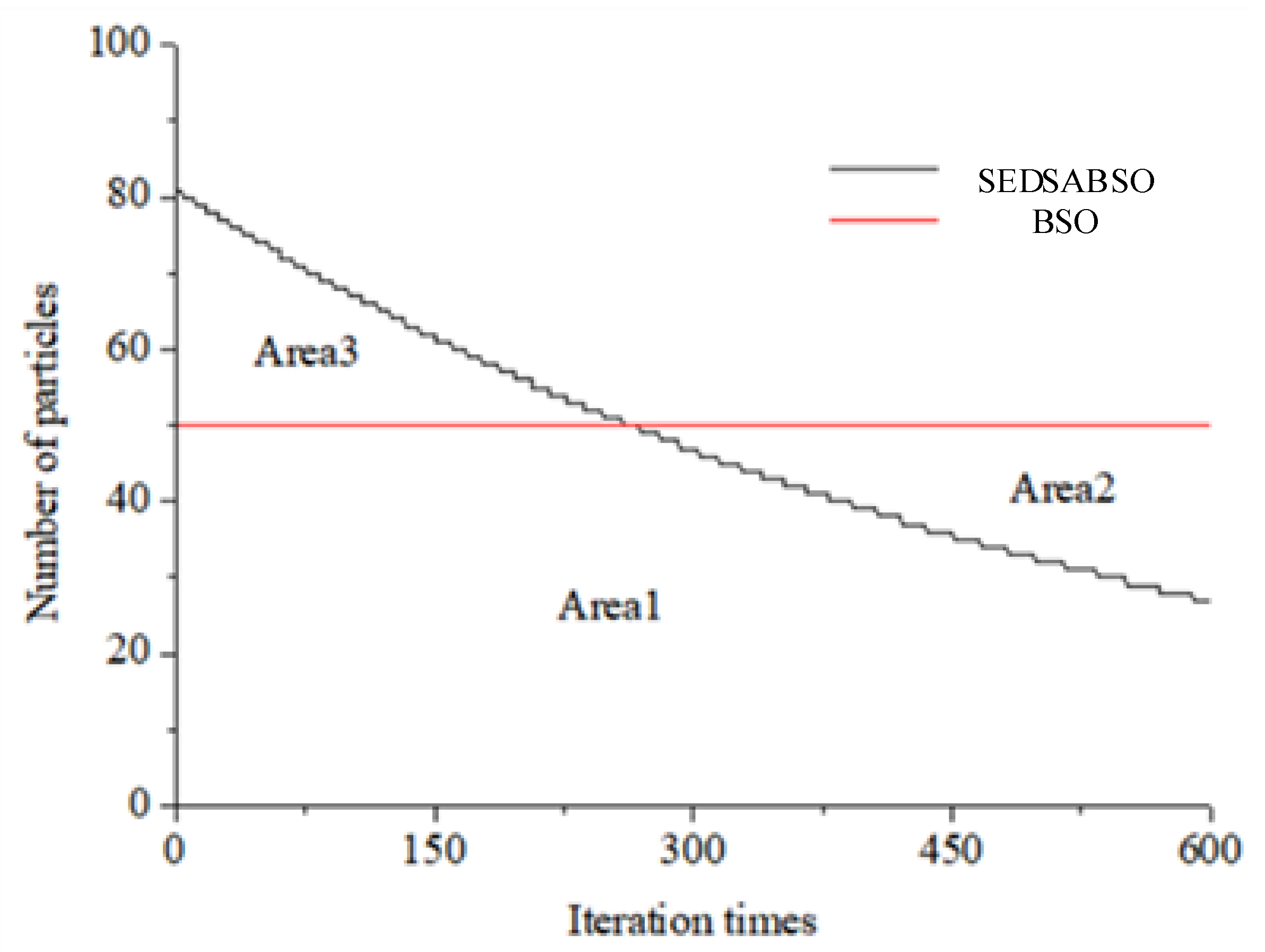
4.2.2. Improved Iterative Approach to N Particles of the Aspen Swarm

Each skyline of BSO represents a potential solution to the problem. Assuming that the number of skylines in each iteration of BSO is N, the maximum number of its iterations is Maxdt, and the duration of the iteration of a single skyline is t, the total complexity of iterations of BSO is N*Maxdt*t [19]. In solving a high-dimensional function problem, similar to determining the dynamic parameters of the industrial robot, the number of particles N at the moment of each iteration of BSO is constant. BSO is based on PSO, and a larger number of particles in PSO yields a higher accuracy of the convergence, but the time needed for convergence also increases.
For example, in previous work, we proposed a two-stage dynamic PSO that changed the number of particles in the swarm by linearly reducing the number of iterations. The experimental results showed that the accuracy of convergence of the algorithm was similar to that of the classical PSO algorithm, which also reflects a side-effect of the latter. The algorithm proposed here also had this property of a high initial accuracy of convergence [20]. Inspired by this, the number N of skinks in the skink swarm was changed dynamically. The number was larger in the early stage of the skink swarm algorithm and smaller in the later stage, such that the total number of skinks did not differ by much and the gap in the durations of their iterations was not large. We fully exploited the high efficiency of the early iterations of the skink swarm algorithm for the accuracy of its solution. The exponentially decreasing rate of curtailment was used for the number of cows N of the Aspen swarm algorithm by drawing on the idea proposed by Wang et al. [21]. That is, the particle swarm algorithm used a larger number of particles to search in the initial stage. With the increase of the number of iterations, the exponentially decreasing number of particle was used to reduce the Aspen number, so as to improve the search efficiency, and the improved iterative formula for the Aspen number is as follows:
N = r o u n d ( e α * N s t a r t )
α = t I n f m a x I n f m i n M a x d t I n f m a x
where Nstart denotes the initial number of skinks of the improved skink herd, i denotes the number of iterations of the skink herd algorithm, Maxdt denotes the maximum number of iterations, and fmax and fmin are the respective maximum and minimum values of the search factor set used to control the number of skinks N.

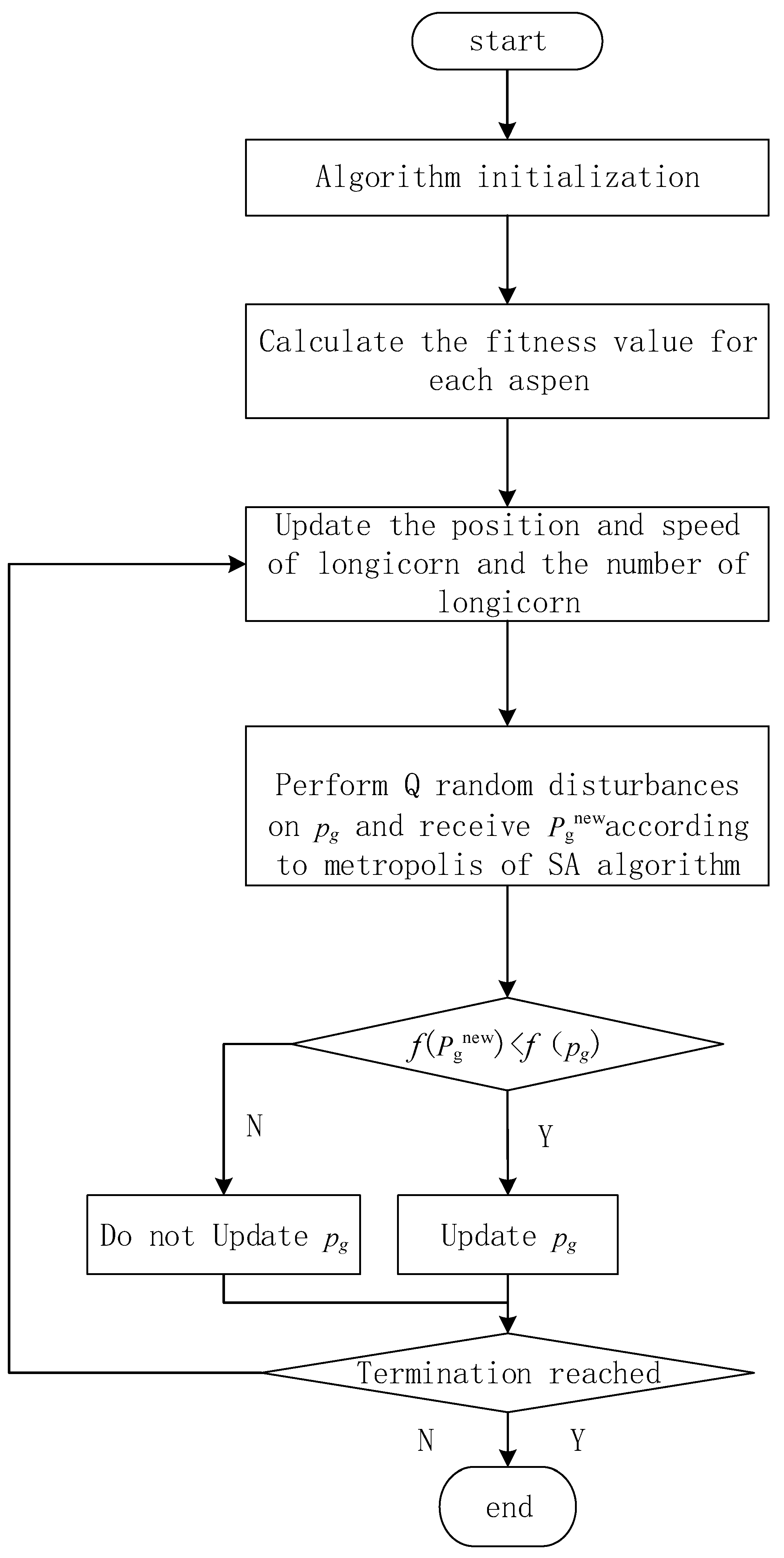
4.3. Robot Dynamic Parameter Identification Based on SEDSABSO

The SEDSABSO process is illustrated below:
From Figure 4, the flow of SEDSABSO for industrial robot dynamics parameter identification is:
(1)
Initialization of the algorithm.
(2)
Obtain SEDSABSO individual and group best-fit values.
(3)
Update the position, velocity, and number of skinks N
(4)
Perform a random perturbation search for the global optimal solution and then accept the searched solution with SA’s Metropolis criterion and cycle through q searches.
(5)
Compare with the global optimal solution obtained in step 3 after passing q times of search and proceed to the next step of the search by merit.
(6)
Determine whether the algorithm ends, and if the termination condition is not satisfied, return to step 3. If it is satisfied, the global optimal solution is output. In turn, the parameters related to industrial robot dynamics are obtained.

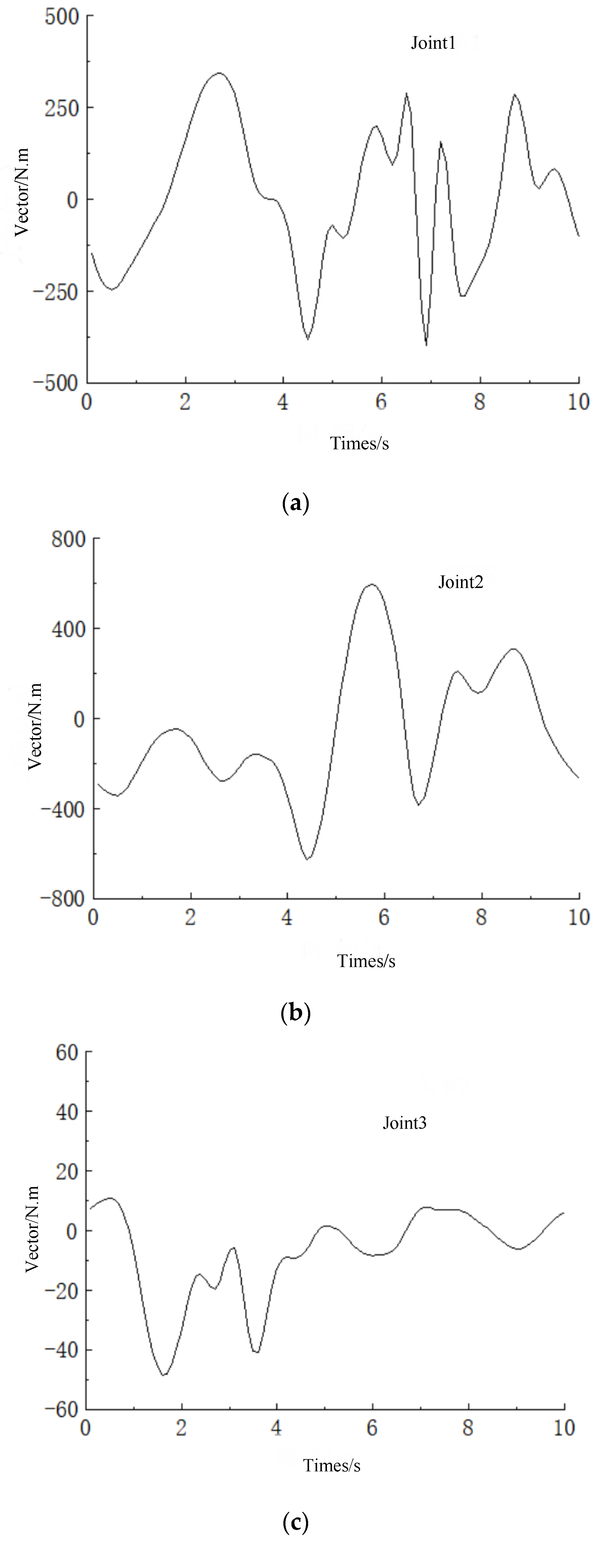
5. Simulation Experiments and Results Analysis

5.1. Adaptation Function

The sum of the absolute values of the difference between the torque of joint recognition and the theoretical torque of the RS010N robot when sampled i times was used as the objective function, as in Equation (17)
i = 1 N a b s ( f k 1 ( i ) f 1 ( i ) ) + a b s ( f k 2 ( i ) f 2 ( i ) ) + a b s ( f k 3 ( i ) f 3 ( i ) )
i = 1, 2, …, N denotes the ith sample of the robot, fk1(i), fk2(i), and fk3(i) denote values of the first, second, and third moments of the joints values for the i robot recognition f1(i), f2(i), f3(i) denotes the theoretical value of the three joint moments sampled by the robot.

5.2. Analysis of Experimental Results

Experimental Parameter Setting

To improve the accuracy of identification of the kinetic parameters, the individual algorithms were initialized uniformly by using a small interval [22]. Then, the dynamic parameters of the robot were solved for by using the SEDSABSO algorithm, BSO algorithm, and linearly decreasing particle swarm algorithm (LDWPSO), where the number of particles N was set to 50 for the BSO and LDWPSO algorithms. The initial population Nstart for SEDSABSO was set to 90, the learning factor was c1 = c2 = 2.0, and the inertial weight w was 0.8. The maximum number of iterations was set to 600. The initial temperature T for simulated annealing was set to 10,000, the decay scale of the annealing coefficient was set to 0.93, the step δ(t) was set to a constant value of 0.05, the adjustment factor λ was 0.9, and the ratio of the Aspen step to the distance between the whiskers, c, was set to two. After many trials, the optimal number of particle perturbations for the population was set to q = 3, fmax was 0.9, and fmin was 0.3. The iteration curves of the Aspen number for SEDSABSO and BSO are shown below:
Figure 5 shows that the number of particles N was constant during iterations of the BSO algorithm. Assuming that the maximum number of iterations was Maxdt and the duration of iteration of each particle was t, the total duration of iterations of BSO was NMaxdt∗t, and NMaxdt is equal to Area1+Area2 in the figure. For the SEDSABSO algorithm, the total iteration time was approximately the product of Figure 5. For the SEDSABSO algorithm, the total iteration time was approximately the product of the area of the class trapezoid enclosed by the dash and the horizontal axis and the time t, i.e., (Area3 + Area1) ∗ t, and since the area of Area3 was not much different from that of Area2, the computational complexity of the improved Amanita group algorithm was approximately the same as that of the standard Amanita group algorithm.
Figure 6 below shows the adaptation iteration curves of each algorithm on an Intel(R) Core(TM) i7-8550U main frequency 4.00 GHz computer with 600 iterations through Matlab 9.1:
From Figure 6, we can see that the SEDSABSO algorithm proposed in this paper converges faster and has smaller fitness values than the BSO and LDWPSO algorithms. It is clear that the SEDSABSO algorithm proposed in this paper performs best.
In order to further verify the advanced level of the SEDSABSO algorithm, this paper ran each of the above three algorithms ten times and found the average fitness and average time as follows in Table 4:
From Table 4, we can see that the average fitness values of the three algorithms after ten runs were only 0.95 for SEDSABSO, 1.12 for BSO, and 1.18 for LDWPSO, further confirming the stability and effectiveness of the proposed SEDSABSO algorithm. It can be seen that the average time of SEDSABSO was better than that of BSO, further proving the analysis in Figure 5. The difference with LDWPSO was not significant, and combined with the average fitness value, it can be seen that SEDSABSO performed optimally.
The linearized kinetic parameters of the RS010N industrial robot had a total of 21 minimum parameter sets, and the results of the kinetic parameters identified by SEDSABSO, BSO, and LDWPSO are shown in Table 5 below; the absolute errors between the identified kinetic parameters and the actual parameters were also obtained.
Taking the second parameter F1c of the set of minimum parameters of the industrial robot in Table 5 as an example, the absolute errors identified by BSO and LDWPSO were −0.35 and 0.2, respectively, while the absolute error of SEDSABSO was −0.01. On the whole, the SEDSABSO algorithm yielded the smallest error in identifying the kinetic parameters of the industrial robot, while BSO and LDWPSO The kinetic parameters identified by the SEDSABSO algorithm deviated from the theoretical kinetic parameter values, which further reflects the superiority of the SEDSABSO algorithm. The maximum absolute error in the kinetic parameters as identified by the SEDSABSO algorithm was −0.39. The overall error in identification was thus small. The SEDSABSO algorithm can thus identify the kinetic parameters of the robot.

6. Conclusions

(1)
In this paper, a new improved Beetle Antennae Search-QEDSABSO is proposed, which makes a class exponential change to the number of skinks in the iterative process of Beetle Antennae Search and effectively improved the utilization rate of Beetle Antennae Search skinks while the total number of skinks was basically unchanged. Simulation experiments showed that the proposed algorithm is more accurate and faster than the common particle swarm and Beetle Antennae Search in identifying the dynamics parameters of robots. The simulations showed that the proposed algorithm can identify the dynamical parameters of the robot with higher accuracy and faster speed than the common particle swarm and Beetle Antennae Search.
(2)
The difficulty in identifying the kinetic parameters of industrial robots lies in the sheer number of variables that need to be determined and the selection of reasonable excitation trajectories. This paper designed the relevant excitation trajectories by using the genetic algorithm and linearized the kinetic parameters of the industrial robot to improve the accuracy of their recognition.
(3)
The work provided the foundation for experiments compensating for the kinetic moments of the industrial robot. The minimum set of parameters of the kinetics could first be obtained by SymPyBotics. Then, the excitation trajectory of the industrial robot was designed by using the genetic algorithm, the data on its kinetic moments were collected, and the moments were identified by the SEDSABSO algorithm. Following this, the theoretical kinetic moments of the robot were calculated and compared with empirically sampled moments to obtain the error. Finally, this error was used to compensate for the kinetic moment of the robot.

Author Contributions

Methodology, B.K.; Software, B.K.; Validation, B.K.; Writing—original draft, B.K.; Writing—review & editing, B.K., S.G. article chart editor, B.K. and D.R. All authors have read and agreed to the published version of the manuscript.

Funding

This research was supported by the national key R & D plan project (2017YFB1301000).

Data Availability Statement

The data used in this study were self-tested and self-collected during the test. As the control method in this paper is still being further optimized, the data cannot be shared at present. Therefore, data sharing is not applicable to this article.

Conflicts of Interest

The authors declare no conflict of interest.

References

  1. Liu, Z.; Zhao, B.; Zhu, H. Sorting Experimental Platform Research on Six-DOF Manipulator. Mach. Des.Manuf. 2013, 27, 210–213. [Google Scholar]
  2. Wu, J.; Wang, J.; You, Z. An overview of dynamic parameter identification of robots. Robot. Comput. Integr. Manuf. 2010, 26, 414–419. [Google Scholar] [CrossRef]
  3. Gautier, M.; Janot, A.; Vandanjon, P.O. A new closed-loop output error method for parameter identification of robot dynamics. IEEE Trans. Control Syst. Technol. 2013, 21, 428–444. [Google Scholar] [CrossRef] [Green Version]
  4. Memar, A.H.; Esfahani, E.T. Modeling and Dynamic Parameter Identification of the SCHUNK Powerball Robotic Arm. In Proceedings of the ASME 2015 International Design Engineering Technical Conferences and Computers and Information in Engineering Conference, Boston, MA, USA, 2–5 August 2015; American Society of Mechanical Engineers: New York, NY, USA, 2015; p. VOSCT08A024. [Google Scholar]
  5. Fu, X.; Yuan, J.; Wang, S.; Wang, N.; Zhang, W. Nonlinear Dynamic Identification of Robotic Manipulators Based on Particle Swarm Optimization Method. Mech.-Electr. Integr. 2017, 023, 3–8. [Google Scholar]
  6. Ding, L.; Wu, H.; Yao, Y.; Li, Y.; Xie, B.H.; Chen, B. Parameters Identification of Industrial Robots Based on WLS-ABC Algorithm. J. South China Unive. Technol. (Natl. Sci. Ed.) 2016, 44, 90–95. [Google Scholar]
  7. Jiang, X.; Li, S. BAS: Beetle antennae search algorithm for optimization problems. arXiv 2017, arXiv:1710.10724. [Google Scholar] [CrossRef]
  8. Chen, T.; Yin, H.; Jiang, H. Particle Swarm Optimization Algorithm Based on Beetle Antennae Search for Solving Portfolio Problem. Comput. Syst. Appl. 2019, 28, 171–176. [Google Scholar]
  9. Wang, T.; Long, Y.; Qiang, L. Beetle Swarm Optimization Algorithm: Theory and Application. arXiv 2018, arXiv:1808.00206. [Google Scholar] [CrossRef]
  10. Zhou, T.; Qian, Q.; Fu, Y. Fusion Simulated Annealing and Adaptive Beetle Antennae Search Algorithm. Commun. Technol. 2019, 52, 1626–1631. [Google Scholar]
  11. Khan, A.H.; Cao, X.; Li, S.; Katsikis, V.N.; Liao, L. BAS-ADAM:an ADAM based approach to improve the performance of beetle antennae search optimizer. IEEE/CAA J. Autom. Sin. 2020, 7, 461–471. [Google Scholar] [CrossRef]
  12. Xu, C. Research on Dynamic Parameter Identification And Feedforward Control of Articulated Robots; Southeast University: Nanjing, China, 2017. [Google Scholar]
  13. Zhang, J.; Duan, J. Robot Dynamic Parameter Identification Based on Improved Differential Evolution Algorithm. J. Beijing Union Univ. 2020, 1, 49–55. [Google Scholar]
  14. Craig, J.J. Introduction to Robotics Mechanics and Control; Pearson Prentice Hall: Upper Saddle River, NJ, USA, 2005. [Google Scholar]
  15. Sun, Y.; Zhou, B.; Meng, Z. Dynamic Parameter Identification of Industrial Robot Based on Genetic Algorithm. Ind. Control Comput. 2017, 9, 4–6. [Google Scholar]
  16. Swevers, J.; Ganseman, C.; De Schutter, J.; Van Brussel, H. Experimental robot identification using optimised periodic trajectories. Mech. Syst. Signal Process. 1996, 10, 561–577. [Google Scholar] [CrossRef]
  17. Jiang, M.; Yuan, D. Wavelet Threshold Optimization with Artificial Fish Swarm Algorithm. In Proceedings of the 2005 International Conference on Neural Networks, Beijing, China, 13–15 October 2005; IEEE Press: Piscataway, NJ, USA, 2005; pp. 569–572. [Google Scholar]
  18. Liu, C.; Yan, X.; Liu, C.; Wu, H. The wolf colony algorithm and applications. Chin. J. Electron. 2011, 20, 212–216. [Google Scholar]
  19. Wang, Q.; Li, L.; Lu, C.; Sun, F. Average Computational Time Complexity Optimized Dynamic Particle Swarm Optimization Algorithm. Comput. Sci. 2010, 37, 191. [Google Scholar]
  20. Kou, B.; Guo, S.; Ren, D. Geometric parameter calibration of industrial robot based on improved particle swarm optimization. J. Harbin Inst. Technol. 2021, 49, 61–64. [Google Scholar]
  21. Wang, Y.G.; Qu, T.T.; Li, S. Disruption particle swarm optimization algorithm based on exponential decay weight. Appl. Res. Comput. 2020, 37, 1020–1024. [Google Scholar]
  22. Liu, Y.; Li, G.X.; Xia, D.; Xu, W.F. Identifying Dynamic parameters of a space robot based on improved genetic algorithm. J. Harbin Inst. Technol. 2010, 42, 1734–1739. [Google Scholar]
Figure 1. RS010N robot.
Actuators 11 00002 g001
Figure 2. RS010N Robot DH coordinate system.
Actuators 11 00002 g002
Figure 3. The excitation trajectory of the first three joints of the RS010N robot. (a) First joint motivation. (b) Second joint motivation. (c) Third joint motivation.
Actuators 11 00002 g003
Figure 4. SEDSABSO algorithm flow chart.
Actuators 11 00002 g004
Figure 5. SEDSABSO and BSO Variation curve of number N of longicorn beetles.
Actuators 11 00002 g005
Figure 6. Iterative curve of the algorithm.
Actuators 11 00002 g006
Table 1. RS010N connecting rod parameters.
iαi−1/radai−1/mmdi/mmθi/rad
1pi/2a00θ1
2−pi/2a10θ2
3000θ3
Table 2. Actual kinetic parameters.
Member Number123
Ixx/(kg·m2)36.33−10.027.74
Iyy/(kg·m2)40.617.051.02
Izz/(kg·m2)36.3311.619.81
Ixy/(kg·m2)0.006.143.34
Ixz/(kg·m2)0.005.93−3.42
Iyz/(kg·m2)0.00−7.82−0.29
m/(kg)18.3325.1820.47
x/(mm)0.00122.41152.34
y/(mm)110.11163.8190.24
z/(mm)0.0073.36−34.21
Fc (N·m)0.000.000.00
Fv (N·m)0.000.000.00
Table 3. RS010N robot joint constraints.
ParameterJoint iMinMax
1−180180
Angle2−60140
3−18080
1−125125
Angle velocity2−100100
3−165165
1−4545
Angle acceleration2−4040
3−7575
Table 4. Comparison of average fitness values.
AlgorithmAverage FitnessAverage Time/s
SDESABSO0.9516.93
BSO1.1217.31
LDWPSO1.1812.73
Table 5. Identification of dynamic parameters.
Dynamic Minimum ParametersTheoretica
Value
SEDSABSO
Identification Value
BSO
Identification Value
LDWPSO
Identification Value
SEDSABSO
Absolute Error
BSO
Absolute Error
LDWPSO
Absolute Error
I1yy + I2yy + I3zz + 2 ∗ a1I1x + m1a12 − (m2 + m3) ∗ a2216.4116.8016.8916.82−0.39−0.48−0.41
F1c00.010.35−0.20−0.01−0.350.2
F1v0−0.07−0.210.220.070.21−0.22
I2xxI2yy + (m2 + m3) ∗ a2231.8331.7731.9232.210.06−0.09−0.38
I2xy6.145.785.126.120.361.020.02
I2xa2 ∗ (I2zI3y)5.765.546.225.830.22−0.46−0.07
I2yz−7.82−7.84−7.72−8.100.02−0.10.28
I2zz − (m2 + m3) ∗ a22−37.29−37.11−37.30−37.94−0.180.010.65
I2x + (m2 + m3) ∗ a2247.3747.2947.5247.270.08−0.150.1
I2y0.160.130.090.270.030.07−0.11
F2c00.14−0.02−0.08−0.140.020.08
F2v0−0.21−0.23−0.030.210.230.03
I3xxI3zz−2.07−2.20−2.40−1.510.130.33−0.56
I3xy3.343.243.254.570.100.09−1.23
I3xz−3.42−3.34−2.95−4.10−0.08−0.470.68
I3yy1.020.771.12−0.850.25−0.11.87
I3yz−0.290.10−0.34−1.42−0.390.051.13
I3x0.150.110.12−0.040.040.030.19
I3z−0.0340.00−0.160.04−0.0340.126−0.074
F3c00.18−0.13−1.20−0.180.131.2
F3v00.06−0.34−0.1−0.060.340.1
Publisher’s Note: MDPI stays neutral with regard to jurisdictional claims in published maps and institutional affiliations.

