A Novel Design and Performance Evaluation Technique for a Spool-Actuated Pressure-Reducing Valve

Abstract

Solenoid-actuated pressure-reducing valves are commonly used in hydraulic machinery. Most studies on solenoid-actuated pressure control devices are focused on the electrical input signals or on the control techniques for the solenoid valves, but no study has been done that determines the influence of the design parameters on the valve’s output. Before designing a controller, it is imperative to know the valve’s performance by determining the significance of each valve parameter. In this study, established physical laws from fluid dynamics and mechanics are used to build a model that is solved using the ODE 45 solver of Simulink in the time domain. The actuating force, up to 15 N, exerted on the spool and the inlet pressure, ranging from 50 to 80 bar, are obtained through experimentation. It is found that the output pressure fluctuates significantly if the outlet is blocked, while at the fully opened outlet condition, a flow rate of 12 (L/min) was obtained. A pin diameter of 2.15 mm enables us to vary the output pressure between 0 and 41 bar. We found that higher inlet pressure leads to lower output pressure as the outlet is opened. No linearization of the actual mathematical model is performed, which makes the study unique.

1. Introduction

Power transmission that involves compact machinery and extreme forces is only possible with the use of hydraulic equipment. With sufficient means of controlling the pressure and flow in a hydraulic system, the movement of mechanical loads can be controlled. As is clear from the studies done in the past, the two most important variables to be controlled in a hydraulic control system are flow rate and pressure [1,2,3,4]. That is why solenoid-actuated pressure control valves are widely used in modern hydraulic machinery to perform functions, such as motion control of multi-actuator systems [5]. Pressure relief valves are used for safety or pressure limiting functions, while pressure-reducing valves are used to draw one or multiple low-pressure outputs from a higher pressure source. In any case, a poppet or a spool is used to actuate the valve with the help of a solenoid actuator or some other force exerting means.

Pressure control valves in pneumatic applications are commonly referred to as pressure regulators; however, in hydraulic applications, they are usually called pressure-reducing valves. Such devices are applied to numerous pneumatic and hydraulic applications and use different types of actuators for their functioning. Solenoid-actuated pressure-reducing valves are used in swashplate control mechanisms of variable displacement pumps [6,7], in process industries, hydrogen dispensing from high pressure [8], aircraft and aerospace industry [9], oxy-fuel welding and cutting, inlet flow to a pressure reactor, in domestic water distribution networks and in mining industries [10]. The spool-actuator used in this study has a unique geometry and can be used in the swash plate control of variable displacement pumps to build a pressure compensated flow control mechanism.

Pressure-reducing valves have been studied by many researchers in the recent past. Most of these studies involve the use of physical laws to model the valve and its actuating mechanism. In [11], a pressure-reducing valve used in automotive applications was studied where two different mathematical models were formulated. One was called the input-output mathematical model, and the other a state-space model. However, both the models involved linear approximations of the original equations. In this study, linearization is avoided, and the original model is used. Furthermore, in [11], while solving the model through simulation, the flow rate was considered constant and controllable and was not treated as an output variable as is considered in this study. A study on the pressure-reducing valve by [12] made use of commercial software, AMESIM, for the simulation of the valve that focused primarily on how the throttling flow area affects the valve’s performance, i.e., round flow area was compared with waist shaped flow area.

Some studies treat the pressure-reducing valve as a small component of a larger system, whereby the focus is on the overall system and not on the reducing valve actuator [13,14,15,16]. In these studies, the valve intricacies, such as the spool or actuating element’s size or mass, flow opening area gradient etc., are not discussed. In [13], a static gain compensator was used in front of the PID controller to stabilize the instabilities arising due to high gain at low flow rates, but the compensator was designed through a linear time-invariant model for the valve while treating it as a small part of the piping network. Similarly, the study done by [16] experimentally investigates the behavior of a pressure-reducing valve’s transients installed along a pipe. On the other hand, in this study, we put the pressure-reducing valve and its spool actuator under the microscope to see how it responds if different factors, including the flow rate, are changed. We do not focus on the piping that may be connected to the valve, but that can be done once the valve behavior is understood and investigated. Through this study, we were able to verify that a small outlet flow rate affects the fluctuations in pressure in a way that is in line with the deductions made by [13,14]. This research enables us to accurately predict the trend of such oscillations with the change in flow rate. We examine this phenomenon by changing the orifice area at the valve’s outlet.

Flow force is an important aspect of a valve. Extensive work on flow forces in spool valves has been done in the past [17,18]. These studies are based on the desire to reduce the negative effect of flow forces or to compensate them using different techniques. To have an accurate valve model, the flow forces need to be properly known at different stages of valve actuation. The flow force on the spool depends on the flow dynamics resulting from the spool movement as well as the locations of inlet or outlet ports, as taken into account in this study. Flow forces are classified into steady-state and transient flow forces. In this work, flow forces are modeled through well-documented governing and empirical equations while using the geometrical features of the actuating spool. Furthermore, the implications of flow forces are determined for the higher opening of the valve’s outlet orifice.

Spool-actuated pressure-reducing valves can be used in the independent metering valves developed for modern excavators [19]. The meter-in edges and meter-out edges of independent metering excavator cylinders are separately controlled, which is why they are called independent metering systems. They employ flow control valves, which may use solenoid-actuated pressure-reducing valves to actuate the flow control spool of the main flow control valve in order to control the flow going into or out of the cylinder [20].

To develop a pressure-reducing valve or optimize its performance for a certain application, the valve’s actuating element (e.g., spool or poppet) needs to be carefully designed and analyzed. Very few studies discuss the fine details involved in the governing equations of the system’s fluid and spool kinetics. The spool used in this study is actuated by a solenoid to control the valve’s outlet pressure. The estimation and analysis of the solenoid-actuated pressure-reducing valve’s performance for varying design parameters of the valve is performed. That is why this work may serve as guidance for those who want to design a pressure-reducing valve for a certain output pressure with an available hydraulic power unit and a solenoid actuator.

Pressure control can be achieved by two methods, i.e., by limiting the flow entering a control volume or by limiting the flow exiting the control volume. Pressure-reducing valves, unlike pressure relief valves, control pressure in a chamber by sensing the pressure at the valve outlet and limiting the flow entering through the inlet based on the sensed outlet pressure. Therefore, the maximum steady-state pressure that can be achieved at the outlet is always less than or equal to the pressure at the valve’s inlet.

In this study, we start with the structural/geometrical description and working mechanism of the valve, followed by the detailed mathematical modeling through the use of physical laws, i.e., continuity equations, force balance equations and compressibility formula. The assumptions are mentioned and justified, after which the solver ODE-45 (Simulink) is used to run the simulation of the mathematical model. For simulation, the solenoid force is restricted to a value less than 17 N as it corresponds to the experimental test results of a solenoid actuator. The inlet pressure settings are obtained through experiments as well and were used in the simulation as one of the variables. Furthermore, the influence of pin diameter, outlet orifice, inlet pressure, solenoid force and damping orifice on the pressure output and flow rate along with the response time are derived, presented and explained to gain an insight into the performance of the valve and predict its behavior.

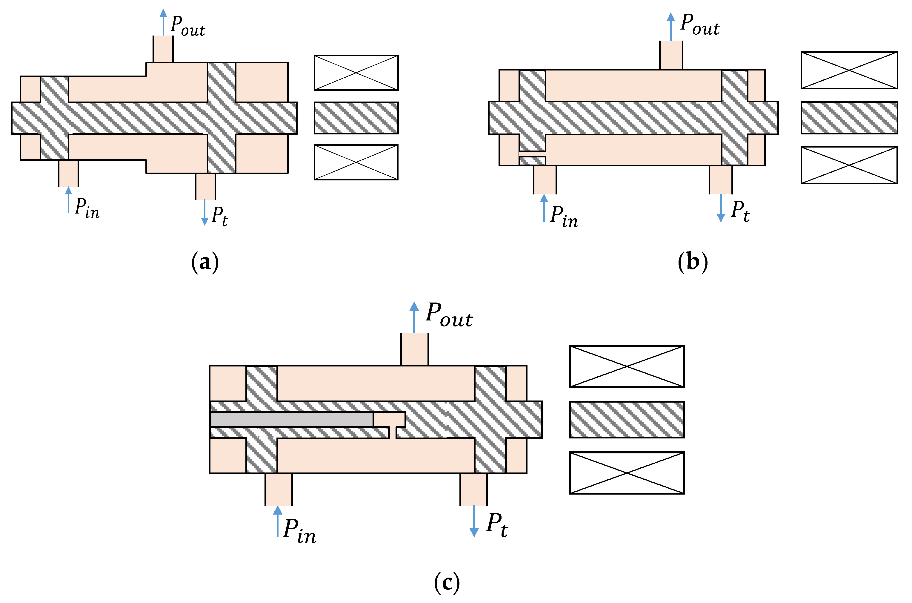
2. Types of Pressure-Reducing Valves Based on Spool Geometry

Based on the spool geometry, pressure-reducing valves can be divided into differential-area and differential-pressure type reducing valves. The difference between these types can be seen in Figure 1.

Once the pressure at the valve outlet develops, the spool is subjected to an unbalanced pressure force. In Figure 1a such an unbalanced force is created by the pressure acting on two different-sized spool lands, while in Figure 1b, the passage through one of the spools helps the spool actuate the valve position.

3. Mathematical Modeling

Governing equations describing the movement of the spool, as well as the flow and pressure variations in the valve chambers and at the valve outlet, are formulated. Relevant assumptions are presented in Section 3.3. The system of equations that constitute the mathematical model of the valve are solved in the time domain without any linearization or conversion to the time domain. The mathematical model enables us to examine the influence of design parameters and actuating solenoid force on the resulting pressure-flow characteristics.

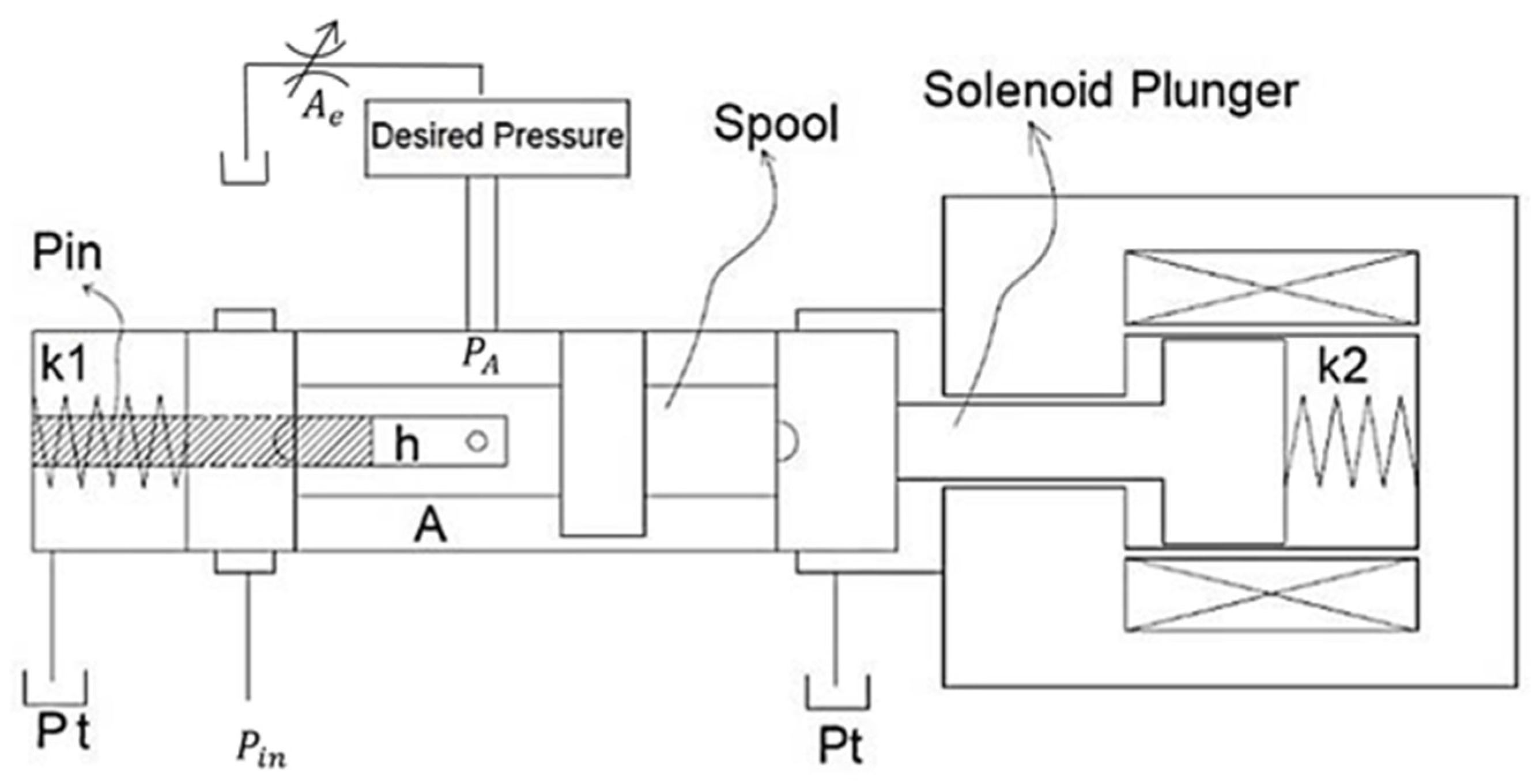
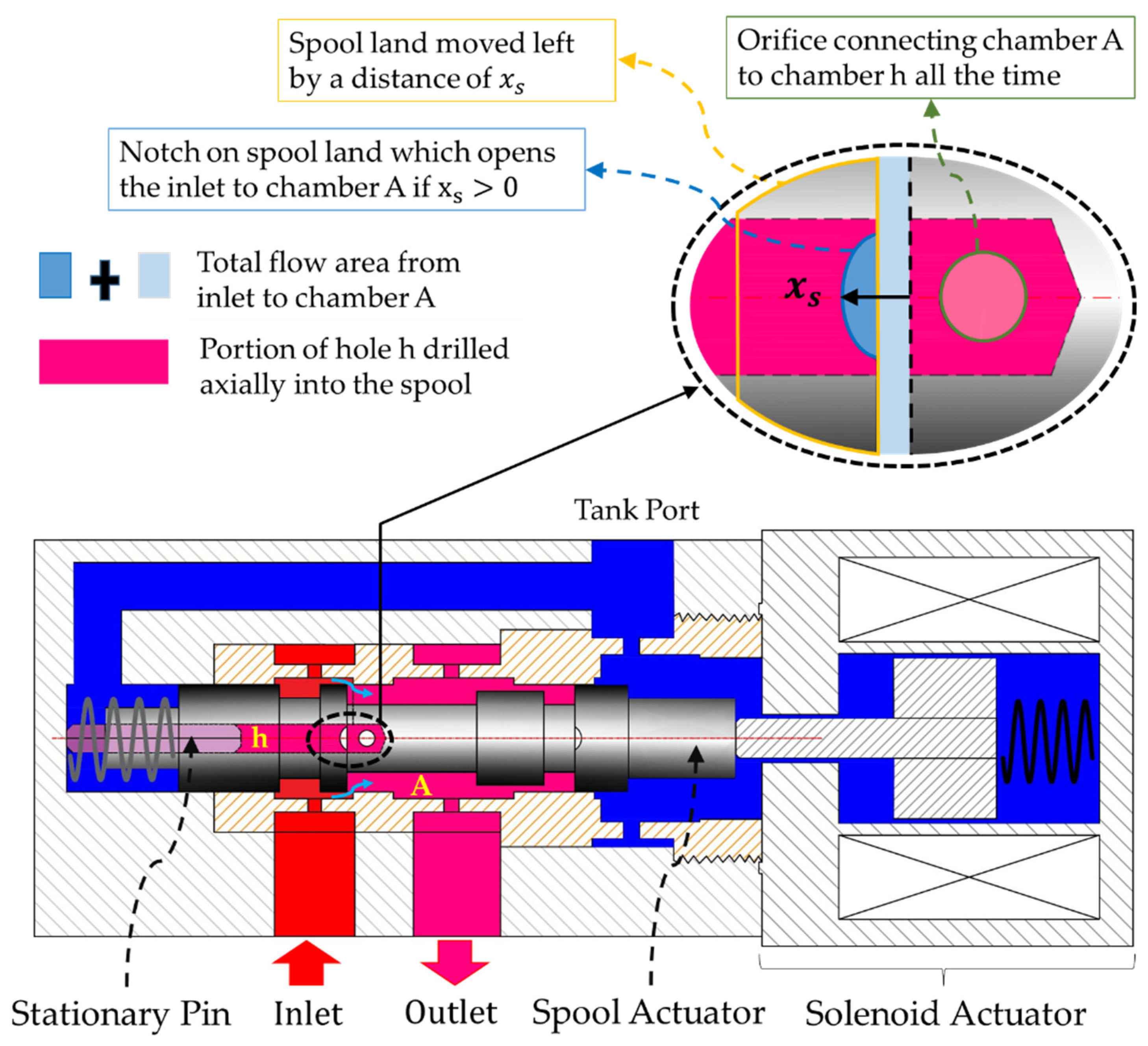
3.1. Details of the Valve Mechanism and Pin-Type Spool Actuator

The valve used in this study has a unique spool geometry, as shown in Figure 1c. A pin inside the spool actuator defines the pressure range for the valve. Similarly, the spool land’s outer diameter determines the flow area gradient with respect to the spool displacement. The spool edges contain circular notches. These details are shown in Figure 2.

3.2. Governing Equations

Equations (1)–(13) make a list of the governing equations applicable to the valve shown in Figure 2. The symbols are described in the nomenclature, and the parameters used are provided in

Table 1. Parameter values for valve mechanism used in this study.

Parameters	Values	Parameters	Values
$V_A$	$1122\times {10}^{-9} {\mathrm{m}}^3$	$R$	4 mm
$\beta$	$1.4 \left(\mathrm{GPa}\right)$	$r$	1 mm
$\rho$	$861 \mathrm{kg}/{\mathrm{m}}^3$	$k_1$	3000 N/m
$C_d$	0.62	$k_2$	1840 N/m
$C_v$	0.98	$m_s$	32 g
$Cos\theta$	$0.65, \mathrm{i}.\mathrm{e}., \theta ={50}^{°}$	$c_f$	80 Ns/m
$P_{in}$	50 bar (approximately)	$L_0$	9 mm
$A_0$	$\pi /4 \left({0.0006}^2\right) {\mathrm{m}}^2$	$L_1$	10 mm
$A_p$	$\pi /4 \left({0.00215}^2\right){ \mathrm{m}}^2$	$L_2$	8 mm

.

There are two chambers, Chamber A and Chamber h, as shown in Figure 2. Similar to any other control volume, as explained in detail by [21], the continuity equation for Chamber A is given by Equation (1).

$$Q_{in}=Q_{out}+Q_t+Q_h+\left(\frac{V_A}{\beta }\right)\frac{d{P}_A}{dt}$$

(1)

As already established in the previous studies [22], by treating the opening flow areas as orifices, the flow rates can be evaluated from the pressure difference, fluid density, discharge coefficient and the curtain areas as described by Equations (2)–(5).

Figure 3 shows a simplified version of Figure 2 and an overall placement of the valve in a hydraulic circuit.

$$Q_{in}=A_{1x}{C}_d\sqrt{\frac{2\left(P_{in}-P_A\right)}{\rho }}$$

(2)

$$Q_{out}=A_L{C}_d\sqrt{\frac{2\left(P_A-P_t\right)}{\rho }}$$

(3)

$$Q_t=A_{2x}{C}_d\sqrt{\frac{2\left(P_A-P_t\right)}{\rho }}$$

(4)

$$Q_h=A_0{C}_d\sqrt{\frac{2\left(P_A-P_h\right)}{\rho }}$$

(5)

As described in Appendix A, the curtain area of the spool as a function of the spool displacement is given by Equation (6).

$$A_{1x}=\begin{array}{c}0 ; x_s<0\mathrm{mm}\\ {\displaystyle \underset{0}{\overset{x_s}{\int }}6RSi{n}^{-1}\left(\frac{\sqrt{x_s\left(2r-x_s\right)}}{R}\right)d{x}_s ; 0\mathrm{mm}\le x_s<0.5\mathrm{mm}}\\ {\displaystyle \underset{0}{\overset{0.5\mathrm{mm}}{\int }}6RSi{n}^{-1}\left(\frac{\sqrt{x_s\left(2r-x_s\right)}}{R}\right)d{x}_s+2\pi R\left(x_s-0.5\mathrm{mm}\right); x_s\ge 0.5\mathrm{mm}}\end{array}$$

(6)

The curtain area connecting Chamber A to the tank is presented in Equation (7).

$$A_{2x}=\begin{array}{c}0 ; x_s>0\mathrm{mm}\\ {\displaystyle \underset{0}{\overset{-x_s}{\int }}6RSi{n}^{-1}\left(\frac{\sqrt{-x_s\left(2r+x_s\right)}}{R}\right)d{x}_s ; -0.5\mathrm{mm}<x_s\le 0\mathrm{mm}}\\ {\displaystyle \underset{0}{\overset{0.5\mathrm{mm}}{\int }}6RSi{n}^{-1}\left(\frac{\sqrt{-x_s\left(2r+x_s\right)}}{R}\right)d{x}_s+2\pi R\left(-x_s-0.5\mathrm{mm}\right); x_s<-0.5\mathrm{mm}}\end{array}$$

(7)

Similar to that for Chamber A, the continuity equation for Chamber h is described by Equation (8).

$$Q_h=Q_L-A_p{\dot{x}}_s+\frac{A_p\left(L_0-x_s\right)}{\beta }\frac{d{P}_h}{dt}$$

(8)

The leakage flow through the annular section between the spool and the pin is given by Equation (9), i.e., Hagen–Poiseuille equation [21].

$$Q_L=\frac{\left(P_h-P_t\right)\pi }{8l_c\rho \nu }\left[R_2{}^4-R_1{}^4-\frac{{\left(R_2{}^2-R_1{}^2\right)}^2}{\ln \left(\frac{R_2}{R_1}\right)}\right]$$

(9)

The forces exerted on the spool constitute the force balance equation that determines the spool’s motion.

$$m_s{\ddot{x}}_s+c_f{\dot{x}}_s+\left(k_1+k_2\right)x_s=F_{sol}-A_p{P}_h+F_{flow}$$

(10)

The solenoid force depends on the current in the solenoid coil. The flow force consists of transient and steady-state components, both of which are determined through the following equations well-established in previous studies [22].

$$F_{flow}=F_{st}+F_{tr}$$

(11)

$$F_{st}=-2C_d{C}_v{A}_{1x}\left(P_{in}-P_A\right)cos\theta +2C_d{C}_v{A}_{2x}\left(P_A-P_t\right)cos\theta$$

(12)

$$F_{tr}=L_1{C}_d\frac{d{A}_{1x}}{d{x}_s}\sqrt{2\rho \left(P_{in}-P_A\right)}\frac{d{x}_s}{dt}+L_2{C}_d\frac{d{A}_{2x}}{d{x}_s}\sqrt{2\rho \left(P_A-P_t\right)}\frac{d{x}_s}{dt}$$

(13)

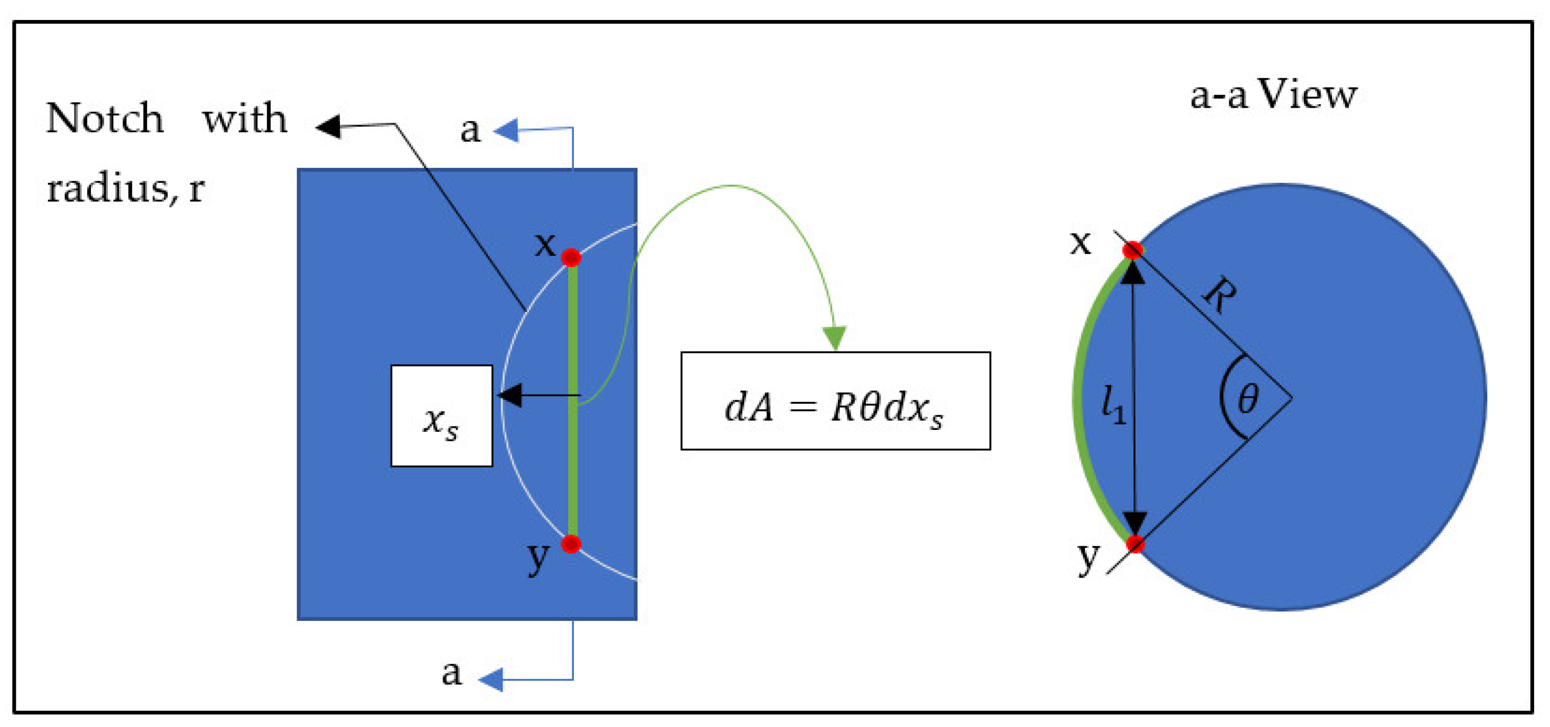
3.3. Assumptions and Simplification

• Initially, the spool position is centered, i.e., $x_s=0$.
• As reflected in Equation (6), leakage flow through the pin-spool clearance is assumed to be fully developed and laminar due to its high length to cross-section ratio and small fluid velocity justified later through results.
• Temperature variations are ignored, and an operating temperature of 25 °C is used for the determination of oil properties.
• HLP-46 is used as the working fluid.
• All the edges are assumed to be perfectly sharp.
• The spool lands are perfectly round in shape with circular notches on each edge.
• The spatial pressure variation in Chamber A or Chamber h is negligible.
• Inlet pressure is assumed to be the same as that of the actual piston pump.
• The ratio of spool displacement to spool-sleeve clearance was assumed to be close to 1 in order to be consistent with the details given in Section 3.4.

3.4. Actual Valve Model Parameters

The valve, as well as the working fluid used in this study, has specifications or features described in Table 1. Some of these values are related to the assumptions, and others are based on details that can be materialized.

As reported in [22] (p. 103), the cosine of the actual jet angle ($Cos\theta$) lies between 0.36 and 0.94, so it is reasonable to use the average value, i.e., 0.65, in the mathematical model.

It is obvious from previous studies that a discharge coefficient of 0.61 corresponds to a sharp-edged orifice [22]. Furthermore, we consider that the sleeve and spool are well machined, and the flow area that is opened due to the spool movement well resembles an orifice that has sharp edges.

The values of all the parameters shown in Table 1 are used to determine the solution of the mathematical model already formulated earlier.

4. Modeling Using Simulink

In this work, all the equations are kept in the time domain without any linearization, which makes the approximation more accurate and reliable as opposed to other studies that perform linearization before solving the mathematical model.

The model was to be numerically solved using Simulink. For this purpose, Runge–Kutta methods are very popular for solving a system of ordinary differential equations. One example, i.e., the Runge–Kutta method of order 4 (RK4), is described below.

$$\frac{dy}{dt}=f\left(t,y\right), y\left(t_0\right)=y_0$$

(14)

$$y_{n+1}=y_n+\frac{1}{6}h\left(k_1+2k_2+2k_3+k_4\right)$$

(15)

$$t_{n+1}=t_n+h$$

(16)

$$k_1=f\left(t_n,y_n\right), k_2=f\left(t_n+\frac{h}{2},y_n+h\frac{k_1}{2}\right)$$

(17)

$$k_3=f\left(t_n+\frac{h}{2},y_n+h\frac{k_2}{2}\right), k_4=f\left(t_n+h,y_n+h{k}_3\right)$$

(18)

If Equation (14) is the initial value problem, then an iterative method with the next point computed through Equations (15)–(18) can be used to arrive at the time domain solution to the initial value problem. The order of the Runge–Kutta method can be increased if more accuracy is needed, but it will increase the computation cost. In this study, the Runge–Kutta method of order 5 was implemented by using the ODE45 solver.

In Simulink, the dynamics of the valve-spool actuator are modeled with the help of governing equations (Equations (1)–(13)). The criteria for selecting the solver were based on accuracy and speed because the model consists of non-linear ordinary differential equations in the time domain. As per [23], ODE45 has medium accuracy as compared to other solver types. Furthermore, according to [24,25,26], the solver ODE45 has a truncation error that depends on the step size. The smaller the step size, the more accurate the solution would be. However, if the step size is too small, the solution time may increase to an undesirable value. Thus, ODE45, with a variable step size, was chosen to be a suitable solver for the Simulink model.

5. Experimental Results for Use in Simulation

In order to determine the solution to the mathematical model through the ODE solver in Simulink, inlet pressure data and solenoid force data were essential, which were obtained through experimentations.

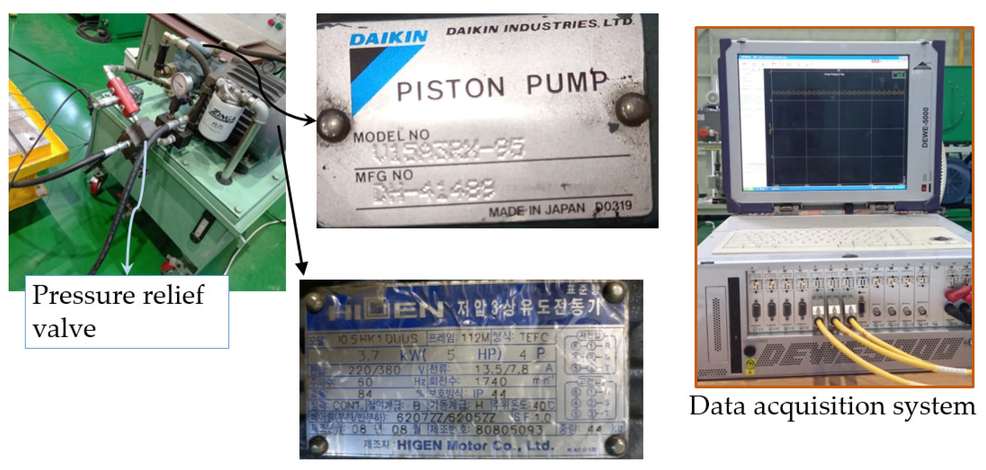
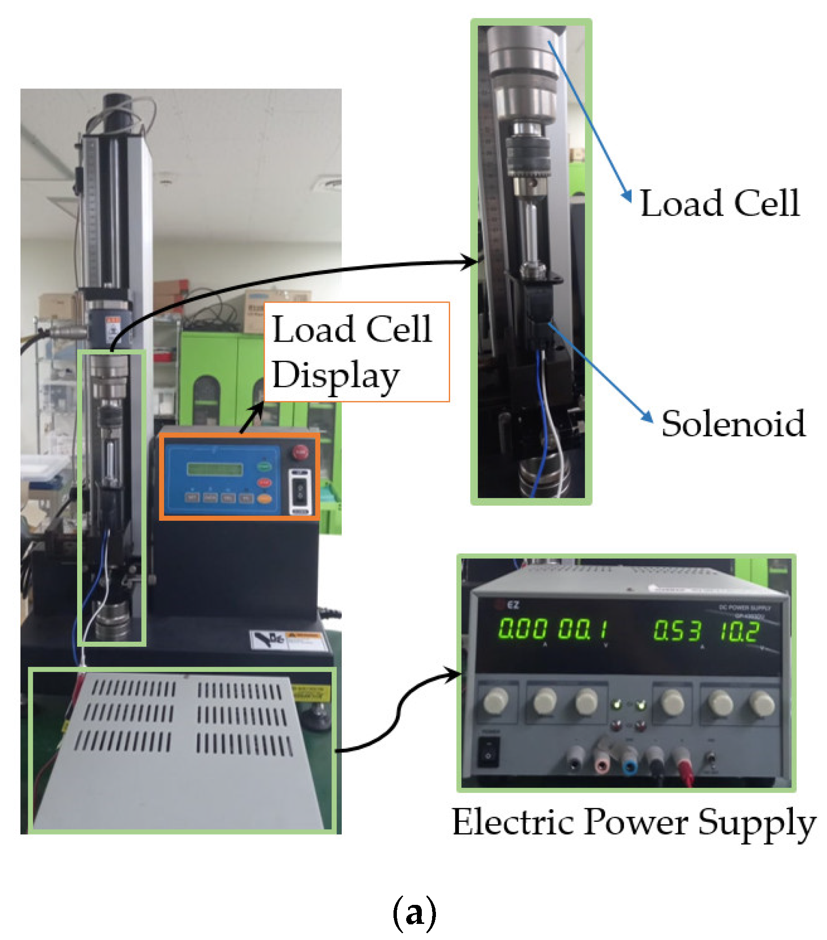
5.1. Test Setup for Pump Pressure Measurement

The hydraulic pump with an inlet connected to a hydraulic tank and outlet connected to a pressure transducer was turned on with the pressure controlled through a pilot-operated pressure relief valve. Pressure settings in the range of 40–90 bar were considered. The pressure transducer installed at the pump outlet was connected to a data acquisition system to gather the pressure versus time data for use in the simulation. The pump used was manufactured by DAIKIN (model no V15A3AX-95). All these details can be seen in Figure 4.

The pressure transducer was connected to the data acquisition system. The sampling rate was kept at 10 kHz, which reduces the error significantly. The specifications of the pressure transducer are shown in

Table 2. Pressure transducer specifications.

Model	PCH-100K	Safe Over Load	150% of Rated Current
Capacity	100 bar	Non-linearity	0.2% of rated output
Rated Output	1.503 mV/V	Hysteresis	0.2% of rated output

.

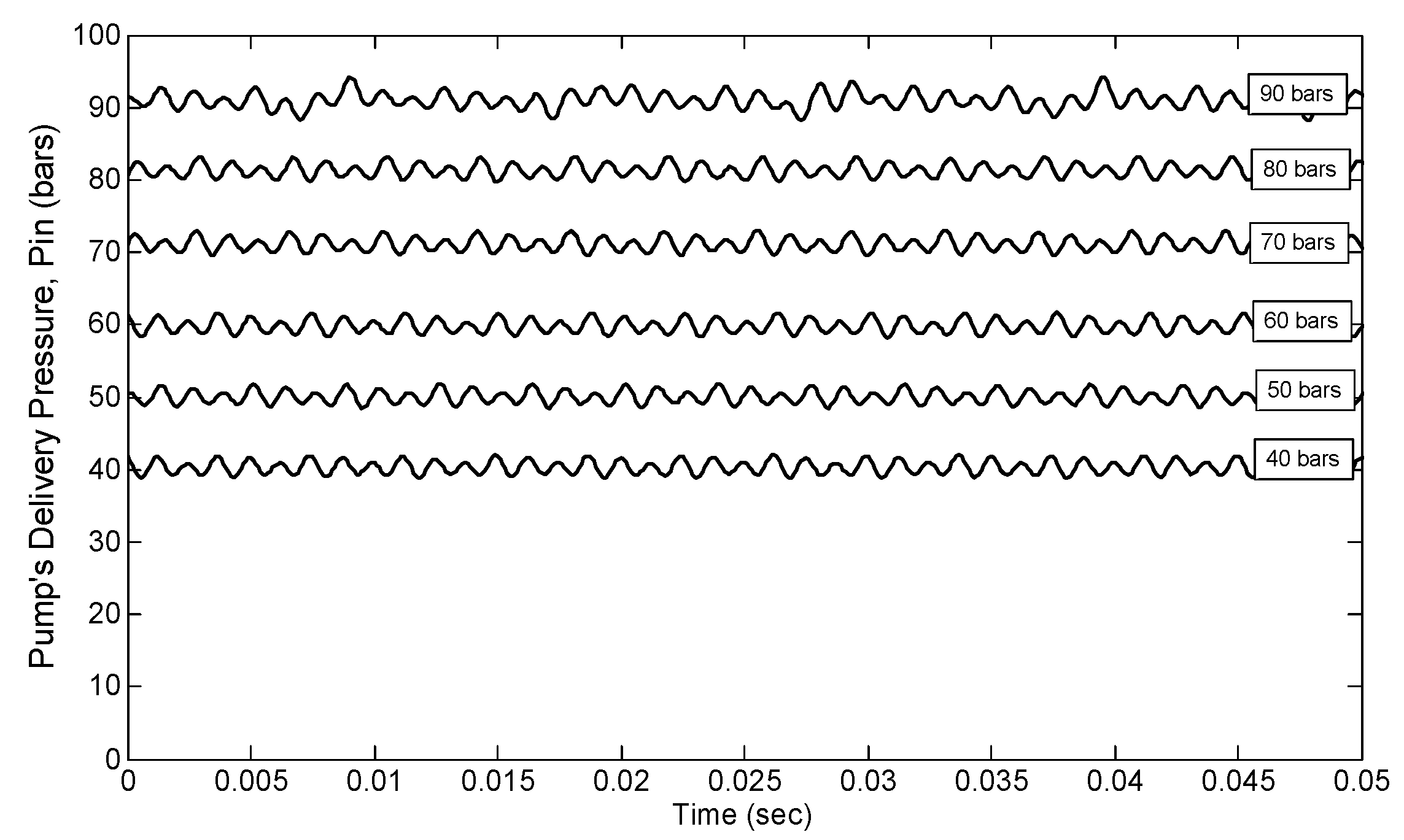
5.2. Pump Pressure Results

While keeping the pressure settings at x bar with the help of a pressure relief valve, the exact pressure vs. time curve as recorded by the data acquisition system is shown in Figure 5.

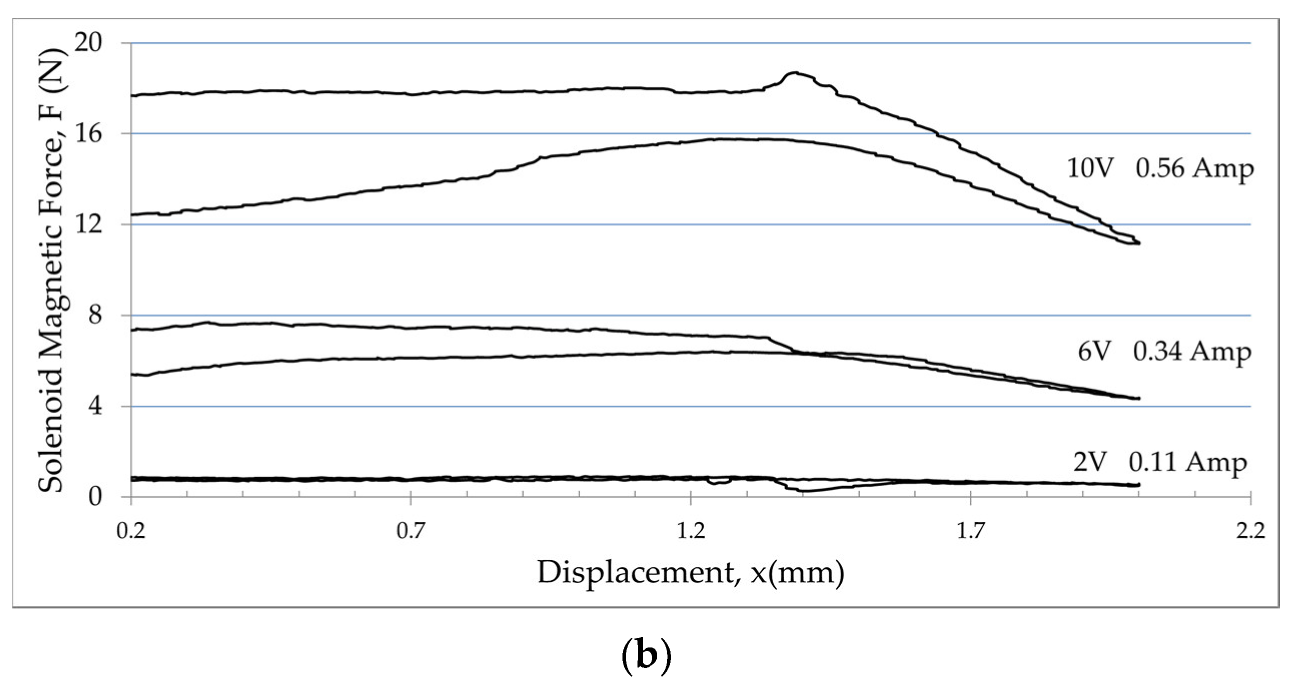
5.3. Solenoid Force Measurement

The solenoid force acting on the spool actuator was determined through experiments as well. The relationship between the solenoid current and the resulting force was determined through a load cell, as shown in Figure 6. The power rating of the solenoid for which the valve is modeled was 20 watts.

Figure 6b shows that the maximum solenoid force can be estimated at 17 N, which is why it was decided to use the solenoid force lower than 17 N when running the Simulink model. The sensor specifications are shown in

Table 3. Specifications of load cell used for measuring the actuating force.

Model	LRM-100N	Safe Over Load	120% of Rated Current
Capacity	100 N	Non-linearity	0.05% of rated output
Rated Output	1.5 mV/V	Hysteresis	0.05% of rated output

.

6. Simulation Results and Discussion

After setting up the mathematical model in Simulink, the model was run for different values of design and operational parameters. The default values were based on an earlier design of the valve developed in the laboratory.

6.1. No Load-Flow Condition

To simulate a situation where the valve outlet is blocked, it is necessary to know how the outlet pressure responds when the outlet orifice diameter is zero, and as we discover later, the output pressure keeps on fluctuating without converging to a single value. One way to reduce that fluctuation would be to increase the Coulomb friction, but that would generate or worsen the heat losses, contribute to wear and reduce the life of the spool actuator, which is the reason why the friction coefficient was kept constant in this study. Other potential factors involved in the achievement of such a feat include the inlet pressure, the solenoid force and the pin dimensions.

A study on a no-load flow condition by [16] takes into account the piping as well as the pressure-reducing valve and determines how the valve output behaves experimentally when the pressure at the valve outlet is varied. However, in this study, keeping the focus on the valve only, we consider how the valve responds when the actuating force is applied to the valve and the valve outlet is blocked, while applying a pulsating inlet pressure to the valve.

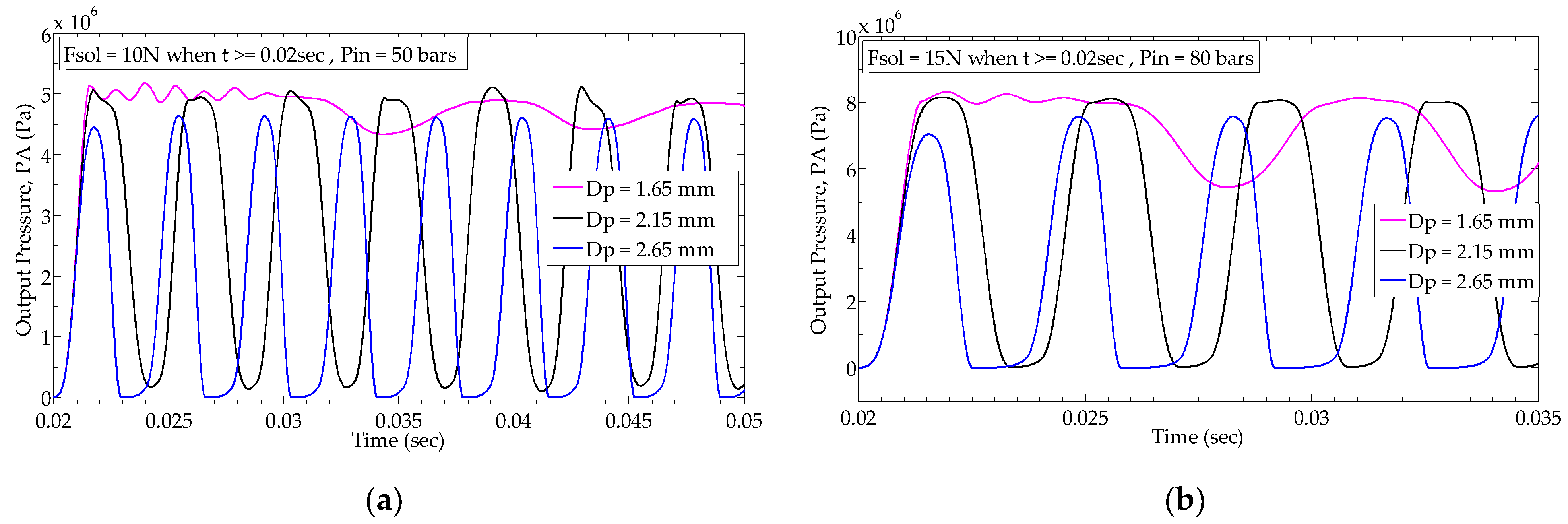
6.1.1. Criteria for Selection of Inlet Pressure and Pin Diameter

For a pressure-reducing valve, the inlet pressure should be greater than the intended steady-state pressure at the outlet. The pin diameter influences the range of steady-state output pressure for a specific range of solenoid force. Under a no-load flow condition, if the range of force exerted by the solenoid actuator is fixed, i.e., 0 or 15 N, as considered in this study, the pressure range can be derived from Equation (10), as shown in Equation (19).

$$P_{A,ss}=\frac{F_{sol}}{\pi \left(\frac{D_p{}^2}{4}\right)}$$

(19)

The inlet pressure is to be selected so that it is greater than $P_{A,ss}$, set by the solenoid force given in

Table 4. Pressure output and solenoid force as related to suitable inlet pressure settings.

${\mathit{F}}_{\mathit{s}\mathit{o}\mathit{l}}$	${\mathit{D}}_{\mathit{p}}$	${\mathit{P}}_{\mathit{A},\mathit{s}\mathit{s}}$	$\mathbf{Suitable} {\mathit{P}}_{\mathit{i}\mathit{n}}{ }^1$
10 N	1.65 mm	46.8 bar	50 bar or greater
	2.15 mm	27.5 bar	30 bar or greater
	2.65 mm	18.1 bar	20 bar or greater
15 N	1.65 mm	70.2 bar	70 bar or greater
	2.15 mm	41.3 bar	50 bar or greater
	2.65 mm	27.2 bar	30 bar or greater

¹ We considered 40 to 80 bar pressure settings only.

.

6.1.2. Influence of Pin Diameter and Inlet Pressure on Outlet Pressure

The Simulink model was run for different values of pin diameter and inlet pressure without violating the criteria shown in Table 4. The output pressure is plotted with time, as shown in Figure 7 and Figure 8.

For cases depicted in Figure 7 and Figure 8, as the pin diameter is increased, the fluctuations in the output pressure increase significantly. This is because the pin exposes the spool actuator to an unbalanced hydraulic force that is proportional to the pin’s cross-sectional area. If higher forces are involved due to increased pin diameter, the fluctuations, already exacerbated by the presence of the fluctuations in the inlet pressure, would worsen. The presence of fluctuations in the inlet pressure combined with the increase in hydraulic force contributes to such an outcome.

The inlet pressure fluctuations, as expressed in Figure 5, depend on the pump operation technique. The pump involved in this study is a piston pump that relies on a number of reciprocating cylinders to build and deliver pressure. In any type of pump, the delivery pressure cannot be perfectly maintained at a constant value. Numerous studies on pressure pulsations in hydraulic pumps show that such a phenomenon should not be ignored when solving the mathematical model [27,28,29]. This factor is thus taken into account by providing the pump test data to the Simulink model in order to create realistic input conditions for simulation. The details of how the test data were obtained through experiments are shown in Figure 4 and Figure 5.

Knowing about the impact of pin diameter and analyzing the subsequent results are necessary when designing a valve for an application such as variable displacement pumps. Furthermore, the resulting fluctuations in the valve outlet pressure will result in increased noise and reduced reliability of the pump, as well as inaccuracies in the pumps outlet pressure or flow rate due to hydraulic shocks, examples of which can be seen in [30,31,32,33]. For any particular application, the effect of pin diameter is to be carefully considered, especially for a no-load flow condition. The valve should be able to handle the inlet pressure changes even after being subjected to a drastic change in the actuating force.

Considering the case of Dp = 1.65 mm, Table 4 shows that for 10 and 15 N, the suitable pressure settings are 50 and 80 bar, respectively. If the inlet pressure is set close to the suitable pressure (as is done for the cases of Figure 7a,b), the fluctuations are less profound and similar to each other, shown by the magenta colored line in Figure 7. However, if the inlet pressure is increased to 80 bar for 10 N when only 50 bar is sufficient, the output pressure starts to deviate more significantly, and variations are more profound without being able to die down as time proceeds.

If the simulation is performed with no-load flow condition, the output pressure is oscillatory and does not converge to a single point. Similar behavior of a pressure-reducing valve was also reported and investigated by [13,34]. Consequently, valve stability becomes very crucial at low flow conditions. Several studies related to valve stability and chaos in a hydraulic system were conducted by different researchers reinforcing the significance of implications arising from such oscillatory responses [35,36,37,38,39].

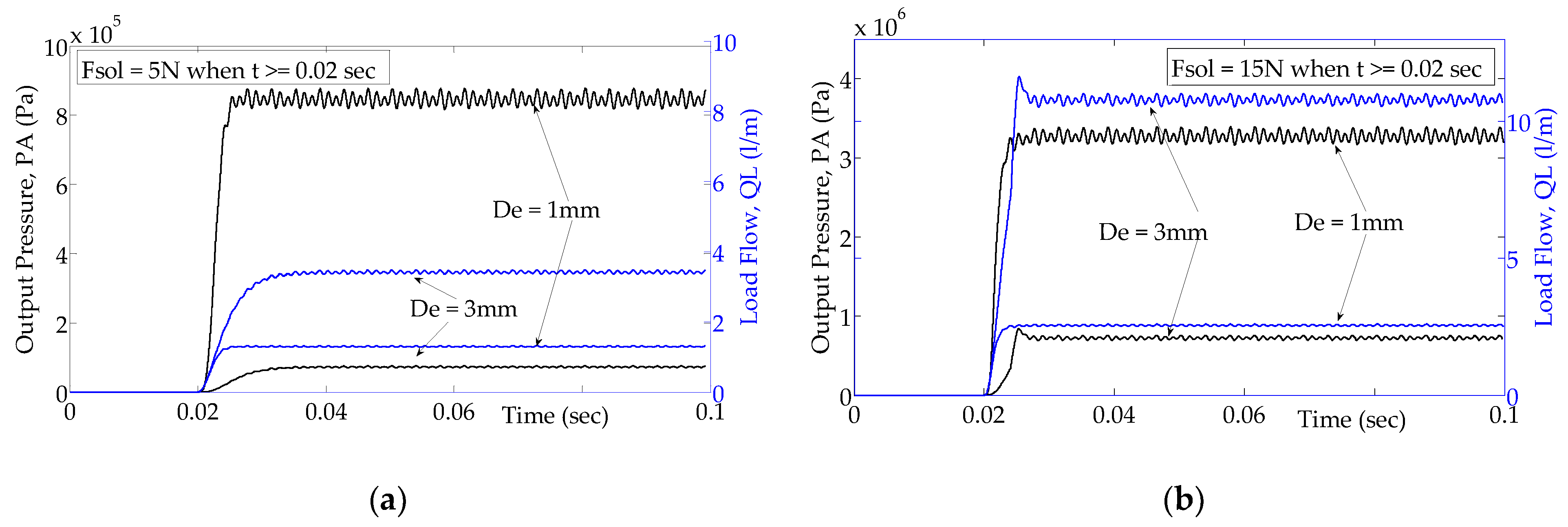
6.2. Results with Opened Outlet

To simulate the opening of a valve outlet, the diameter of the outlet orifice, De, was varied, and the Simulink model was solved thereafter. For steady-state analysis, the pin diameter was fixed at 2.15 mm, so an inlet pressure setting of 50 bar was chosen, which conforms to the criterion established in Table 4.

6.2.1. Steady-State Results

The steady-state values of outlet pressure and the load flow rates obtained after running the Simulink model for different values of solenoid force and outlet orifice diameter are mapped and summarized in Figure 9.

Because of fluctuations created due to the input pressure, as shown in Figure 5, the averages of steady-state values were used to get the data points in Figure 9. It is clear that an increase in the solenoid force lifts the pressure-flow curve of the valve upward. So, if the user needs a higher range of flow rate as well as pressure, a higher value of solenoid force would be needed. In this study, the solenoid used has a maximum available actuating force of 17 N, as determined from the experimental results shown in Figure 6.

With an increase in the diameter of the outlet orifice, i.e., De, from 0 to 3 mm, the pressure-flow curve is affected significantly, but a further change after 4 mm does not affect the steady-state pressure or flow rate. It means that a 4 mm orifice size at the outlet means the valve is fully opened, and any further change in flow rate or pressure is not possible by changing the size of the outlet orifice. This is due to the fact that the inlet pressure that drives the flow into the valve is constant, and although the outlet opening is increased, the pressure drop cannot increase accordingly, which puts a limit on the maximum possible flow for the valve. The valve studied in this study was designed for a flow rate of 10 L/min, which was achieved successfully.

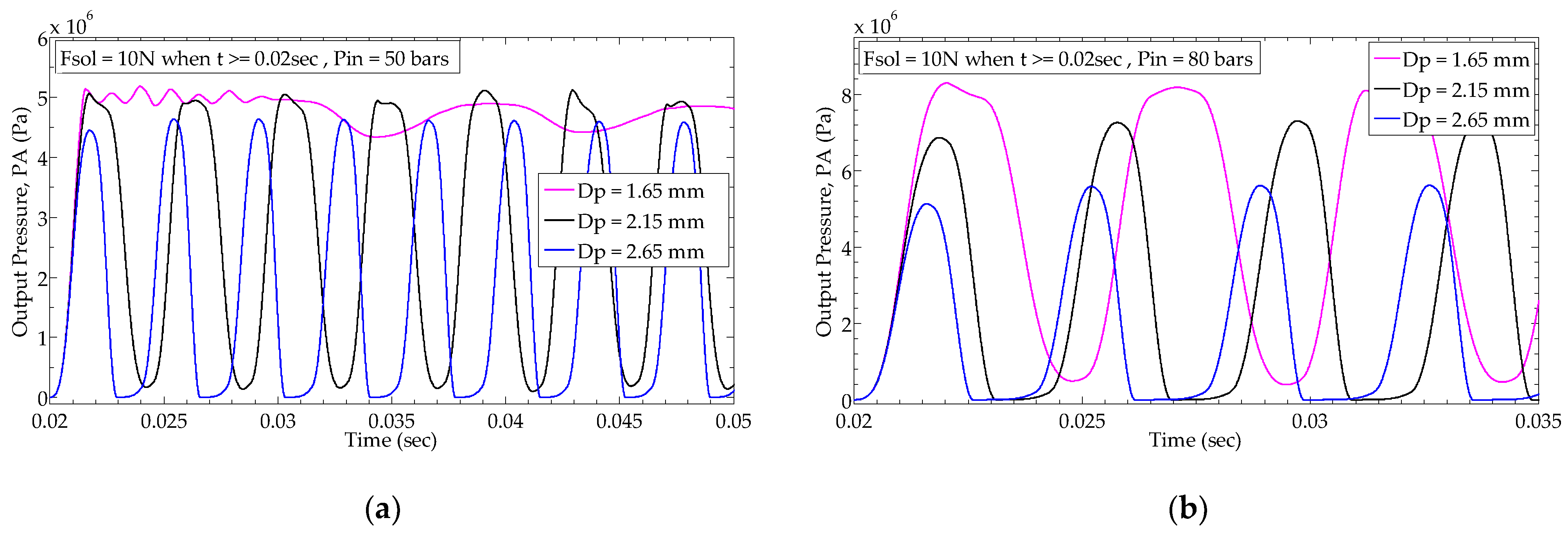
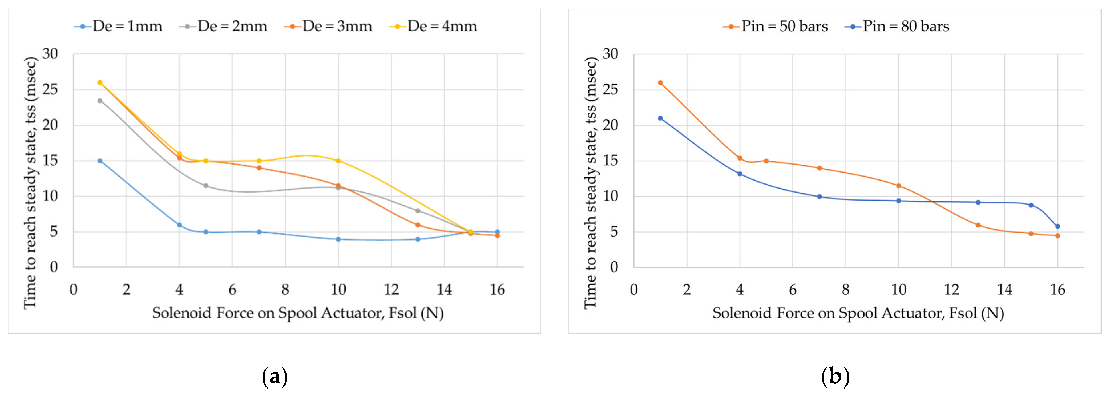
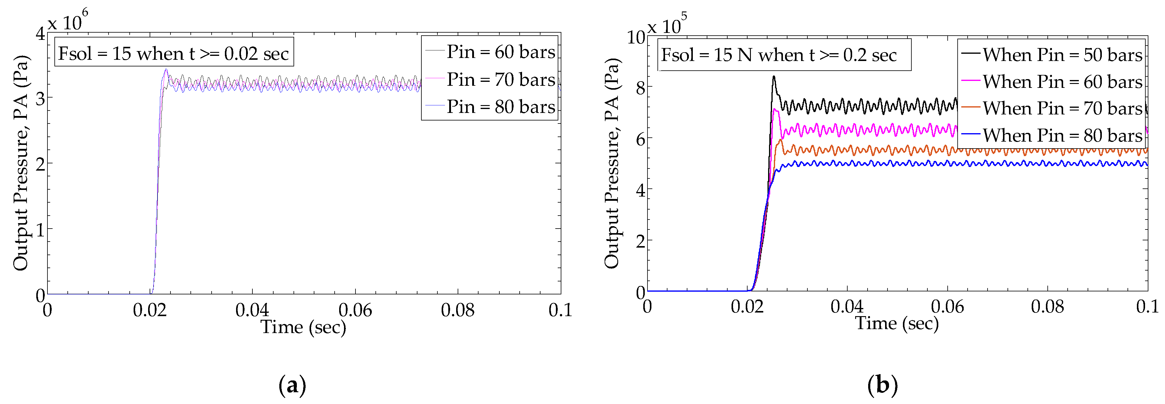
6.2.2. Step Response Results for Different Valve Openings and Inlet Pressure Settings

A step input of the solenoid force was applied to the spool actuator at t = 0.02 s. The resulting output pressure was recorded as discussed in the following.

Figure 10 shows the output pressure for two different sizes of outlet orifice, i.e., 1 and 3 mm. These two diameters were selected because they significantly affect the response, as evident from Figure 9. Furthermore, solenoid forces of 5 and 15 N were used to demonstrate the effect of solenoid force on the transient response of the valve. Many such cases were analyzed, whose summary is plotted in Figure 9.

If the valve’s outlet orifice diameter is 3 mm, the steady-state flow rate reaches 11 L/min, while the pressure output settles at 7 bar, as shown in Figure 10. An increase in the outlet diameter creates an overshoot in the outlet pressure, which is due to the inertia of the spool amid acceleration resulting from higher solenoid force combined with an opened outlet allowing more flow to go out of Chamber A, ultimately resulting in overspeeding of the spool actuator to compensate for the flow going out of Chamber A.

To measure how fast the valve responds to the solenoid force, the time taken to reach the steady-state value (i.e., rising time) was determined. The speed with which the pressure output responds after applying a step input to the spool depends on the magnitude of the solenoid force, as well as the inlet pressure, as shown in Figure 11. For a certain outlet orifice size, the response gets quicker with an increase in the solenoid force. However, at the maximum value of solenoid force, i.e., 16 N, the response time for all the outlet orifice sizes converges to a single value, as shown in Figure 11. For smaller solenoid forces, the valve is slow to respond because the acceleration produced by the net force on the spool actuator is not strong enough to produce enough acceleration in the spool actuator. At low solenoid forces, the difference among the rising times for different outlet orifice sizes are significant, but at 15 or 16 N, all the outlet sizes respond with the same speed. This is because higher solenoid force makes other factors more important as the flow force as well as feedback force grow stronger in magnitude, making the solenoid force not as influential as at lower values. Figure 11 shows the rising times vs. solenoid force for two different settings of inlet pressure, i.e., 50 and 80 bar, for an outlet orifice of 3 mm.

As shown in Figure 12, for small flow rates, e.g., when De =1 mm, as the inlet pressure is increased, the valve responds almost similarly because flow forces are insignificant at smaller flow rates. However, as the valve outlet is opened more, e.g., when De = 3 mm, the increase in inlet pressure results in a smaller outlet pressure, this is a consequence of the combined influence that the steady-state force, as well as the pressure drop across the valve inlet, has on the dynamics of the spool actuator and the valve. At high flow rates, the inlet pressure influences the response more compared to smaller flow rates. For these results, the solenoid force of 15 N was applied as a step input at t = 0.02 s.

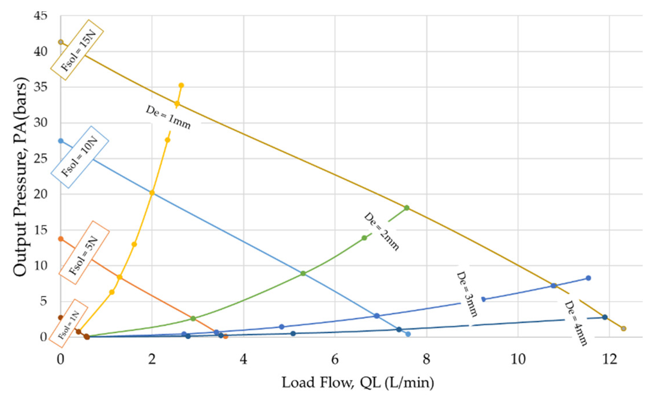
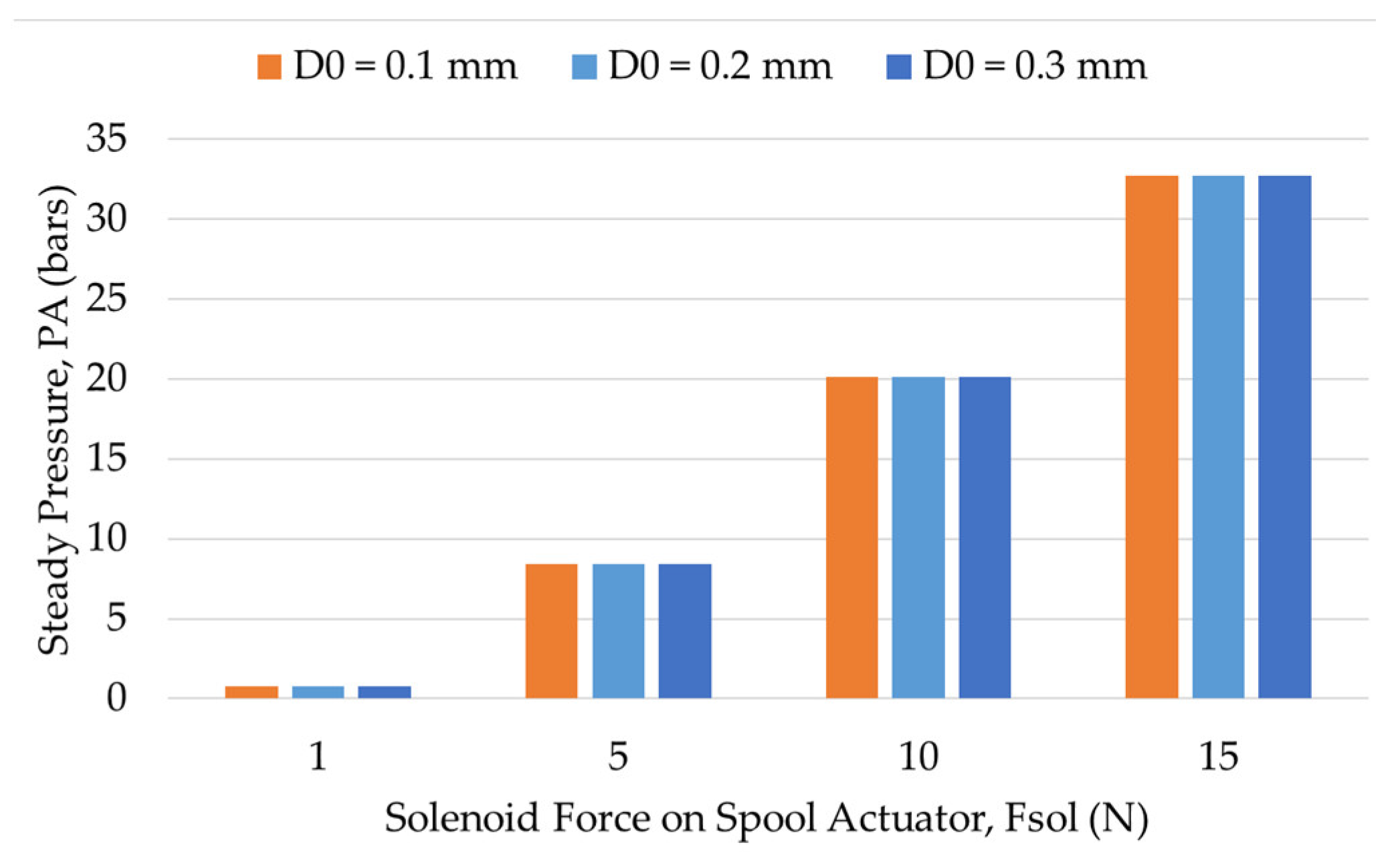
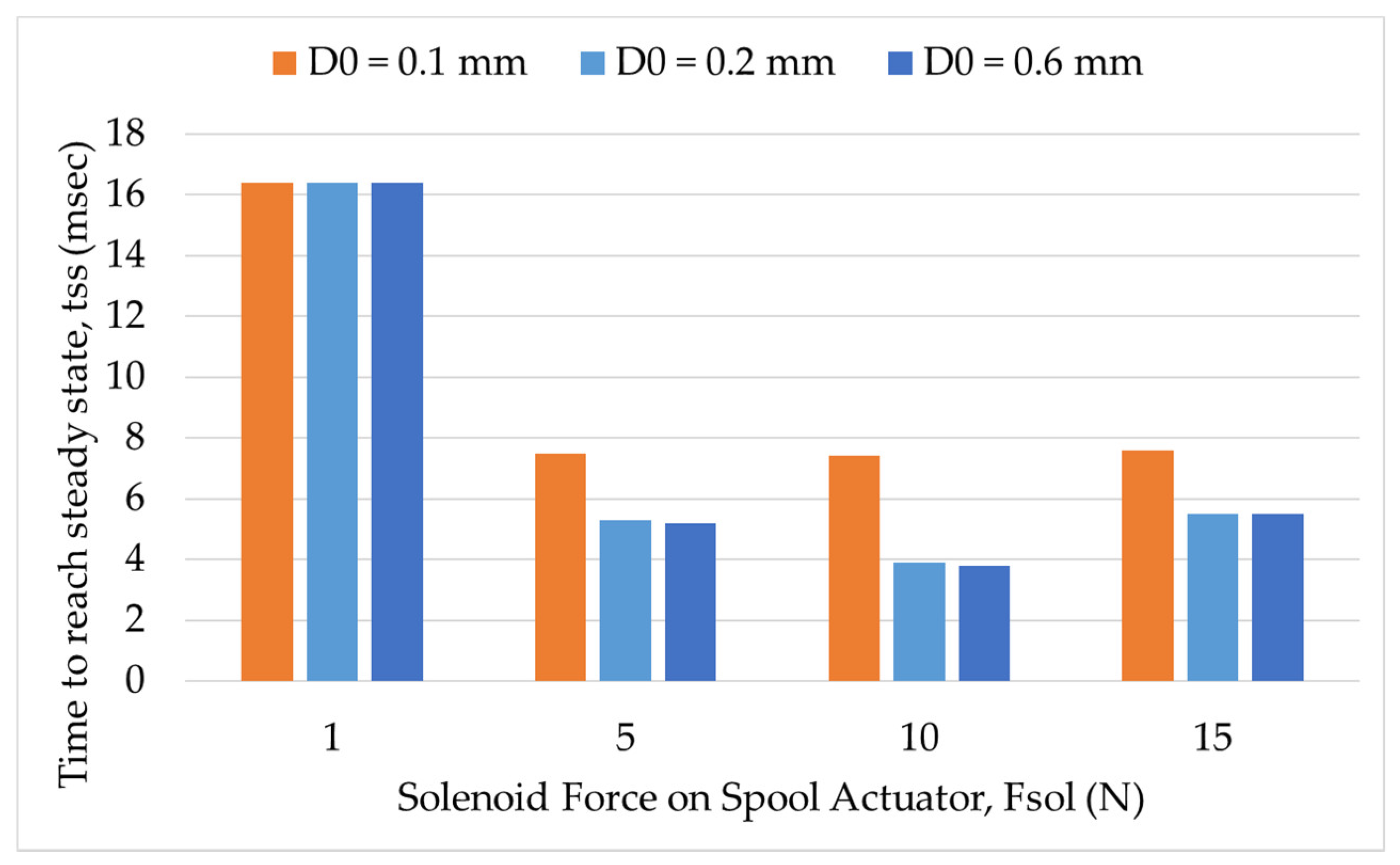
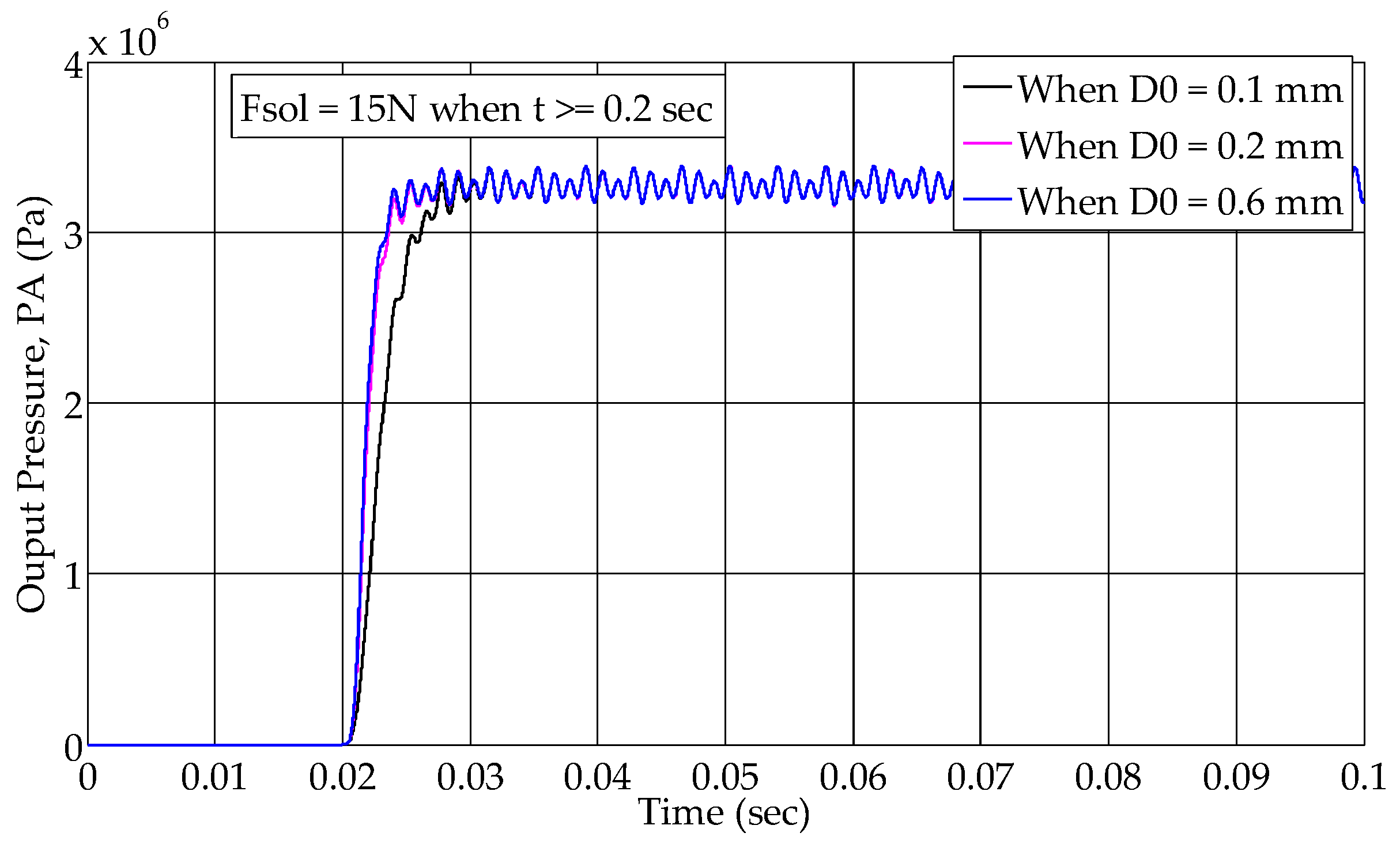
6.2.3. Influence of Damping Orifice on Output

Orifices can be used as dampers in many hydraulic components [40,41].

As shown in Figure 13 and Figure 14, we found out that the spool actuator can be damped by manipulating the orifice size, D0, that connects Chamber A with Chamber h. The orifice size does not affect the steady-state pressure. The transient results in Figure 14 indicate that reducing the orifice size slows down the response of the valve, as summarized in Figure 15 for different values of actuating solenoid force. This is because a smaller orifice allows less flow rate, making the response of pressure in Chamber h to pressure, PA, slower.

The diameter of 0.6 mm can be deemed suitable, as it results in a faster response and is easy to manufacture. If the orifice size is reduced even more, it would make its manufacturing more difficult, the valve prone to dirt and the spool actuator slower to respond.

7. Conclusions

The pressure-reducing mechanism investigated in this study was modeled through governing equations in Simulink. A solver based on Runge–Kutta method of differential equations solutions, i.e., ODE45, was used to carry out the simulation for different design and operational parameters. The influence of such parameters is examined and summarized in this work. We found that if the valve outlet is blocked, the spool produces a fluctuating output pressure, which was expected as reported in earlier studies. The fact that inlet pressure has to be higher than the intended steady-state outlet pressure was used as a criterion for pin diameter on the basis of solenoid force and inlet set pressure. As a result, a pin diameter of 2.15 mm was selected for achieving a reduced pressure of 0–41 bar for a 50 bar inlet pressure setting.

For an opened outlet, when the inlet pressure setting is changed, it is found that flow force is the most significant parameter. It is clear from the transient as well as steady-state responses for cases where the outlet orifice size is increased.

The rising time of output pressure turned out to be less than 20 ms for a solenoid force of 5 N or greater, which is suitable for use in many hydraulic applications. The damping orifice is found to influence the transient response only if the diameter is close to 0.1 mm, which means that we can change the orifice size without affecting the valve response if the diameter is 0.2 mm or above.

With the help of deductions drawn from this research work, it is possible to design a similar pin-type pressure-reducing valve for a certain application that consists of a spool actuator and a solenoid with a known force output. The only problem in this design is the instability of output pressure when the flow is blocked at the outlet, which can be handled through further study as to how to use a solenoid control in bringing such instabilities down.

References

1. Slama, V.; Mrozek, L.; Tajc, L.; Klimko, M.; Zitek, P. Flow Analysis in a Steam Turbine Control Valve with Through-Flow Valve Chamber. J. Nucl. Eng. Radiat. Sci. 2021, 7, 1–7. [Google Scholar] [CrossRef]
2. Wu, D.; Li, S.; Wu, P. CFD simulation of flow-pressure characteristics of a pressure control valve for automotive fuel supply system. Energy Convers. Manag. 2015, 101, 658–665. [Google Scholar] [CrossRef]
3. Frosina, E.; Senatore, A.; Buono, D.; Stelson, K.A. A Modeling Approach to Study the Fluid-Dynamic Forces Acting on the Spool of a Flow Control Valve. J. Fluids Eng. 2017, 139, 1–11. [Google Scholar] [CrossRef] [Green Version]
4. Pérez-Sánchez, M.; López-Jiménez, A.P.; Ramos, M.H. PATs operating in water networks under unsteady flow conditions: Control valve manoeuvre and overspeed effect. J. Water (Switzerland) 2018, 10, 529. [Google Scholar] [CrossRef] [Green Version]
5. Xu, B.; Cheng, M. Motion control of multi-actuator hydraulic systems for mobile machineries: Recent advancements and future trends. Front. Mech. Eng. 2017, 13, 151–166. [Google Scholar] [CrossRef]
6. Fang, X.; Ouyang, X.; Yang, H. Investigation into the Effects of the Variable Displacement Mechanism on Swash Plate Oscillation in High-Speed Piston Pumps. Appl. Sci. 2018, 8, 658. [Google Scholar] [CrossRef] [Green Version]
7. Jung, D.-S.; Kim, H.-E.; Kang, E.-S. Multi-function Control of Hydraulic Variable Displacement Pump with EPPR Valve. Trans. Korean Soc. Automot. Eng. 2006, 14, 160–170. [Google Scholar]
8. Jin, Z.-J.; Chen, F.-Q.; Qian, J.-Y.; Zhang, M.; Chen, L.-L.; Wang, F.; Fei, Y. Numerical analysis of flow and temperature characteristics in a high multi-stage pressure reducing valve for hydrogen refueling station. Int. J. Hydrogen Energy 2016, 41, 5559–5570. [Google Scholar] [CrossRef]
9. Chao, Q.; Zhang, J.; Xu, B.; Huang, H.; Pan, M. A Review of High-Speed Electro-Hydrostatic Actuator Pumps in Aerospace Ap-plications: Challenges and Solutions. J. Mech. Des. Trans. ASME 2019, 141, 1–13. [Google Scholar] [CrossRef] [Green Version]
10. Carravetta, A.; Chacon, C.M.; Fecarotta, O.; McNabola, A.; Ramos, M.H. Chapter 13—Energy harvesting in water supply systems. In Sustainable Water Engineering; Charlesworth, S., Booth, C., Adeyeye, K., Eds.; Elsevier: Amsterdam, The Netherlands, 2020; pp. 229–254. [Google Scholar]
11. Balau, A.E.; Caruntu, C.F.; Patrascu, D.I.; Lazar, C.; Matcovschi, M.H.; Pastravanu, O.; Lazǎr, C. Modeling of a pressure reducing valve actuator for automotive applications. In Proceedings of the 2009 IEEE International Conference on Control Applications, Saint Petersburg, Russia, 8–10 July 2009; pp. 1356–1361. [Google Scholar]
12. He, X.; Zhao, D.; Sun, X.; Zhu, B. Theoretical and Experimental Research on a Three-Way Water Hydraulic Pressure Reducing Valve. J. Press. Vessel. Technol. 2017, 139, 1–9. [Google Scholar] [CrossRef]
13. Janus, T.; Ulanicki, B. Improving Stability of Electronically Controlled Pressure-Reducing Valves through Gain Compensation. J. Hydraul. Eng. 2018, 144, 1–13. [Google Scholar] [CrossRef]
14. Ulanicki, B.; Skworcow, P. Why PRVs Tends to Oscillate at Low Flows. Procedia Eng. 2014, 89, 378–385. [Google Scholar] [CrossRef] [Green Version]
15. Prescott, S.L.; Ulanicki, B. Dynamic Modeling of Pressure Reducing Valves. J. Hydraul. Eng. 2003, 129, 804–812. [Google Scholar] [CrossRef]
16. Meniconi, S.; Brunone, B.; Mazzetti, E.; Laucelli, D.B.; Borta, G. Hydraulic characterization and transient response of pressure reducing valves: Laboratory experiments. J. Hydroinform. 2017, 19, 798–810. [Google Scholar] [CrossRef]
17. Aung, Z.N.; Peng, J.; Li, S. Reducing the steady flow force acting on the spool by using a simple jet-guiding groove. In Proceedings of the 2015 International Conference on Fluid Power and Mechatronics (FPM), Harbin, China, 5–7 August 2015; pp. 289–294. [Google Scholar]
18. Stone, J.A. Discharge Coefficients and Steady-State Flow Forces for Hydraulic Poppet Valves. J. Basic Eng. 1960, 82, 144–154. [Google Scholar] [CrossRef]
19. Yun, S.-N.; Lee, Y.-L.; Khan, H.A.; Kang, C.-N.; Ham, Y.-B.; Park, J.-H. Proportional Flow Control Valve for Construction Vehicle. In Proceedings of the 2019 23rd International Conference on Mechatronics Technology (ICMT), Salerno, Italy, 23–26 October 2019; pp. 1–3. [Google Scholar]
20. Khan, H.A.; Yun, S.-N. Modeling and Simulation of an EPPR Valve Coupled with a Spool Valve. J. Drive Control 2019, 16, 30–35. [Google Scholar]
21. Munson, R.B.; Young, F.D. Fundamentals of Fluid Mechanics; John Wiley & Sons, Inc.: Hoboken, NJ, USA, 2015. [Google Scholar]
22. Merritt, E.H. Hydraulic Control Systems; John Wiley & Sons, Inc.: Hoboken, NJ, USA, 1967. [Google Scholar]
23. Choose an ODE Solver. Available online: https://www.mathworks.com/help/matlab/math/choose-an-ode-solver.html#bu7wegm-1 (accessed on 1 August 2021).
24. Baker, T.; Dormand, J.; Gilmore, J.; Prince, P. Continuous approximation with embedded Runge-Kutta methods. Appl. Numer. Math. 1996, 22, 51–62. [Google Scholar] [CrossRef]
25. Shampine, L.F.; Reichelt, M.W. The MATLAB ODE Suite. Soc. Ind. Appl. Math. 1997, 18, 1–22. [Google Scholar] [CrossRef] [Green Version]
26. Dormand, J.; Prince, P. A reconsideration of some embedded Runge–Kutta formulae. J. Comput. Appl. Math. 1986, 15, 203–211. [Google Scholar] [CrossRef] [Green Version]
27. Lin, Y.; Li, X.; Li, B.; Jia, X.-Q.; Zhu, Z. Influence of Impeller Sinusoidal Tubercle Trailing-Edge on Pressure Pulsation in a Centrifugal Pump at Nominal Flow Rate. J. Fluids Eng. 2021, 143, 1–16. [Google Scholar] [CrossRef]
28. Wang, Y.; Shen, T.; Tan, C.; Fu, J.; Guo, S. Research Status, Critical Technologies, and Development Trends of Hydraulic Pressure Pulsation Attenuator. Chin. J. Mech. Eng. 2021, 34, 1–17. [Google Scholar] [CrossRef]
29. Masuda, S.; Shimizu, F.; Fuchiwaki, M.; Tanaka, K. Modelling and Reducing Fuel Flow Pulsation of a Fuel-Metering System by Improving Response of the Pressure Control Valve During Pump Mode Switching in a Turbofan Engine. In Proceedings of the ASME/BATH 2019 Symposium on Fluid Power and Motion Control, Longboat Key, FL, USA, 7–9 October 2019; Volume 240, pp. 1–10. [Google Scholar]
30. Ye, J.; Zeng, W.; Zhao, Z.; Yang, J.; Yang, J. Optimization of pump turbine closing operation to minimize water hammer and pulsating pressures during load rejection. Energies 2020, 13, 1000. [Google Scholar] [CrossRef] [Green Version]
31. Bostan, M.; Akhtari, A.A.; Bonakdari, H.; Gharabaghi, B.; Noori, O. Investigation of a new shock damper system efficiency in reducing water hammer excess pressure due to the sudden closure of a control valve. ISH J. Hydraul. Eng. 2020, 26, 258–266. [Google Scholar] [CrossRef]
32. Hosseini, R.S.; Ahmadi, A.; Zanganeh, R. Fluid-structure interaction during water hammer in a pipeline with different per-formance mechanisms of viscoelastic supports. J. Sound Vib. 2020, 487, 1–26. [Google Scholar] [CrossRef]
33. Liao, Y.; Lian, Z.; Feng, J.; Yuan, H.; Zhao, R. Effects of multiple factors on water hammer induced by a large flow directional valve. J. Mech. Eng. 2018, 64, 329–338. [Google Scholar]
34. Brunone, B.; Morelli, L. Automatic Control Valve–Induced Transients in Operative Pipe System. J. Hydraul. Eng. 1999, 125, 534–542. [Google Scholar] [CrossRef]
35. Wei, W.; Jian, H.; Yan, Q.; Luo, X.; Wu, X. Nonlinear modeling and stability analysis of a pilot-operated valve-control hydraulic system. Adv. Mech. Eng. 2018, 10, 1–8. [Google Scholar] [CrossRef]
36. Jian, H.; Wei, W.; Li, H.; Yan, Q. Optimization of a pressure control valve for high power automatic transmission considering stability. Mech. Syst. Signal Process. 2018, 101, 182–196. [Google Scholar] [CrossRef]
37. Zhou, F.; Gu, L.; Chen, Z. Model Linearization and Stability Analysis of Thruster System Controlled by Proportional Pressure Reducing Valves. Jixie Gongcheng Xuebao/J. Mech. Eng. J. 2017, 53, 187–194. [Google Scholar] [CrossRef]
38. Janus, T.; Ulanicki, B. Hydraulic Modelling for Pressure Reducing Valve Controller Design Addressing Disturbance Rejection and Stability Properties. Procedia Eng. 2017, 186, 635–642. [Google Scholar] [CrossRef]
39. Hayashi, S.; Hayase, T.; Kurahashi, T. Chaos in hydraulic control valve. J. Fluids Struct. 1997, 11, 693–716. [Google Scholar] [CrossRef]
40. Liu, Y.; Zhu, B.; Zhu, Y.; Li, Z. Flow and cavitation characteristics of a damping orifice in water hydraulics. Proc. Inst. Mech. Eng. Part A J. Power Energy 2006, 220, 933–942. [Google Scholar]
41. Watton, J. The Effect of Drain Orifice Damping on the Performance Characteristics of a Servovalve Flapper/Nozzle Stage. J. Dyn. Syst. Meas. Control 1987, 109, 19–23. [Google Scholar] [CrossRef]
Figure 1. Types of pressure-reducing spools. (a) Differential-area type spool. (b) Differential-pressure type spool. (c) Spool used in this study.
Actuators 10 00232 g001
Figure 2. Detailed schematic of the pin-type spool actuator.
Actuators 10 00232 g002
Figure 3. Simplified schematic of the pin-type spool actuator connected to an inlet pressure, P i n , and an outlet orifice, Ae.
Actuators 10 00232 g003
Figure 4. Equipment used for pump pressure measurement.
Actuators 10 00232 g004
Figure 5. Pressure measurement for different pressure settings for use as inlet pressure.
Actuators 10 00232 g005
Figure 6. Solenoid actuator force measurement. (a) Apparatus. (b) Measurement Results.
Actuators 10 00232 g006aActuators 10 00232 g006b
Figure 7. Transient response of output pressure for different sizes of pin diameter: (a) When inlet pressure is 50 bar and actuating force is 10N; (b) When inlet pressure is 80 bar and actuating force is 15 N.
Actuators 10 00232 g007
Figure 8. Comparison of output pressure for two different inlet pressures with same actuating force: (a) When inlet pressure is 50 bar; (b) When inlet pressure is 80 bar.
Actuators 10 00232 g008
Figure 9. Summary of steady-state results.
Actuators 10 00232 g009
Figure 10. Transient response of output pressure and load flow for two different outlet openings; (a) When solenoid’s actuating force is 5 N; (b) When solenoid’s actuating force is 15 N.
Actuators 10 00232 g010
Figure 11. Comparison of system’s agility; (a) for different outlet openings; (b) for two different inlet pressure settings while keeping De = 3 mm.
Actuators 10 00232 g011
Figure 12. Transient responses for different pressure settings; (a) when De = 1 mm; (b) when De = 3 mm.
Actuators 10 00232 g012
Figure 13. Steady-state output pressure for different values of orifice size and solenoid force.
Actuators 10 00232 g013
Figure 14. Transient response of output pressure for different values of orifice size.
Actuators 10 00232 g014
Figure 15. A summary of valve’s agility for different values of solenoid force and damping orifice.
Actuators 10 00232 g015