Fixed Points on Active and Passive Dynamics of Active Hydraulic Mounts with Oscillating Coil Actuator

Abstract

Active hydraulic mounts with an inertia track, decoupler membrane, and oscillating coil actuator (AHM-IT-DM-OCAs) have been studied extensively due their compact structure and large damping in the low-frequency band. This paper focuses on a comprehensive analysis of the active and passive dynamics and their fixed points in mid-low-frequency bands, which will be helpful for parameter identification. A unified lumped parameter mechanical model with two degrees-of-freedom is established. The inertia and damping forces of the decoupler/actuator mover may be neglected, and a nonlinear mathematical model can be obtained for mid-low-frequency bands. Theoretical analysis of active and passive dynamics for fluid-filled state reveals the amplitude dependence and a fixed point in passive dynamic stiffness in-phase or active real-frequency characteristics. The amplitude dependence of local loss at the fluid channel entrance and outlet induces the amplitude-dependent dynamics. The amplitude-dependent dynamics constitute a precondition for fixed points. A single fixed point in passive dynamics is experimentally validated, and a pair of fixed points in active dynamics for an AHM-IT-DM-OCA is newly revealed in an experiment, which presents a new issue for further analysis.

1. Introduction

Fixed points are common phenomena in mechanical vibrations theory and practices. They often appear in frequency-response functions (FRFs) of damped systems and have rich physical meanings and wide applications. A pair of fixed points, P and Q in a damped dynamic absorber, has become a classic case in the research and application concerning fixed points, which have played a huge role in vibration engineering. Ormondroy and Den Hartog [1] proposed that the damping in a vibration absorber could make the absorber work better over a wider range of frequencies. They analyzed the FRFs of vibration absorbers with or without damping and pointed out the existence of optimum damping. Hahnkamm [2] referred to the intersections of P and Q on the FRFs of damped absorbers as fixed points and pointed out that the fixed points were independent of damping. The variation of fixed points with parameters was investigated and a method was proposed for obtaining the optimum natural frequency ratio by equalizing the heights of P and Q. Additionally, this work also proposed that the damping ratio was optimal when the fixed points were at the peaks, but no analytical solution was provided. Brock [3] obtained the optimum damping ratios for three cases, i.e., the optimum natural frequency ratio, a natural frequency ratio of 1, and a natural frequency of 0 (with only linear damping and no spring), by making the FRF curve of a damped absorber pass through the two fixed points horizontally, i.e., making the fixed points P and Q have peak values. Finally, Den Hartog [4] summarized research results concerning dynamic absorber fixed points in his book “Mechanical Vibrations”, referring to the fixed point theorem. This theorem provides a classical optimization method, which is still widely used in dynamic absorber optimization. Regarding the literature, this research was the first whereby vibration theory paid any attention to the fixed-point phenomenon. It has not only led to fruitful theoretical results, but has also played an important role in the practice of vibrations.

As a typical damped system, the hydraulic mount also has fixed points in its dynamic characteristics. Fan et al. [5] have shown experimentally that the dynamic characteristics of a first-generation of hydraulic mount, i.e., a passive hydraulic mount with inertia track (PHM-IT), has fixed points in five different dynamics (dynamic stiffness modulus, loss angle, dynamic stiffness in-phase, dynamic stiffness out-of-phase, and viscous damping), as shown in the following expression:

$$k^{\ast }=k\left(\cos \phi +j\sin \phi \right)=k^{\prime }+j{k}^{″}=k^{\prime }+j\omega c$$

(1)

where k* is dynamic stiffness, a complex number, k is dynamic stiffness modulus, a positive real number, which is also called dynamic stiffness, φ is loss angle, k′ is dynamic stiffness in-phase, an in-phase component of dynamic stiffness, k″ is dynamic stiffness out-of-phase, an orthogonal component of dynamic stiffness, and c is viscous damping. That study has also demonstrated an analytical solution for the fixed point in dynamic stiffness in-phase, and then a parameter identification method has been proposed based on the distinct features of a fixed point and a horizontal segment in dynamic stiffness in-phase.

Based on the study of distinct features in the dynamics of PHM-IT [5], the active and passive dynamic characteristics of active hydraulic mounts with an inertia track, decoupler membrane, and oscillating coil actuator (AHM-IT-DM-OCAs) are studied in this paper. The distinct features are systematically explored for the dynamic characteristics in the fluid-filled state in terms of amplitude dependence, fixed point, resonance peak, and horizontal segment.

The discussion is divided into three sections. Section 1 introduces the typical structure and working principle, establishes a unified lumped parameter mechanical model, and explains the definition of active and passive dynamics and the meanings of high-, mid-, and low-frequency bands. In Section 2 and Section 3, a nonlinear lumped parameter mathematical model with two degrees-of-freedom (DOF) is proposed. The mathematical model contains an inertia track and a mover, and the active and passive dynamics are focused on separately. Since the mover resonance frequency is far greater than the fluid channel resonance frequency, the model is simplified into a 1-DOF nonlinear model for mid-low-frequency bands, which is used to study the amplitude dependence and fixed point of the dynamic properties, and then validated experimentally.

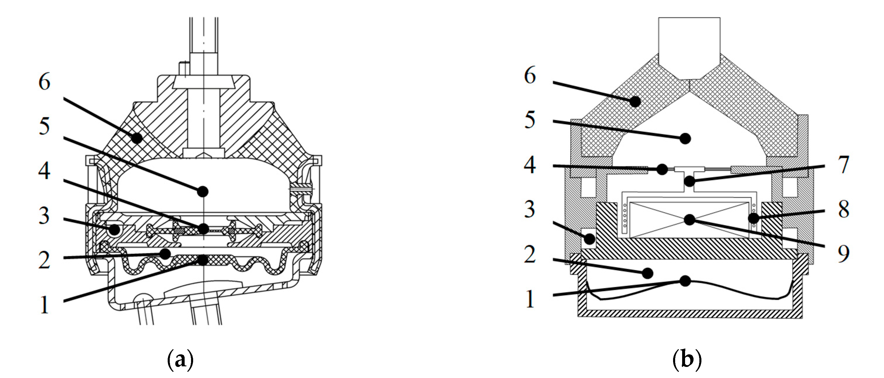
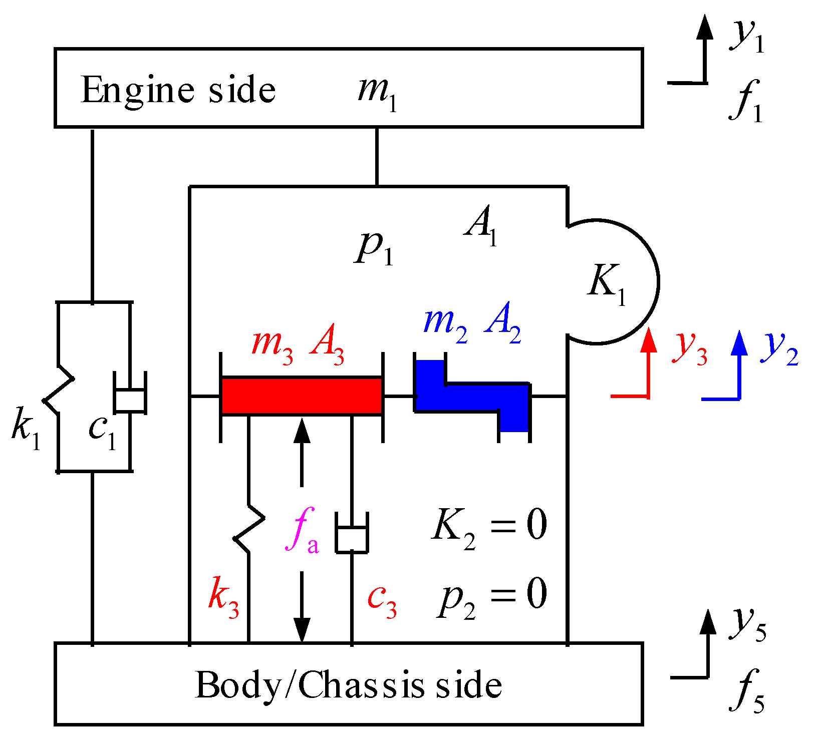
2. Mechanical Model of Active Hydraulic Mount (AHM)

Figure 1 shows the schematic diagram of (a) a passive hydraulic mount with inertia track and decoupler membrane (PHM-IT-DM) and (b) an AHM-IT-DM-OCA. The upper end is connected to engine, and the lower end is connected to body or chassis. In AHM-IT-DM-OCA, the coil skeleton is rigidly connected to the skeleton of the decoupler membrane to serve as an actuator mover. Alternating current (AC) power is applied to the coil. Then, the coil oscillates up and down under the alternating ampere force, which is induced in a constant magnetic field of a permanent magnet. The ampere force is the active force to be controlled. The active force is transmitted to the vehicle body through a secondary path to have the force transmitted from the engine to the vehicle body through the primary path canceled. The active force received by the actuator mover acts on the decoupler and simultaneously changes the dynamics of the hydraulic mount. The working mechanism of AHM-IT-DM-OCA can be understood either from the perspective of the actuator actively reducing the force transmitted to the vehicle body or from the perspective of the actuator actively adjusting the dynamic characteristics of the hydraulic mount.

Referring to the hydraulic mount mechanical models [5,6,7,8,9], a unified lumped parameter mechanical model for AHM-IT-DM and PHM-IT-DM is built, as shown in Figure 2. The displacement of the engine side is y₁ and the corresponding reaction force, i.e., the force acting on the mount, is f₁. The displacement of circularly flowing fluid in a horizontal plane relative to the wall of the fluid channel is y₂, and the mover displacement is y₃ (i.e., the decoupler for PHM-IT-DM). The displacement of the chassis side is y₅, and the force transmitted to the chassis is f₅. The pressure fluctuations in the upper and lower fluid chambers relative to the static state are p₁ and p₂, respectively. The active force of the actuator is f_a. These are variables for the lumped parameter model.

The vertical dynamic stiffness in-phase of main rubber spring is denoted as k₁, the viscous damping is c₁, and the equivalent mass on engine side is m₁. The reciprocating motion of the main rubber spring squeezes out and pumps in the fluid for the upper fluid chamber. The equivalent pumping piston area is denoted as A₁. Define bulk stiffness as a ratio of pressure change to corresponding volume change of a fluid chamber, i.e., dp/dV, in units of GN/m⁵; denote the bulk stiffness of main rubber spring as K₁ and that of rubber bellow as K₂. Due to the wrinkled rubber bellow, K₂ is several orders of magnitude smaller than K₁. Thus, K₂ is set to zero, and the pressure fluctuation in the lower fluid chamber is ignored and set p₂ = 0 [5,7,8,9]. Denote the length of inertia track as l₂, the cross-sectional area as A₂, the wet perimeter of cross section as L₂, and the hydraulic diameter as d₂ = 4A₂/L₂. For laminar flow (Reynolds number Re < 2320) [10], the loss factor of fluid flowing along the inertia track is ${\xi }_{l_2}=64\mu l_2/(\rho \left|{\dot{y}}_2\right|d_2^2)$, and denote the local loss factor of flowing fluid at entrance and outlet as ${\xi }_{d_2}$. Denote the mass of decoupler/mover as m₃, the linear stiffness as k₃, and the viscous damping as c₃. Denote the equivalent piston area of the decoupler membrane as A₃ and the bulk stiffness equivalent to linear stiffness k₃ as K₃. The equivalency relationship is as follows:

$$A_3^2{K}_3=k_3$$

(2)

These are parameters for the lumped parameter model.

It should be noted that, for the active and passive hydraulic mounts shown in Figure 1, the basic structure is a hydraulic engine mount with inertia track and decoupler membrane, so the mechanical model can be unified. As to specific components, the model parameter values are different. Specifically, the mass m₃ in the mechanical model refers to the mass of the decoupler for a PHM-IT-DM in Figure 1a and refers to the mass of the actuator mover for an AHM-IT-DM-OCA in Figure 1b. The active force f_a is always zero for a PHM-IT-DM, while for an AHM-IT-DM-OCA, the f_a is related to the excitation current i(t) or voltage u(t). When the actuator is powered off, an AHM-IT-DM-OCA will degenerate to a PHM-IT-DM.

The dynamic characteristics for an AHM can be divided into active and passive dynamics. The so-called passive dynamics refer to FRFs with input being the engine-side displacement and outputs being the reaction force of the engine side and the force transmitted to the chassis side when the chassis side is fixed and the actuator is powered off. These are drive-point and cross-point dynamic characteristics, respectively. The cross-point dynamics are primary path transfer functions in the control of an AHM. The so-called active dynamics refer to FRFs with input being current or voltage applied to actuator and outputs being engine-side reaction force and the force transmitted to chassis side when the engine side and chassis side being fixed. The active dynamics from the excitation current or voltage to the force transmitted to the chassis side are secondary path transfer functions in the control of an AHM. The transfer functions of primary and secondary paths affect the performance, stability, and the operating bandwidth for an active control mount.

An AHM-IT-DM involves the resonance of two subsystems, namely the resonance of the fluid channel and the resonance of mover. Experimental studies have shown that the natural frequency f_n3 of a fluid-filled mover is typically above 200 Hz, which is far greater than the natural frequency f_n2 of the fluid channel (typically less than 20 Hz). Because the two natural frequencies are far apart and based on the desire to simplify the inertia and damping forces in different frequency bands based on mechanical vibrations theory, the frequency bands are divided into low-, mid-, and high-frequency bands, as shown in Figure 3. The frequency bands below the natural frequency f_n3 of the mover shall also be referred to as mid-low-frequency bands and the corresponding dynamics as the mid-low-frequency dynamics. The frequency bands above the natural frequency f_n2 of the fluid channel shall be referred to as mid-high-frequency bands and the corresponding dynamic characteristics as the mid-high-frequency dynamics.

3. Analysis and Experimental Validation of Passive Dynamics

In this section, a nonlinear mathematical model for mid-low-frequency bands is established for passive dynamics of AHM-IT-DM-OCA, and the FRFs in fluid-filled state with the electromagnetic actuator off are studied. The engine-side displacement y₁ is used as an excitation, while the engine-side reaction forces f₁ and the force transmitted to chassis side f₅ are used as outputs. These are the drive-point dynamic stiffness and cross-point dynamic stiffness of a mount.

3.1. Nonlinear Lumped Parameter Mathematical Model for Passive Dynamics

Based on the unified mechanical model as shown in Figure 2, set m₁ = 0, y₅ = 0, and f_a = 0 to obtain the following nonlinear mathematical model for passive dynamics [8,9]:

$$\{\begin{array}{l}\rho l_2{\ddot{y}}_2+\frac{1}{2}\rho \left({\xi }_{l_2}+{\xi }_{d_2}\right)\left|{\dot{y}}_2\right|{\dot{y}}_2=-p_1\\ m_3{\ddot{y}}_3+c_3{\dot{y}}_3+k_3{y}_3+A_3{p}_1=0\\ A_2{y}_2+A_3{y}_3=A_1{y}_1+p_1/K_1\\ f_1=c_1{\dot{y}}_1+k_1{y}_1-A_1{p}_1\\ f_5=c_1{\dot{y}}_1+k_1{y}_1+c_3{\dot{y}}_3+k_3{y}_3-\left(A_1-A_3\right)p_1\\ =f_1-m_3{\ddot{y}}_3\end{array}$$

(3)

The equations are, in order, the Bernoulli equation for fluid flowing in inertia track, differential equation for mover motion, and the fluid continuity equation and equilibrium equation for engine-side reaction forces f₁ and transmitted force to chassis side f₅, respectively. For the fluid flowing in the inertia track, a nonlinear Bernoulli equation is used to account for the loss factor of fluid flowing along the fluid channel and local loss at the entrance and outlet [10].

3.2. Analysis of Mid-Low-Frequency Passive Dynamics and the Amplitude Dependence and Fixed Points (f << f_n3)

As stated above, the natural frequency f_n2 of the inertia track is much smaller than f_n3 of the mover, that is, f_n2 << f_n3. Considering mechanical vibrations theory [11], for an excitation frequency f << f_n3 in mid-low-frequency bands, the decoupler displacement y₃ is essentially in-phase with excitation. The excitation force is mainly balanced by elastic restoring force. Under this condition, the inertia and damping forces of the decoupler [6,7,8,11] may be neglected. Simplification of Equation (3) leads to the following mathematical model:

$$\{\begin{array}{l}\rho l_2{\ddot{y}}_2+\frac{1}{2}\rho \left({\xi }_{l_2}+{\xi }_{d_2}\right)\left|{\dot{y}}_2\right|{\dot{y}}_2=-p_1\\ k_3{y}_3+A_3{p}_1=0\\ A_2{y}_2+A_3{y}_3=A_1{y}_1+p_1/K_1\\ f_1=c_1{\dot{y}}_1+k_1{y}_1-A_1{p}_1\\ f_5=c_1{\dot{y}}_1+k_1{y}_1+k_3{y}_3-\left(A_1-A_3\right)p_1=f_1\end{array}$$

(4)

where f₅ = f₁ indicates that, in mid-low-frequency bands, drive-point passive dynamics are the same as cross-point ones, so there is no need to treat them differently. Eliminating the intermediate variables p₁ and y₃, it can be rewritten as follows:

$$\{\begin{array}{l}{\ddot{y}}_2+\left(\frac{32\mu }{\rho d_2^2}+\frac{{\xi }_{d_2}}{2l_2}\left|{\dot{y}}_2\right|\right){\dot{y}}_2+\frac{A_2{K}_{\mathrm{u}1}}{\rho l_2}{y}_2=\frac{A_1{K}_{\mathrm{u}1}}{\rho l_2}{y}_1\\ f_5=f_1=c_1{\dot{y}}_1+k_1{y}_1+A_1^2{K}_{\mathrm{u}1}{y}_1-A_1{A}_2{K}_{\mathrm{u}1}{y}_2\end{array}$$

(5)

where K_u1 is bulk stiffness of upper fluid chamber surrounded by main rubber spring and decoupler membrane. It consists of K₁ and K₃ in-series [12], as follows:

$$\frac{1}{K_{\mathrm{u}1}}=\frac{1}{K_1}+\frac{1}{K_3}$$

(6)

The in-series relationship makes the total bulk stiffness smaller than the smaller one of two bulk stiffnesses, that is, K_u1 < min (K₁, K₃). Equation (5) also shows that the various DOFs in AHM-IT-DM are decoupled from each other.

The multiple-scales perturbation analysis of second-order nonlinear damped vibration system has shown that [13], in terms of first-order approximation, the natural frequency is not affected by damping. In this case, the natural frequency of inertia track is as follows:

$$f_{\mathrm{n}2}=\frac{1}{2\pi }\sqrt{\frac{A_2}{\rho l_2}{K}_{\mathrm{u}1}},{\omega }_{\mathrm{n}2}=2\pi f_{\mathrm{n}2}$$

(7)

Experiments and numerical simulations have shown that [5], under excitation of harmonic displacement y₁, the responses of upper chamber pressure p₁, inertia fluid displacement y₂, decoupler/mover displacement y₃, and force transmitted to the chassis f₅ are all simple harmonics with the same frequency. Therefore, the following expressions can be assumed for the excitation and response:

$$y_1=Y_1{e}^{j\omega t},y_2=Y_2{e}^{j(\omega t-{\phi }_2)},f_1=f_5=F_1{e}^{j\omega t}=F_5{e}^{j\omega t}$$

(8)

where Y₁ is excitation displacement amplitude, a positive real number; Y₂ is response amplitude of inertia fluid displacement, a positive real number, φ₂ is loss angle of y₂ with respect to y₁; F₁ and F₅ are drive-point and cross-point response force amplitudes, respectively, which are complex numbers.

For a steady-state harmonic motion, the second-order nonlinear damping ${\xi }_{d_2}/2l_2$ due to local loss factor ${\xi }_{d_2}$ may be equivalised to a viscous damping of $4{\xi }_{d_2}\omega Y_2/3\pi l_2$ according to the principle of equivalent energy [11]. Substituting it into the first formula in Equation (5), we obtain the following:

$${\ddot{y}}_2+\left(\frac{32\mu }{\rho d_2^2}+\frac{4{\xi }_{d_2}}{3\pi l_2}\omega Y_2\right){\dot{y}}_2+{\omega }_{\mathrm{n}2}^2{y}_2=\frac{A_1{K}_{\mathrm{u}1}}{\rho l_2}{y}_1$$

(9)

Substituting Equation (8) into Equation (9) and the second formula of Equation (5), a set of algebraic equations are obtained. Solving them, the FRF of H₂ for fluid channel and the dynamic stiffness k^* for a hydraulic mount can be obtained:

$$H_2=\frac{Y_2}{Y_1}{e}^{-j{\phi }_2}=\frac{A_1}{A_2}\frac{1}{1-{\lambda }^2+j\left(C\lambda /{\omega }_{\mathrm{n}2}+D{Y}_2{\lambda }^2\right)}$$

(10)

$$k^{*}=\frac{F_5}{Y_1}=\frac{F_1}{Y_1}=k_1+A_1^2{K}_{\mathrm{u}1}+j\omega c_1-A_1^2{K}_{\mathrm{u}1}\frac{1}{1-{\lambda }^2+j\left(C\lambda /{\omega }_{\mathrm{n}2}+D{Y}_2{\lambda }^2\right)}$$

(11)

where $C=32\mu /\rho d_2^2$, $D=4{\xi }_{d_2}/3\pi l_2$, $\lambda ={\lambda }_2=\omega /{\omega }_{\mathrm{n}2}=f/f_{\mathrm{n}2}$.

Equation (10) shows the FRF, H₂, contains response amplitude Y₂ of inertia fluid, an unknown variable. Y₂ and H₂ may be calculated using a search method. For a given excitation amplitude Y₁, H₂ is calculated while Y₂ gradually increases from 0. When $\left|H_2\right|Y_1=Y_2$, Y₂ is the response amplitude of inertia fluid. Then, H₂ and k^* can be determined. Numerical simulations have shown the searched solutions have good properties, and each excitation amplitude has a unique response [5].

Equation (11) shows the mid-low-frequency passive dynamics are dependent on the response Y₂, which is uniquely determined by the excitation Y₁. Therefore, the mid-low-frequency passive dynamics of AHM-IT-DM are not only frequency-variant, but also amplitude-variant, i.e., there are different frequency-variant dynamic characteristics curves for different excitation amplitudes. The fundamental cause for amplitude-variant dynamics lies in the amplitude-dependent damping caused by local loss at the entrance and outlet. The amplitude-variant dynamic characteristics is a prerequisite for the existence of fixed points. In other words, for a lumped parameter model that only considers linear damping of the fluid, the dynamic characteristics are independent of the excitation amplitude, and it is impossible to express amplitude-variant dynamics. Thus, the linear model for AHM-IT-DM could not reveal the phenomenon concerning fixed points.

Based on Equation (11), the passive dynamics in mid-low-frequency bands can be analyzed, and a fixed point will be shown in passive dynamics. The following three situations are discussed:

(1) Low-frequency band when $\lambda \to 0$ (f << f_n2):

$$\begin{array}{l}{k}_0^{*}=k_1+j\omega c_1=k_0^{\prime }+j{k}_0^{″}\\ k_0^{\prime }=k_1,k_0^{″}=\omega c_1\end{array}$$

(12)

where $k_0^{*}$, $k_0^{\prime }$, and $k_0^{″}$ are dynamic stiffness, dynamic stiffness in-phase, and dynamic stiffness out-of-phase when $\lambda \to 0$, respectively. This result shows that, when the excitation frequency approaches to zero, the dynamics are that of the main rubber spring.

(2) Mid-frequency band when $\lambda \to \infty$ (f_n2 << f << f_n3):

$$\begin{array}{l}{k}_{\infty }^{*}=k_1+A_1^2{K}_{\mathrm{u}1}+j\omega c_1=k_{\infty }^{\prime }+j{k}_{\infty }^{″}\\ k_{\infty }^{\prime }=k_1+A_1^2{K}_{\mathrm{u}1}=k_{\infty ,1}^{\prime },k_{\infty }^{″}=\omega c_1\end{array}$$

(13)

where $k_{\infty }^{*}$, $k_{\infty }^{\prime }$, and $k_{\infty }^{″}$ are dynamic stiffness, dynamic stiffness in-phase, and dynamic stiffness out-of-phase when $\lambda \to \infty$, respectively. The result shows, when the fluid channel becomes almost turned off due to increasing fluid resistance with frequency, the passive dynamic stiffness in-phase in the mid-frequency band becomes constant, $k_{\infty ,1}^{\prime }=k_1+A_1^2{K}_{\mathrm{u}1}$, an identical horizontal segment in amplitude-dependent dynamic stiffness in-phase.

(3) Resonance frequency band when $\lambda \to 1$ ($f\to f_{\mathrm{n}2}$):

$$H_{2,1}=\frac{Y_2}{Y_1}{e}^{-j{\phi }_2}=-j\frac{A_1}{A_2}\frac{1}{C/{\omega }_{\mathrm{n}2}+D{Y}_2}$$

(14)

$$k_1^{*}=k_1+A_1^2{K}_{\mathrm{u}1}+j{\omega }_{\mathrm{n}2}{c}_1+j{A}_1^2{K}_{\mathrm{u}1}\frac{1}{C/{\omega }_{\mathrm{n}2}+D{Y}_2}$$

(15)

Note that Y₁ and Y₂ in Equation (14) are always positive, so H_2,1 is a pure imaginary number, and the imaginary part is negative. The loss angle is therefore ${\phi }_2=\pi /2$, indicating that the inertia fluid has a phase resonance when $\lambda =1$. By equating the real and imaginary parts on both sides, the following can be obtained:

$${\omega }_{\mathrm{n}2}D{Y}_2^2+C{Y}_2-{\omega }_{\mathrm{n}2}E{Y}_1=0$$

(16)

where $E=A_1/A_2$. Solving Equation (16) while keeping Y₂ positive, Y₂ is obtained:

$$Y_2=\frac{-C+\sqrt{C^2+4{\omega }_{\mathrm{n}2}^{2}DE{Y}_1}}{2{\omega }_{\mathrm{n}2}D}$$

(17)

Substituting Y₂ back into Equation (15), the dynamics can be obtained:

$$\begin{array}{l}{k}_1^{*}=k_1+A_1^2{K}_{\mathrm{u}1}+j{\omega }_{\mathrm{n}2}\left(c_1+\frac{2A_1^2{K}_{\mathrm{u}1}}{C+\sqrt{C^2+4{\omega }_{\mathrm{n}2}^{2}DE{Y}_1}}\right)=k_1^{\prime }+j{k}_1^{″}\\ k_1^{\prime }=k_1+A_1^2{K}_{\mathrm{u}1}=k_{\infty ,1}^{\prime },k_1^{″}={\omega }_{\mathrm{n}2}\left(c_1+\frac{2A_1^2{K}_{\mathrm{u}1}}{C+\sqrt{C^2+4{\omega }_{\mathrm{n}2}^{2}DE{Y}_1}}\right)\end{array}$$

(18)

where $k_1^{*}$, $k_1^{\prime }$, and $k_1^{″}$ are dynamic stiffness, dynamic stiffness in-phase, and dynamic stiffness out-of-phase when $f\to f_{\mathrm{n}2}$, respectively. Noted that equation (11) reveals the amplitude dependence of mid-low-frequency dynamics. However, Equation (18) shows that, when $\lambda =1$, the dynamic stiffness in-phase $k_1^{\prime }$ is a constant and independent of excitation amplitude Y₁. That is, under different amplitude excitations, the family of frequency-variant curves of dynamic stiffness in-phase all pass through the point where the frequency is f_n2 and the dynamic stiffness in-phase is $k_1^{\prime }=k_1+A_1^2{K}_{\mathrm{u}1}$. This is the fixed point, referred to as R, on passive dynamic stiffness in-phase.

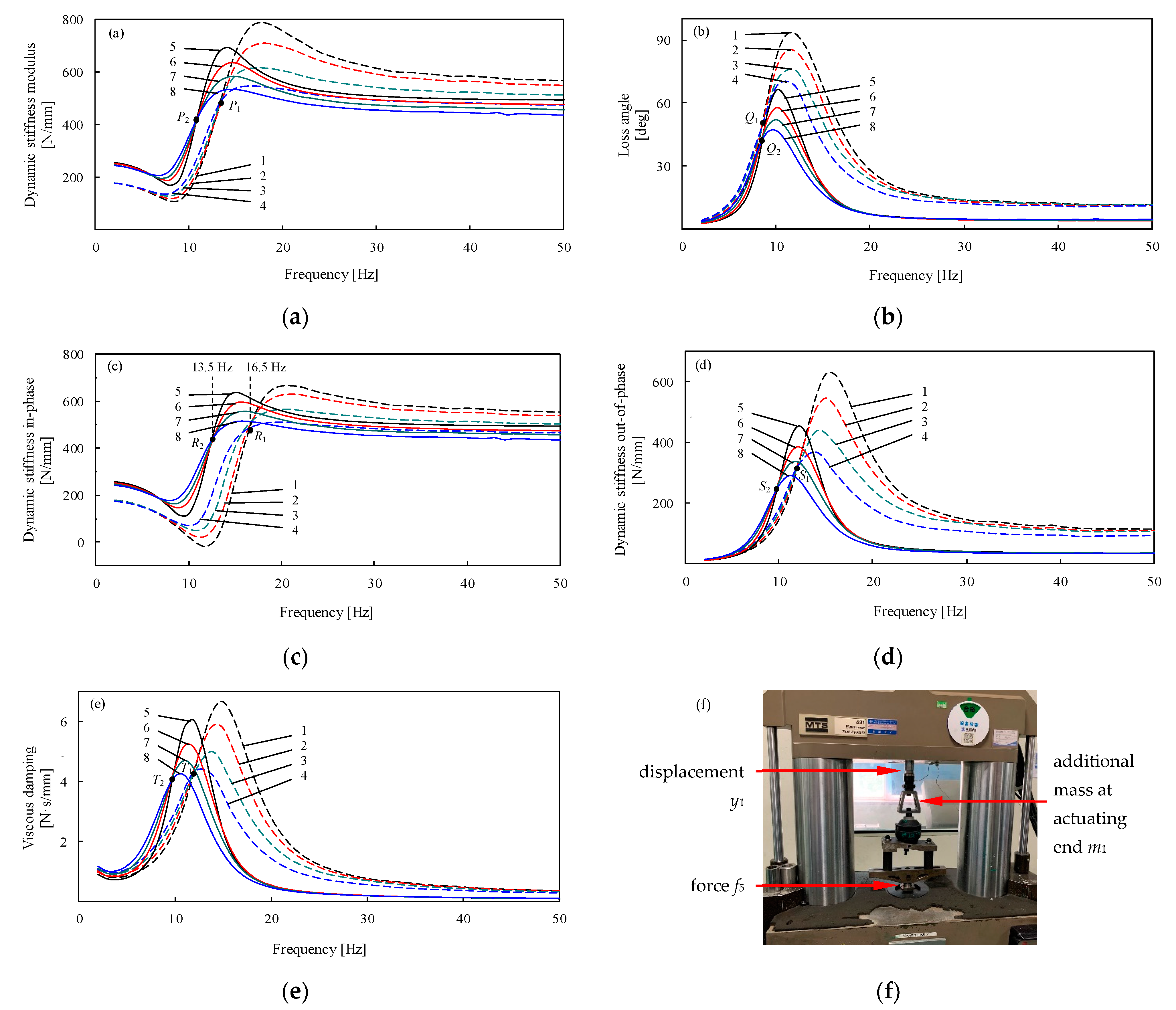
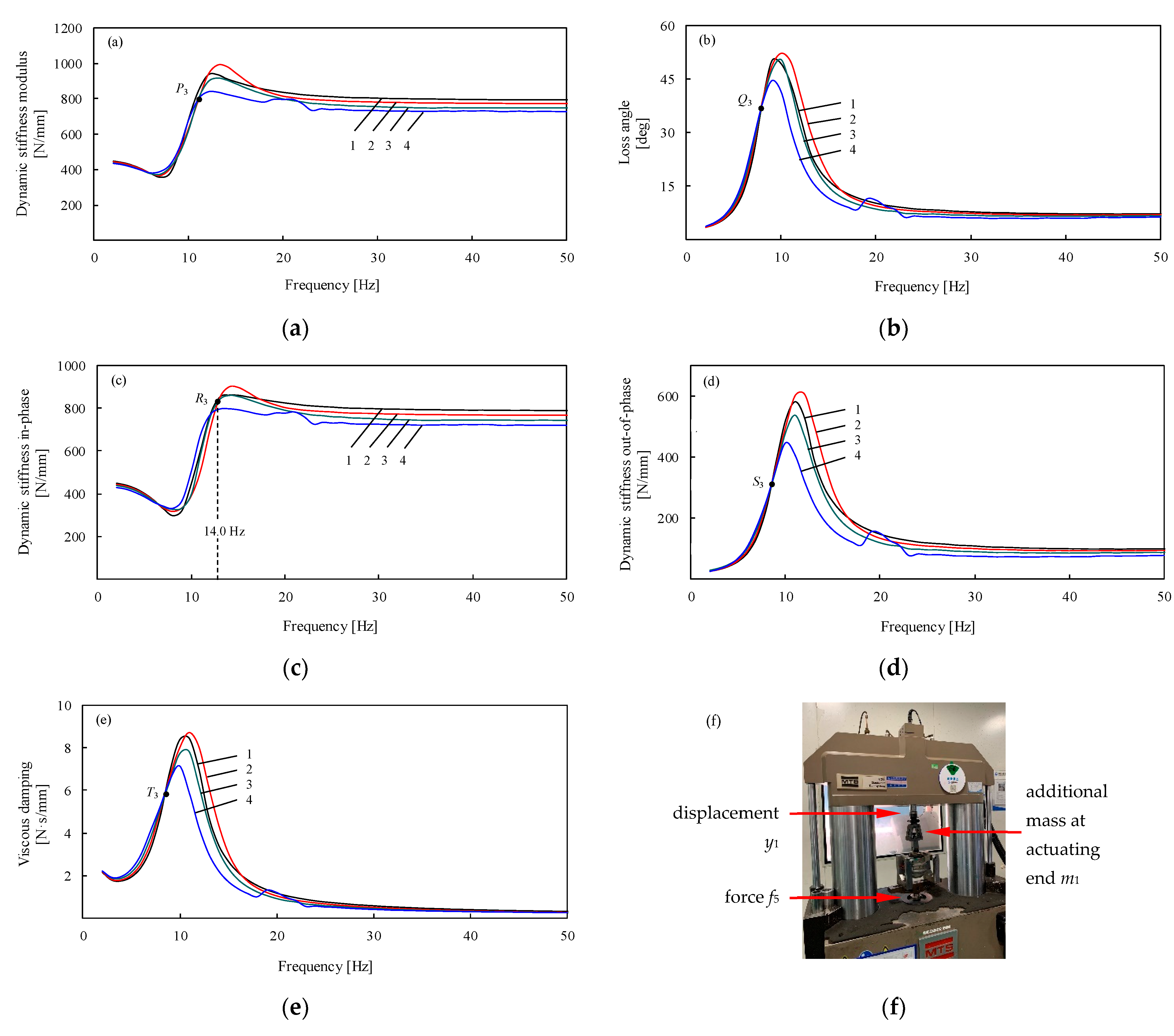
3.3. Experimental Validation of Amplitude Dependence and Fixed Point for Mid-Low-Frequency Passive Dynamics

The analysis shows that the distinct feature of the passive dynamics of AHM-IT-DM-OCAs is that a fixed point appears in mid-low-frequency bands due to amplitude dependence. To verify the amplitude dependence and fixed point, the following experiments are designed and carried out.

Two types of hydraulic mount, as shown in Figure 1, are tested. Figure 1a is PHM-IT-DM and Figure 1b is AHM-IT-DM-OCA, which degenerates to a PHM-IT-DM when the actuator is turned off. Their passive dynamics are used in verification of the features above. The tested results and associated experimental setups are shown in Figure 4 and Figure 5. As shown in Figure 4f and Figure 5f, the displacement y₁ and the transmitted force f₅ are tracked by the professional sensors of MTS Elastomer Test System.

Figure 4a–e show the experimental mid-low-frequency dynamics and fixed points of a PHM-IT-DM shown in Figure 1a. When excitation amplitude Y₁ is 0.4, 0.6, 0.8, and 1.0 mm (curves 5–8, respectively), the dynamics, i.e., the dynamic stiffness k, loss angle $\phi$, dynamic stiffness in-phase k′, dynamic stiffness out-of-phase k”, and viscous damping c, exhibit their fixed points P₂, Q₂, R₂, S₂, and T₂, respectively. The fixed points R₂ and the amplitude dependence in mid-low-frequency dynamics are clearly demonstrated as theoretically predicted in the analysis above. Curves 1–4 are the dynamics of a first-generation hydraulic mount, i.e., a PHM-IT, and the corresponding fixed points P₁, Q₁, R₁, S₁, and T₁, have been reported in [5]. It is noted that, due to differences in the construction and rubber materials between the previously tested PHM-IT and newly tested PHM-IT-DM, the parameter values are different, as are the fixed points.

Figure 5a–e show the experimental mid-low-frequency passive dynamics and fixed points of an AHM-IT-DM-OCA shown in Figure 1b. When the excitation amplitude Y₁ is 0.4, 0.6, 0.8, and 1.0 mm (curves 1–4, respectively), the passive dynamics also exhibit fixed points P₃, Q₃, R₃, S₃, and T₃, respectively, and amplitude dependence, as predicted in the analysis above.

Note that, in five different dynamics curves, as shown in Figure 4 and Figure 5, there always exists a peak in each curve, which is the resonance peak induced by fluid channel resonance.

Experimental studies have shown that there exists a single fixed point on each of the five dynamics curves in mid-low-frequency bands. Equation (18) just gives the theoretical solution of the fixed point, R, in dynamic stiffness in-phase. The solutions of the other four fixed points involve a challenging mathematical problem, i.e., solvable in terms of radicals of fifth order and higher algebraic equations. Abel rigorously proved that general algebraic equations higher than fourth order could not have general-form radical solutions, named the Abel–Ruffini theorem [14,15]. To determine whether the solutions of the other four fixed points belong to special equations with solutions in terms of radicals, it is necessary to study their solvability criteria based on the group theory, and this remains a topic for further investigation.

4. Analysis and Experimental Validation of Active Dynamics

In this section, the FRFs of a fluid-filled AHM-IT-DM-OCA with both the engine side and chassis side fixed and with the electromagnetic actuator operating are studied. The current i serves as an input excitation, and the reaction force f₁ and the force transmitted f₅ to the chassis side are outputs.

4.1. Nonlinear Lumped Parameter Zodel for Active Dynamics

Based on the AHM-IT-DM mechanical model in Figure 2, setting y₁ = 0 and y₅ = 0, the relationship between the actuator active force and excitation current is considered. With the oscillating coil as actuator, the following relationship exists:

$$f_{\mathrm{a}}\left(t\right)=Bli\left(t\right)=k_{\mathrm{M}}i\left(t\right)$$

(19)

where B is magnetic induction intensity, l is length of coil, and k_M is the voice coil constant, or so-called electromechanical coupling coefficient. The nonlinear mathematical model for active dynamics of AHM-IT-DM-OCAs is as follows:

$$\{\begin{array}{l}\rho l_2{\ddot{y}}_2+\frac{1}{2}\rho \left({\xi }_{l_2}+{\xi }_{d_2}\right)\left|{\dot{y}}_2\right|{\dot{y}}_2=-p_1\\ m_3{\ddot{y}}_3+c_3{\dot{y}}_3+k_3{y}_3+A_3{p}_1=f_{\mathrm{a}}\\ A_2{y}_2+A_3{y}_3=p_1/K_1\\ f_{\mathrm{a}}\left(t\right)=Bli\left(t\right)=k_{\mathrm{M}}i\left(t\right)\\ f_1=-A_1{p}_1\\ f_5=c_3{\dot{y}}_3+k_3{y}_3-\left(A_1-A_3\right)p_1-f_{\mathrm{a}}=f_1-m_3{\ddot{y}}_3\end{array}$$

(20)

4.2. Analysis of Mid-Low-Frequency Active Dynamics and the Amplitude Dependence and Fixed Points (f << f_n3)

Using the same simplification as in passive dynamics (Section 3.2), we neglect the inertia and damping forces of the actuator mover in mid-low-frequency bands, f << f_n3. The following nonlinear mathematical model is obtained:

$$\{\begin{array}{l}\rho l_2{\ddot{y}}_2+\frac{1}{2}\rho \left({\xi }_{l_2}+{\xi }_{d_2}\right)\left|{\dot{y}}_2\right|{\dot{y}}_2=-p_1\\ k_3{y}_3+A_3{p}_1=f_{\mathrm{a}}\\ A_2{y}_2+A_3{y}_3=p_1/K_1\\ f_{\mathrm{a}}\left(t\right)=Bli\left(t\right)=k_{\mathrm{M}}i\left(t\right)\\ f_1=-A_1{p}_1\\ f_5=k_3{y}_3-\left(A_1-A_3\right)p_1-f_{\mathrm{a}}=f_1\end{array}$$

(21)

After erasing the intermediate variables p₁ and y₃ and converting the second-order nonlinear fluid damping in a steady-state harmonic motion into an equivalent viscous damping, we have:

$$\{\begin{array}{l}{\ddot{y}}_2+\left(\frac{32\mu }{\rho d_2^2}+\frac{4{\xi }_{d_2}}{3\pi l_2}\omega Y_2\right){\dot{y}}_2+{\omega }_{n2}^2{y}_2=-\frac{K_{\mathrm{u}1}}{\rho l_2{A}_3{K}_3}{k}_{\mathrm{M}}i\\ f_5=f_1=-A_1{A}_2{K}_{\mathrm{u}1}{y}_2-\frac{A_1{K}_{\mathrm{u}1}}{A_3{K}_3}{k}_{\mathrm{M}}i\end{array}$$

(22)

where $i=I{e}^{j\omega t}$, and y₂, f₁, and f₅ are the same as in Equation (8). The first expression shows that the active and passive dynamics in mid-low-frequency bands shared the same fluid channel resonance frequency shown in Equation (7). In the second expression, f₅ = f₁, which means, in mid-low-frequency bands, the FRFs are from current to engine side, and those to the chassis side have the same active dynamics.

From Equation (22), we have the following FRFs for y₂ and f₅, respectively:

$$H_{2\mathrm{a}}=\frac{Y_2}{I}{e}^{-j{\phi }_2}=-\frac{k_{\mathrm{M}}}{A_2{A}_3{K}_3}\cdot \frac{1}{1-{\lambda }^2+j\left(C\lambda /{\omega }_{\mathrm{n}2}+D{Y}_2{\lambda }^2\right)}$$

(23)

$$-\frac{F_5}{I}=-\frac{F_1}{I}=\frac{A_1{K}_{\mathrm{u}1}}{A_3{K}_3}{k}_{\mathrm{M}}-\frac{A_1{K}_{\mathrm{u}1}}{A_3{K}_3}{k}_{\mathrm{M}}\cdot \frac{1}{1-{\lambda }^2+j\left(C\lambda /{\omega }_{\mathrm{n}2}+D{Y}_2{\lambda }^2\right)}$$

(24)

where C, D, and λ are the same as those in Equations (10) and (11). Equations (23) and (24) show that the mid-low-frequency active dynamics F₁/I and F₅/I are also frequency- and amplitude-dependent. If the amplitude I of excitation current is different, the response amplitude Y₂ will also be different. Then, the FRF curves are different. The amplitude dependence of the active dynamics may also imply the existence of a fixed point. We discuss the following three cases.

(1) Low-frequency band when $\lambda \to 0$ (f << f_n2):

$$-{\frac{F_5}{I}|}_{\lambda \to 0}=-{\frac{F_1}{I}|}_{\lambda \to 0}=0$$

(25)

(2) Mid-frequency band when $\lambda \to \infty$ (f_n2 << f << f_n3):

$$-{\frac{F_5}{I}|}_{\lambda \to \infty }=-{\frac{F_1}{I}|}_{\lambda \to \infty }=\frac{A_1{K}_{\mathrm{u}1}}{A_3{K}_3}{k}_{\mathrm{M}}=F_{i,\infty ,4}$$

(26)

This result means the following. First, f₅ and f_a have opposite directions in the mid-frequency band, or f₅ lags f_a by a phase angle of π, and the two are synchronously reversed. Second, the active FRFs of the mid-frequency band have only a real part, while the imaginary part is zero, which indicates the amplitude-frequency characteristics are equal to the real-frequency characteristics. Third, the active dynamics in the mid-frequency band tend to a constant, F_i,∞,4, an identical horizontal segment in the curves.

(3) Resonance frequency band where $\lambda \to 1$ ($f\to f_{\mathrm{n}2}$):

Using the same analysis method as in Section 3.2, we obtain the following:

$${-\frac{F_5}{I}|}_{\lambda =1}={-\frac{F_1}{I}|}_{\lambda =1}=\frac{A_1{K}_{\mathrm{u}1}}{A_3{K}_3}{k}_{\mathrm{M}}+j\frac{A_1{K}_{\mathrm{u}1}}{A_3{K}_3}{k}_{\mathrm{M}}\cdot \frac{2{\omega }_{\mathrm{n}2}}{C+\sqrt{C^2+4{\omega }_{\mathrm{n}2}^{2}D{E}_{\mathrm{a}}I}}$$

(27)

where $E_{\mathrm{a}}=k_{\mathrm{M}}/A_2{A}_3{K}_3$. This result shows, when λ = 1, i.e., the excitation frequency is equal to the fluid channel resonance frequency, the imaginary part still exhibits amplitude dependence, but the real part is a constant, which is independent of excitation amplitude. This means that, under different excitation amplitudes, the real-frequency characteristic curve family all pass through the point where the frequency is f_n2 and the real part is $A_1{K}_{\mathrm{u}1}{k}_{\mathrm{M}}/A_3{K}_3$, which is another fixed point on active real-frequency characteristics.

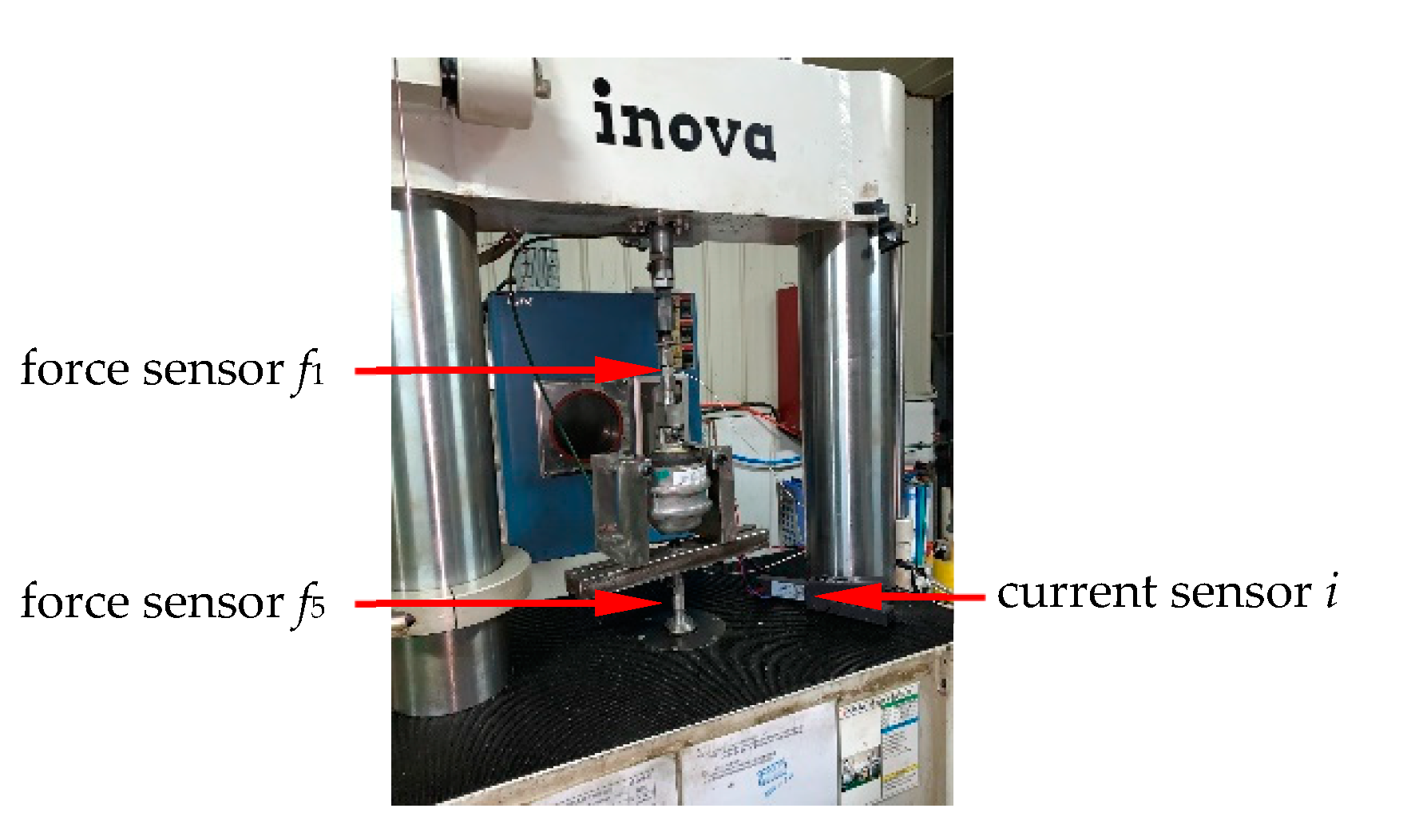
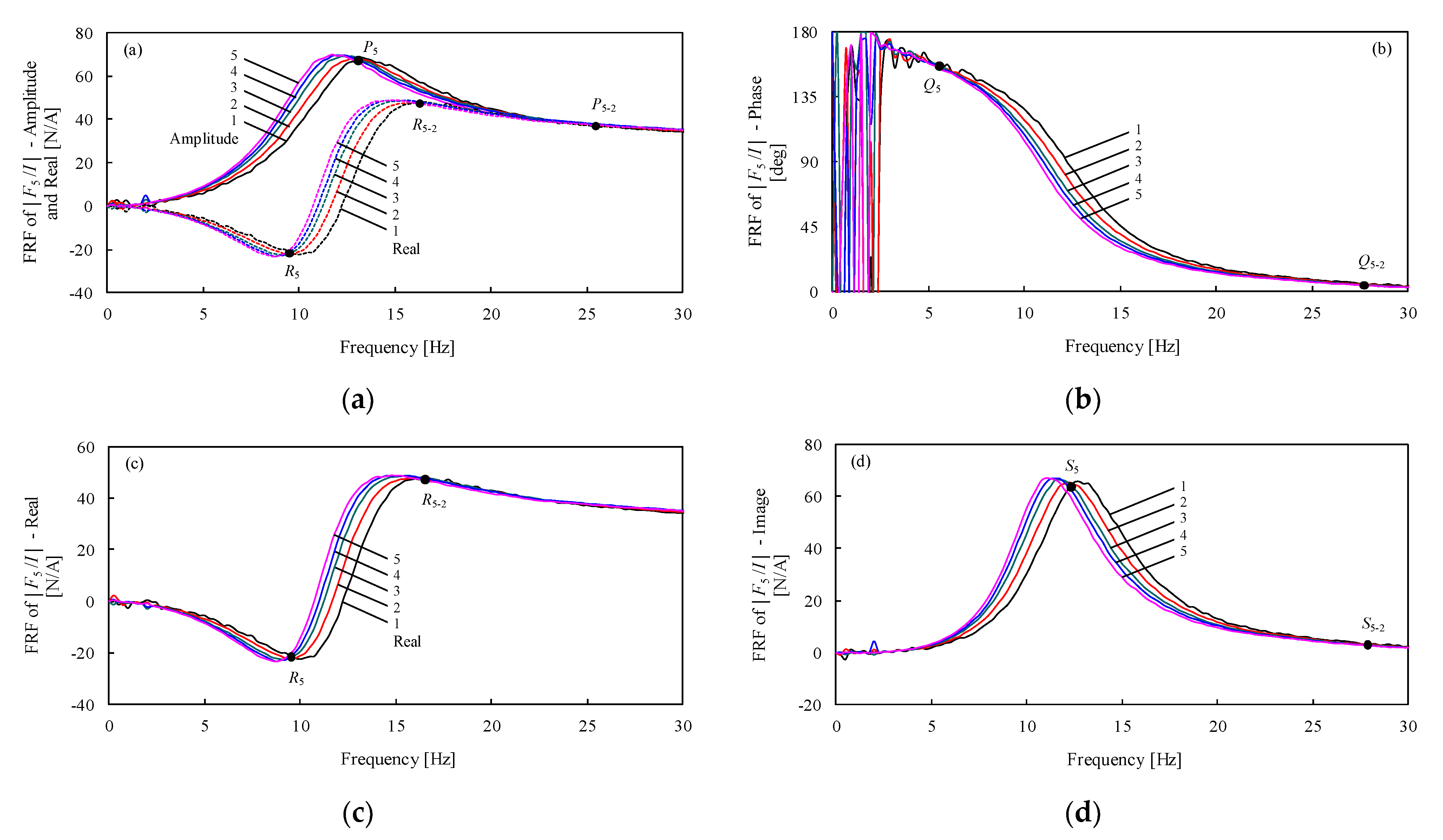
4.3. Experimental Validation of Amplitude Dependence and Fixed Point for Mid-Low-Frequency Active Dynamics

The analysis shows that the distinct features of active dynamics of AHM-IT-DM-OCAs are amplitude dependence and a fixed point in mid-low-frequency bands.

Figure 6 shows the test rig for active dynamics of an AHM-IT-DM-OCA. The upper and lower ends of the mount are fixed, and the actuator is excited with a burst random current i. The forces f₁ and f₅ at upper and lower ends are tracked by two force sensors of PCB 208C02 and the current is tracked by a current clamp of CHAUVIN ARNOUX E3N. The FRF curves of f₁ and f₅ with current i as input are obtained, as shown in Figure 7.

Figure 7 shows the tested active dynamics in mid-low-frequency bands, which clearly reflect the amplitude dependence and fixed points. Figure 7a also shows that the mid-band amplitude–frequency characteristics and their real part tend to be the same constant, i.e., the curves converge to an identical horizontal segment. The experimental phenomena, such as amplitude dependence, resonance peak, and horizontal segment, agree well with theoretical predictions in mid-frequency band. However, Figure 7 also shows the paired fixed points on each characteristic curve of amplitude, phase, and real and imaginary parts, such as P₅-P_5-2, Q₅-Q_5-2, R₅-R_5-2, and S₅-S_5-2, respectively. This is the first time that the paired fixed points have been demonstrated in experimental results. The analytical results regarding passive dynamics of AHM-IT-DM-OCA agree well with experiment, while the active dynamics also agree with the experiment, except the fixed point. The fundamental difference in active and passive dynamics is that the electromagnetic actuator is powered on or powered off. The mechanism for paired fixed points in active dynamics should be investigated in the future, considering the actuator structure and dynamic characteristics of electromagnetic induction.

5. Conclusions

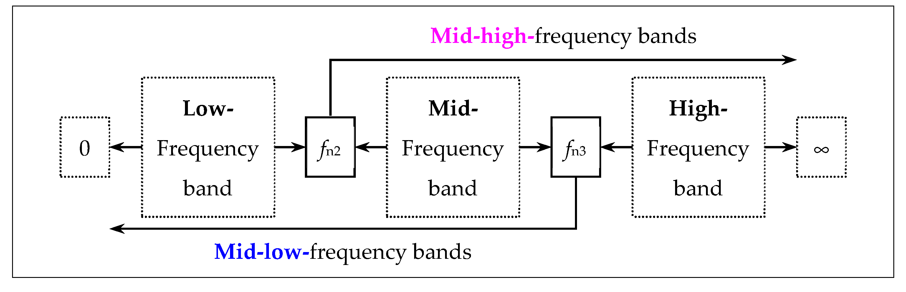
• A unified lumped parameter mechanical model with two DOFs is established for PHM-IT-DMs and AHM-IT-DMs. Considering that the fluid channel resonance frequency is far less than the resonance frequency of the decoupler/mover, the active and passive dynamics may be divided into mid-low-frequency dynamics and mid-high-frequency dynamics. In mid-low-frequency bands, the inertia and damping forces of decoupler/mover may be neglected, and a 1-DOF nonlinear lumped parameter mathematical model can be obtained.
• The 1-DOF nonlinear lumped parameter mathematical model for mid-low-frequency bands exhibits several distinct features in active and passive dynamics, such as amplitude dependence, fixed point, resonance peak, and horizontal segment.
• The fundamental reason for amplitude-dependent dynamics is the amplitude dependence of local loss at the entrance and outlet. Amplitude-dependent dynamics represent a precondition for the existence of a fixed point.
• Since the inertia of the decoupler/mover may be neglected in mid-low-frequency bands, the drive point and cross point dynamics are identical.
• A single fixed point in passive dynamics for an AHM-IT-DM-OCA is revealed in the analysis and experiment. In the meantime, a pair of fixed points in active dynamics is newly revealed in the experiment. This paired appearance of fixed points is a new issue, and its mechanism should be investigated considering the dynamic characteristics of electromagnetic induction.

References

1. Ormondroyd, J.; Den Hartog, J.P. The theory of the dynamic vibration absorber. ASME J. Appl. Mech 1928, 50, 9–22. [Google Scholar]
2. Hahnkamm, E. The damping of the foundation vibrations at varying excitation frequency. Master Arch. 1932, 4, 192–201. [Google Scholar]
3. Brock, J.E. A note on the damped vibration absorber. Trans. Am. Soc. Mech. Eng. 1946, 68, 284. [Google Scholar]
4. Den Hartog, J.P. Mechanical Vibrations, 4th ed.; McGraw-Hill: New York, NY, USA, 1956. [Google Scholar]
5. Fan, R.-L.; Lu, Z.-H. Fixed points on the nonlinear dynamic properties of hydraulic engine mounts and parameter identification method: Experiment and theory. J. Sound Vib. 2007, 305, 703–727. [Google Scholar] [CrossRef]
6. He, S.; Singh, R. Estimation of amplitude and frequency dependent parameters of hydraulic engine mount given limited dynamic stiffness measurements. Noise Control Eng. J. 2005, 53, 271–285. [Google Scholar] [CrossRef] [Green Version]
7. Hausberg, F.; Christian, S.; Peter, P.; Manfred, P.; Simon, H.; Markus, R. Experimental and analytical study of secondary path variations in active engine mounts. J. Sound Vib. 2015, 340, 22–38. [Google Scholar] [CrossRef]
8. Fan, R.-L.; Dou, Y.-F.; Yao, F.-H.; Qi, S.-Q.; Han, C. Experimental and analytical study of secondary path transfer function in active hydraulic mount with solenoid actuator. Actuators 2021, 10, 150. [Google Scholar] [CrossRef]
9. Fan, R.-L.; Wang, P.; Han, C.; Wei, L.-J.; Liu, Z.-J.; Yuan, P.-J. Summarisation, simulation and comparison of nine control algorithms for an active control mount with an oscillating coil actuator. Algorithms 2021, 14, 256. [Google Scholar] [CrossRef]
10. Gao, Z.-Q.; Wang, B.-R. Fluid Mechanics; Science Press: Beijing, China, 2017. [Google Scholar]
11. Zhang, Y.-M. Mechanical Vibrations; Tsinghua University Press: Beijing, China, 2019. [Google Scholar]
12. Fan, R.-L.; Fei, Z.-N.; Zhou, B.-Y.; Gong, H.-B.; Song, P.-J. Two-step dynamics of a semiactive hydraulic engine mount with four-chamber and three-fluid-channel. J. Sound Vib. 2020, 480, 115403. [Google Scholar] [CrossRef]
13. Wen, B.-C. Engineering Nonlinear Vibrations; Science Press: Beijing, China, 2007. [Google Scholar]
14. Khovanskii, A. Topological Galois Theory. Solvability and Unsolvability of Equations in Finite Terms; Springer: Berlin/Heidelberg, Germany, 2014. [Google Scholar]
15. Esterov, A. Galois theory for general systems of polynomial equations. Compos. Math. 2019, 155, 229–245. [Google Scholar] [CrossRef] [Green Version]
Figure 1. Configuration schematics for PHM-IT-DM and AHM-IT-DM-OCA. (a) PHM-IT-DM; (b) AHM-IT-DM-OCA. Key: 1. rubber bellow; 2. lower chamber; 3. inertia track; 4. decoupler membrane; 5. upper chamber; 6. main rubber spring; 7. decoupler/actuator mover; 8. coil; 9. permanent magnet.
Actuators 10 00225 g001
Figure 2. Unified lumped parameter mechanical model for AHM-IT-DMs and PHM-IT-DMs.
Actuators 10 00225 g002
Figure 3. Low-, mid-, and high-frequency bands for AHM-IT-DM-OCA.
Actuators 10 00225 g003
Figure 4. Experimental validation of the passive dynamic properties in mid-low-frequency bands and the fixed points Pi, Qi, Ri, Si, and Ti (i = 1,2) of a PHM-IT and a PHM-IT-DM. (a) Dynamic stiffness modulus; (b) loss angle; (c) dynamic stiffness in-phase; (d) dynamic stiffness out-of-phase; (e) viscous damping; (f) test rig. Key: The numbers 1–4 correspond to the PHM-IT under excitation amplitudes of Y1 = 0.4, 0.6, 0.8, and 1.0 mm, respectively [5]; the numbers 5–8 correspond to the PHM-IT-DM under excitations of Y1 = 0.4, 0.6, 0.8, and 1.0 mm, respectively.
Actuators 10 00225 g004
Figure 5. Experimental validation of the passive dynamic properties in mid-low-frequency bands and the fixed points P3, Q3, R3, S3, and T3 of an AHM-IT-DM-OCA. (a) Dynamic stiffness modulus; (b) loss angle; (c) dynamic stiffness in-phase; (d) dynamic stiffness out-of-phase; (e) viscous damping; (f) test rig. Key: The numbers 1–4 correspond to excitation amplitudes of Y1 = 0.4, 0.6, 0.8, and 1.0 mm, respectively.
Actuators 10 00225 g005
Figure 6. Experimental setup for active dynamics of an AHM-IT-DM-OCA in fluid-filled state.
Actuators 10 00225 g006
Figure 7. Experimental validation for the active dynamic properties in mid-low-frequency bands and the paired fixed points P5P5-2, Q5Q5-2, R5R5-2, and S5S5-2 of an AHM-IT-DM-OCA in fluid-filled state. (a) Amplitude and real part of the FRFs; (b) phase of the FRFs; (c) real part of the FRFs; (d) imaginary part of the FRFs. Key: The numbers 1–5 correspond to excitation current amplitudes of I = 1, 3, 5, 7 and 9 A, respectively.
Actuators 10 00225 g007
Publisher’s Note: MDPI stays neutral with regard to jurisdictional claims in published maps and institutional affiliations.