Boundary-Adapted Numerical Modeling of Flow in a Hydrostatic Leadscrew

Abstract

A new method is presented to model and predict the flow fields of the hydrostatic leadscrews with greater accuracy. It is different from those available methods, in which various bearings are assumed to be equivalent to the screw-nut pair within a pitch by various means. In this new method, a helical coordinate system adapting to the boundaries of the flow fields is constructed, which makes the screw-nut meshing clearance calculated more accurate. Based on the finite difference method (FDM), the meshing clearance is discretized into a number of flow fields, which are created by numerous couples of parallel-plate elements moving relatively along the helicoid. The numerical model is solved in MATLAB, and the analyses about the pressure fields demonstrate its favorable performances in reflecting the actual flow fields. Furthermore, the simulation results are compared with the experimental values, confirming the feasibility of the proposed method.

1. Introduction

The hydrostatic leadscrews are widely used for precision machining, and increasingly high demands are placed on them. The numerical studies of the systems can circumvent many obstacles inherent in the experiments, and thus reduce the test costs, which is of great significance for the developments of the prototype machines.

Conventionally, scholars have simplified the hydrostatic and aerostatic leadscrews as a series connection of various thrust bearings using diverse approaches. Through the axial projection of the intermeshing helicoids, the helical gap flow fields were simplified as multiple annular flow fields by Wertwijn and Klarich [1], Matataro and Akira [2,3], Satomi and Yamamoto [4,5], Zhao and Satomi [6], Shen [7], Luo and Zhao [8], Zhong [9], and Xin [10]. Somewhat differently, El-Sayed and Khataan [11,12,13], Zhang [14,15] and Ohishi [16] expanded the intermeshing helicoids within a pitch into a couple of annular-sector plates according to some approximate rules, to obtain the annular-sector flow fields. Besides, the aerostatic leadscrews were replaced by multiple taper bearings in the studies of Lu and Yu et al. [17].

A drawback of the approximation methods of axial projection and tapered bearing substitution is that the influences of torsion and the lead angle are ignored, thus the actual conditions of flow fields are poorly reflected.

With the lead angle and thread angle both covered, the sector approximation method is superior to the others. In the method, there is a one-to-one mapping from the finite-difference elements of the helicoid to the those of the annular sector. Furthermore, there are some approximate rules to be followed between the sums of the elements of the helicoid and those of the sector.

Theoretically, the areas of two bounded surfaces with different shapes may be different even if the sides of them are of equal length, respectively, such as a bounded plane and a bounded curved surface, with the same length on each boundary. In [11], the restrictions were placed only on the lengths of the flow-field boundaries, not the areas, which may make such parameters as the lead angle, thread angle, arc length, torsion, and curvature of each grid element approximated to varying degrees. If such variations occur, then the calculated flow-field pressures would deviate from the actual values. The reason for this is that the pressure values are strongly related to the areas and shapes of the loading surfaces, although the directions of the speed and the pressure at each node remain consistent before and after approximation. As is well known, the denser the meshes, the smaller the deviations caused by the aforesaid approximations, but the according computing costs will increase significantly. Furthermore, there may be a divergence problem of solutions with the increase of the number of grid elements. Lastly, the grid elements may change to adapt to the different discretization methods of the fluid equations and geometric parameters of the system.

Available studies on the flow-field modeling of the hydrostatic and aerostatic leadscrews are quite few. Although the sector approximation method would be superior to the others theoretically, the solutions based on the method were not strictly verified, and the flow fields were not reflected well. In view of the shortcomings of the current methods, a new modeling method, in which a follow-up coordinate system adapting to the boundaries of the flow fields is constructed along the pitch diameter helix of the nut, is proposed in this research, to provide a more convincing prediction of the flow fields.

In this research, the method is implemented and discussed by MATLAB. Compared with the common flow-field simulations in the CFD professional software, the simulations in MATLAB are realized by converting all the information into MATLAB codes, without three-dimensional geometric models of the flow fields.

2. Materials and Methods

2.1. Construction of Helical Coordinate System Adapting to the Boundaries of the Flow Fields

A screw-driven hydrostatic leadscrew with a six-turn-thread nut was chosen as the research object to describe the new modeling method, and four oil chambers were assumed to be evenly spaced on each of the four turns of threads in the middle of the nut.

The leadscrew was assumed to be oriented vertically for the convenience of description. The flow fields on the upper side of the nut were named the upper flow fields, and those on the other side were named the lower flow fields. Besides, the research was carried out under the following assumptions: (1) the pressure gradient along the film thickness direction is 0; (2) the outer boundary pressure is 0; (3) the velocity gradient in the helical direction can be ignored, compared with the thickness direction; (4) the volume force and inertia force can be neglected, compared with the viscous force; (5) the research involves only laminar motion of an incompressible Newtonian fluid; (6) the boundary velocities satisfy the no-slip condition; and (7) the normal section of fit clearance is assumed as rectangular, with a trapezoidal thread discussed in this research.

The Lagrange method was adopted to describe the flow fields in this research [18]. The upper flow fields were taken for example. As shown in Figure 1a,b, “$\mathit{O}{\mathit{\xi }}_1{\mathit{\xi }}_2{\mathit{\xi }}_3$” is a global coordinate system (“$\mathit{O}\mathit{r}\mathit{\theta }{\mathit{\xi }}_3$” is the corresponding cylindrical coordinate system), and “${\mathit{O}}_1\mathit{X}\mathit{Y}\mathit{Z}$” is a local inertial frame fixed on the nut. The ${\mathit{O}}_1\mathit{Z}$-axis coincided with the $\mathit{O}{\mathit{\xi }}_3$-axis, and the ${\mathit{O}}_1\mathit{X}$-axis intersected the upper helicoid of the nut at point $e$ on the pitch diameter helix. With counterclockwise rotations defined as positive, the screw rotation angle $\theta$ was calculated, starting from the position of the ${\mathit{O}}_1\mathit{X}$-axis at the initial time. For a right-hand-thread leadscrew, the nut moves downwards along the axial direction when the screw is turned counterclockwise. Point $e$ in Figure 1a,b,d is the starting point of the helical coordinate system, point $E$ in Figure 1b is any point on the $s$-axis, point $F$ in Figure 1b, e is a point whose distance from point $E$ in the ${\mathit{y}}^{\prime }$ direction is $h$, and $h$ is the clearance thickness of the gap flow fields. The normal section “$\mathit{n}$-$\mathit{n}$” of the screw is shown in Figure 1c, the section of the gap fields at the initial time is shown in Figure 1d, and the relations among velocity components of point $F$ are shown in Figure 1e.

As shown in Figure 1b,d, a helical coordinate system “$\mathit{sy}$”, composed of the $\mathit{s}$-axis and a follow-up coordinate system “$\mathit{oxy}$”, was constructed on the upper helicoid of the nut [19,20]. The $\mathit{s}$-axis gone from point $e$ along the pitch diameter helix of the helicoid, and “$\mathit{oxy}$” changed along the $\mathit{s}$-axis (tangent vector $\mathit{t}$) to adapt to the normal and binormal vectors ($\mathit{n}$ and $\mathit{b}$) of the Frenet frame of pitch diameter helix.

The origin $o$ of the follow-up coordinate system could be any point on the pitch diameter helix. ${\mathit{R}}_{\mathrm{f}}$ was employed to locate point $o$ in “${\mathit{O}}_1\mathit{XYZ}$”, and the position of the point in “$\mathit{O}{\mathit{\xi }}_1{\mathit{\xi }}_2{\mathit{\xi }}_3$” could be expressed as Equation (1):

$${\mathit{R}}_o={\mathit{R}}_{O_1}+{\mathit{R}}_{\mathrm{f}}$$

(1)

The position of point O₁ in “$\mathit{O}{\mathit{\xi }}_1{\mathit{\xi }}_2{\mathit{\xi }}_3$” was described by ${\mathit{R}}_{O_1}$, whose relationship with the axial displacement of the nut $Z_{\mathrm{nut}}$ was:

$${\mathit{R}}_{O_1}=-Z_{\mathrm{nut}}\mathit{k}$$

(2)

$\mathit{i}$, $\mathit{j}$ and $\mathit{k}$ are the unit vectors in the ${\mathit{\xi }}_1$, ${\mathit{\xi }}_2$ and ${\mathit{\xi }}_3$ direction, respectively.

An arbitrary point in the fields could be located in “$\mathit{O}{\mathit{\xi }}_1{\mathit{\xi }}_2{\mathit{\xi }}_3$” through Equation (3):

$$\begin{array}{l}{\mathit{R}}_{\mathrm{A}}={\mathit{R}}_{O_1}+{\mathit{R}}_{\mathrm{f}}+x\mathit{n}+y\mathit{b}\\ ={\mathit{R}}_{O_1}+{\mathit{R}}_{{}_{\mathrm{hA}}}\end{array}$$

(3)

${\mathit{R}}_{\mathrm{hA}}$ is the position of the arbitrary point in “$\mathit{sxy}$” or “${\mathit{O}}_1\mathit{XYZ}$”. “$\mathit{O}{\mathit{\xi }}_1{\mathit{\xi }}_2{\mathit{\xi }}_3$” and “${\mathit{O}}_1\mathit{XYZ}$” were coincident at the coordinate origin at the initial moment, that was to say, ${\mathit{R}}_{O_1}=0$ at the moment.

The Frenet frame of the $\mathit{s}$-axis in “${\mathit{O}}_1\mathit{XZ}$” could be solved based on Equations (4)–(6), to evaluate the orthogonality of the helical coordinate system.

$$\mathit{t}=\frac{\partial {\mathit{R}}_{\mathrm{hA}}}{\partial s}=(-\frac{r_{\mathrm{m}}}{\sqrt{r_{\mathrm{m}}{}^2+{(\frac{P}{2\pi })}^2}}\sin \theta ,\frac{r_{\mathrm{m}}}{\sqrt{r_{\mathrm{m}}{}^2+{(\frac{P}{2\pi })}^2}}\cos \theta ,\frac{\frac{P}{2\pi }}{\sqrt{r_{\mathrm{m}}{}^2+{(\frac{P}{2\pi })}^2}})$$

(4)

$$\mathit{n}=\frac{1}{\kappa }\frac{\mathrm{d}\mathit{t}}{\mathrm{d}s}=(-\cos \theta ,-sin\theta ,0)$$

(5)

$$\mathit{b}=\mathit{t}\times \mathit{n}=(\frac{\frac{P}{2\pi }}{\sqrt{r_{\mathrm{m}}{}^2+{(\frac{P}{2\pi })}^2}}\sin \theta ,-\frac{\frac{P}{2\pi }}{\sqrt{r_{\mathrm{m}}{}^2+{(\frac{P}{2\pi })}^2}}\cos \theta ,\frac{r_{\mathrm{m}}}{\sqrt{r_{\mathrm{m}}{}^2+{(\frac{P}{2\pi })}^2}})$$

(6)

The arc length was calculated:

$$\mathrm{d}{\mathit{R}}_{\mathrm{hA}}\mathrm{d}{\mathit{R}}_{\mathrm{hA}}=\left({\left(1-\kappa x\right)}^2+{\left(\tau y\right)}^2+{\left(\tau x\right)}^2\right){\left(\mathrm{d}s\right)}^2+{\left(\mathrm{d}x\right)}^2+{\left(\mathrm{d}y\right)}^2+2\tau x\mathrm{d}s\mathrm{d}y-2\tau y\mathrm{d}x\mathrm{d}s$$

(7)

Here, $P$, $\kappa$, $\tau$, and $r_{\mathrm{m}}$ are the pitch, curvature, torsion, and pitch radius of the helix along the $\mathit{s}$-axis, respectively. $r_{\mathrm{m}}$ was supposed to be equal to the pitch radius of the gap fields.

The helical coordinate system “$\mathit{s}\mathit{x}\mathit{y}$” was considered to be non-orthogonal, according to the judgment rule [21].

Shown in Figure 1b,d, according to the methods for rotating the Frenet frame in [21,22], each follow-up coordinate system “$\mathit{o}\mathit{x}\mathit{y}$” was rotated by $\phi$ ($\phi$ is half of the thread angle of the normal section at the position with a radius of $r_{\mathrm{m}}$ in Figure 1. Modeling diagram based on the helical coordinate system. (a) Schematic diagram; (b) modeling of fluid domain; (c) “-” of the screw; (d) initial section; (e) velocity relations.c) around the $\mathit{s}$-axis to obtain a new follow-up coordinate system “$\mathit{o}{\mathit{x}}^{\prime }{\mathit{y}}^{\prime }$”. In the corresponding new helical coordinate system “$\mathit{s}{\mathit{x}}^{\prime }{\mathit{y}}^{\prime }$”, the normal and binormal vectors (${\mathit{n}}^{\prime }$ and ${\mathit{b}}^{\prime }$) of the new Frenet frame were aligned with the corresponding flow field boundaries, respectively.

The normal and binormal vectors before and after rotation satisfied the relationships:

$${\mathit{n}}^{\prime }=\mathit{n}\cos \phi -\mathit{b}\sin \phi$$

(8)

$${\mathit{b}}^{\prime }=\mathit{n}\sin \phi +\mathit{b}\cos \phi$$

(9)

The position of any selected point in “$\mathit{s}{\mathit{x}}^{\prime }{\mathit{y}}^{\prime }$” after rotation could be described as:

$${\mathit{R}}_{\mathrm{hA}}={\mathit{R}}_{\mathrm{f}}+{\mathrm{x}}^{\prime }{\mathit{n}}^{\prime }+{\mathrm{y}}^{\prime }{\mathit{b}}^{\prime }$$

(10)

Similar to Equation (7), the arc length was calculated:

$$\begin{array}{l}\mathrm{d}{\mathit{R}}_{\mathrm{hA}}\mathrm{d}{\mathit{R}}_{\mathrm{hA}}=({(1-\kappa x^{\prime }\cos \phi -\kappa y^{\prime }\sin \phi )}^2+(x^{\prime }(\frac{\mathrm{d}(\cos \phi )}{\mathrm{d}s}+\tau \sin \phi )+y^{\prime }{(\frac{\mathrm{d}(\sin \phi )}{\mathrm{d}s}-\tau \cos \phi ))}^2\\ +(x^{\prime }(\tau \cos \phi -\frac{\mathrm{d}(\sin \phi )}{\mathrm{d}s})+y^{\prime }(\tau \sin \phi +\frac{\mathrm{d}(\cos \phi )}{\mathrm{d}s}))){\left(\mathrm{d}s\right)}^2+({\cos }^2\phi +{\sin }^2\phi ){(\mathrm{d}{x}^{\prime })}^2+({\cos }^2\phi +{\sin }^2\phi ){(\mathrm{d}{y}^{\prime })}^2\\ +2y^{\prime }(\frac{\partial \phi }{\partial s}-\tau )\mathrm{d}s\mathrm{d}{x}^{\prime }+2x^{\prime }(\tau -\frac{\partial \phi }{\partial s})\mathrm{d}s\mathrm{d}{y}^{\prime }\end{array}$$

(11)

It could be deduced from Equation (11) that the new helical coordinate system was not orthogonal until $\tau =\frac{\partial \phi }{\partial s}$, and then there was such a relation as follows:

$$\frac{\partial {\mathit{R}}_{\mathrm{hA}}}{\partial s}=\left(1-\kappa x^{\prime }\cos \phi -\kappa y^{\prime }\sin \phi \right)\mathit{t}$$

(12)

In light of the above analyses, the helical coordinate system was deduced to be non-orthogonal with a constant $\phi$.

As mentioned above, the Lagrangian description was employed during the process. The relative motion of the fluid particle in “${\mathit{O}}_1\mathit{XYZ}$” was analyzed firstly for convenience, and then the absolute motion in “$\mathit{O}{\mathit{\xi }}_1{\mathit{\xi }}_2{\mathit{\xi }}_3$” was solved based on the theory of relative motion (refer to the relations shown in Figure 1e).

A mapping between “$\mathit{s}{\mathit{x}}^{\prime }{\mathit{y}}^{\prime }$” and “$\mathit{O}{\mathit{\xi }}_1{\mathit{\xi }}_2{\mathit{\xi }}_3$”was obtained through Equation (13):

$$\begin{array}{l}{\mathit{R}}_{\mathrm{A}}={\mathit{R}}_{O_1}+{\mathit{R}}_{\mathrm{f}}+x^{\prime }{\mathit{n}}^{\prime }+y^{\prime }{\mathit{b}}^{\prime }\\ =(r_{\mathrm{m}}\cos \theta -(x^{\prime }\cos \phi +y^{\prime }\sin \phi )\cos \theta +(y^{\prime }\cos \phi -x^{\prime }\sin \phi )\frac{\frac{P}{2\pi }}{\sqrt{r_{\mathrm{m}}{}^2+{(\frac{P}{2\pi })}^2}}\sin \theta )\mathit{i}\\ +(r_{\mathrm{m}}\sin \theta -(x^{\prime }\cos \phi +y^{\prime }\sin \phi )\sin \theta -(y^{\prime }\cos \phi -x^{\prime }\sin \phi )\frac{\frac{P}{2\pi }}{\sqrt{r_{\mathrm{m}}{}^2+{(\frac{P}{2\pi })}^2}}\cos \theta )\mathit{j}\\ +(\frac{P}{2\pi }\theta -Z_{\mathrm{nut}}+(y^{\prime }\cos \phi -x^{\prime }\sin \phi )\frac{r_{\mathrm{m}}}{\sqrt{r_{\mathrm{m}}{}^2+{(\frac{P}{2\pi })}^2}})\mathit{k}\\ ={\xi }_1\mathit{i}+{\xi }_2\mathit{j}+{\xi }_3\mathit{k}\end{array}$$

(13)

2.2. Derivation of Reynolds Equation in Helical Coordinate System

In the following analyses, the group of symbols “$s,x,y$” was utilized to replace “$s,x^{\prime },y^{\prime }$” after rotation, and to locate the flow-field particles in the new helical coordinate system, for ease of description. As mentioned in Section 2.1, the motions of fluid particles relative to the nut are analyzed in this section.

According to the assumptions in (1)–(7) in Section 2.1, the Navier–Stokes equation could be simplified as follows [21,22,23]:

$$\{\begin{array}{c}\frac{1}{M}\frac{\partial p}{\partial s}=\eta \frac{{\partial }^2\omega }{\partial y^2}\\ \frac{\partial p}{\partial x}=\eta \frac{{\partial }^{2}u}{\partial y^2}\end{array}$$

(14)

The continuity equation could be reduced as follows:

$$\frac{\partial (Mu)}{\partial x}+\frac{\partial (Mv)}{\partial y}+(y\frac{\partial \omega }{\partial x}-x\frac{\partial \omega }{\partial y})\tau +\frac{\partial \omega }{\partial s}=0$$

(15)

where $M=1-\kappa x\cos \phi -\kappa y\sin \phi$, and the velocities of any fluid particle in the $\mathit{x}$, $\mathit{y}$, and $\mathit{s}$ direction were indicated by such vectors as “$\mathit{u},\mathit{v},\mathit{w}$”, respectively.

$M=1-\kappa x\cos \phi$ was assumed, as the order of magnitude in the $\mathit{y}$ direction was much smaller than that in other directions. Then, the first formula in Equation (14) was developed into:

$$\frac{1}{1-\kappa x\cos \phi }\frac{\partial p}{\partial s}=\eta \frac{{\partial }^2\omega }{\partial y^2}$$

(16)

It could be deduced that $\frac{\partial p}{\partial y}=0$ from the assumption in (1) in Section 2.1.

The upper flow fields were taken for example. The fluid particle, which was stationary relative to the nut, was assumed to have a $y$-coordinate of 0 (“${\mathit{u}}_1,{\mathit{v}}_1,{\mathit{w}}_1$”). There was no slip motion between the screw and the particle whose $y$-coordinate was $h$ (“${\mathit{u}}_2,{\mathit{v}}_2,{\mathit{w}}_2$”).

When Equation (16) was integrated twice with respect to $y$, $\omega$ was obtained:

$$\omega =\frac{1}{2\eta \left(1-\kappa x\cos \phi \right)}\frac{\partial p}{\partial s}\left(y^2-hy\right)+\frac{1}{h}\left({\omega }_2-{\omega }_1\right)y+{\omega }_1$$

(17)

where, for $x\in \forall$, $w(x)$ is true as long as $y=0$.

When the second formula in Equation (14) was integrated twice with respect to $x$, $u$ was given by:

$$u=\frac{1}{2\eta }\frac{\partial p}{\partial x}\left(y^2-yh\right)$$

(18)

The unit discharges in the $\mathit{s}$ and $\mathit{x}$ direction could be solved by:

$$q_s={\displaystyle {\int }_0^h\omega \mathrm{d}y}=-\frac{1}{12}\frac{h^3}{\left(1-\kappa x\cos \phi \right)\eta }\frac{\partial p}{\partial s}+\frac{1}{2}\left({\omega }_1+{\omega }_2\right)h$$

(19)

$$q_x={\displaystyle {\int }_0^{h}u\mathrm{d}y}=-\frac{1}{12\eta }\frac{\partial p}{\partial x}{h}^3$$

(20)

Equation (15) was developed into:

$$(-\kappa \cos \phi )u+(1-\kappa x\cos \phi )\frac{\partial u}{\partial x}+(1-\kappa x\cos \phi )\frac{\partial v}{\partial y}+(y\frac{\partial \omega }{\partial x}-x\frac{\partial \omega }{\partial y})\tau +\frac{\partial \omega }{\partial s}=0$$

(21)

Here, the term $y\frac{\partial \omega }{\partial x}$ could be ignored, because $\frac{\partial \omega }{\partial x}<<\frac{\partial \omega }{\partial y}$. When Equation (21) was integrated with respect to $y$, the simplified Reynolds equation [24,25] was obtained:

$$\begin{array}{l}\frac{\partial }{\partial x}((1-\kappa x\cos \phi )(-\frac{1}{12\eta }{h}^3)\frac{\partial p}{\partial x})+\frac{\partial }{\partial s}(-\frac{h^3}{12(1-\kappa x\cos \phi )\eta }\frac{\partial p}{\partial s})\\ =-(1-\kappa x\cos \phi )({\nu }_2-{\nu }_1)+\tau x({\omega }_2-{\omega }_1)+\frac{1}{2}\frac{\partial h}{\partial s}({\omega }_1+{\omega }_2)-\frac{1}{2}h\frac{\partial ({\omega }_1+{\omega }_2)}{\partial s}\end{array}$$

(22)

2.3. Boundary Conditions of the Helical Flow Fields

In the light of the kinematics principle of particle and the theory of moving coordinate system [26,27], the relations among the velocity components of the fluid particle, which makes no slip motion relative to the screw, are shown in Figure 1e. Then, a set of relations could be deduced from ${\mathit{v}}_x+{\mathit{v}}_y+{\mathit{v}}_s={\mathit{v}}_{\mathrm{r}}$:

$$\{\begin{array}{c}{v}_s=v_{\mathrm{r}}\cos \delta \\ \sqrt{{\left(v_y\right)}^2+{\left(v_x\right)}^2}=v_{\mathrm{r}}\sin \delta \end{array}$$

(23)

$$v_{\mathrm{r}}=\sqrt{{\stackrel{•}{Z}}_{\mathrm{nut}}{}^2+v_{\mathrm{screw}}{}^2}=\sqrt{{\stackrel{•}{Z}}_{\mathrm{nut}}{}^2+{(r\Omega )}^2}$$

(24)

Here, ${\mathit{v}}_{\mathrm{r}}$${\overrightarrow{v}}_r$ is the relative velocity of a fluid particle, ${\mathit{v}}_x$, ${\mathit{v}}_y$, and ${\mathit{v}}_s$ are the velocities of the particle in the $\mathit{x}$, $\mathit{y}$, and $\mathit{s}$ direction, respectively, $\delta$ is the angle between ${\mathit{v}}_{\mathrm{r}}$ and ${\mathit{v}}_s$, and ${\stackrel{•}{Z}}_{\mathrm{nut}}$ is the axial velocity of the nut. And then,

$$\delta \approx \left|{\lambda }_r-{\lambda }_{r_{\mathrm{m}}}\right|$$

(25)

$${\lambda }_r=\arctan (\frac{P}{2\pi r})$$

(26)

$${\stackrel{•}{Z}}_{\mathrm{nut}}=\frac{P}{2\pi }\Omega +\mathsf{\Delta }\stackrel{•}{Z}$$

(27)

$$\mathsf{\Delta }Z=\mathsf{\Delta }h\cos {\lambda }_{r_{\mathrm{m}}}\cos \phi$$

(28)

$$h=h_{\mathrm{n}0}+\mathsf{\Delta }h$$

(29)

where ${\lambda }_r$ is the lead angle of the helix at the position with a radius of $r$, $\Delta h$ is the transient variation of clearance thickness, $\Delta Z$ is the transient displacement from the equilibrium position of the nut caused by $\Delta h$, and $\Delta \stackrel{•}{Z}$ is the change rate of $\Delta Z$. Thus, $v_s$ could be defined by:

$$v_s=\sqrt{{(\frac{P\Omega }{2\pi }+\mathsf{\Delta }\stackrel{•}{Z})}^2+{(\Omega r)}^2}\cos ({\lambda }_r-{\lambda }_{r_{\mathrm{m}}})$$

(30)

When $v_x$ was ignored, $v_y\approx v_{\mathrm{r}}\sin \delta$.

Then, the boundary conditions of the flow fields are presented in

Table 1. Boundary conditions of the fields.

Upper Fields
Parameter	Value	Parameter	Value
$y_1$	0	$y_2$	$h$
$u_1$	0	$u_2$	0
$v_1$	0	$v_2$	$v_{\mathrm{r}}\sin \delta$
${\omega }_1$	0	${\omega }_2$	$v_{\mathrm{r}}\cos \delta$
Lower Fields
Parameter	Value	Parameter	Value
$y_1$	$-h$	$y_2$	0
$u_1$	0	$u_2$	0
$v_1$	$v_{\mathrm{r}}\sin \delta$	$v_2$	0
${\omega }_1$	$v_{\mathrm{r}}\cos \delta$	${\omega }_2$	0

2.4. Solution of Reynolds Equation Applicable to a Screw-Nut Pair

2.4.1. Discretization of Reynolds Equation

The following relations were supposed:

$$\Delta h=\Delta h_{\mathrm{s}}+\Delta h_{\mathrm{d}}$$

(31)

$$p=p_{\mathrm{s}}+p_{Z_{\mathrm{d}}}\mathsf{\Delta }{Z}_{\mathrm{d}}+p_{{\stackrel{•}{Z}}_{\mathrm{d}}}\mathsf{\Delta }{\stackrel{•}{Z}}_{\mathrm{d}}$$

(32)

Here, $\mathsf{\Delta }{h}_{\mathrm{s}}$ is the steady component of $\mathsf{\Delta }h$, $\mathsf{\Delta }{h}_{\mathrm{d}}$ is the disturbed component, $\mathsf{\Delta }{Z}_{\mathrm{d}}$ is the axial displacement perturbation caused by $\mathsf{\Delta }{h}_{\mathrm{d}}$, $\Delta {\stackrel{•}{Z}}_d$ is the change rate of $\mathsf{\Delta }{Z}_{\mathrm{d}}$, $p_{Z_{\mathrm{d}}}$ is the first-order pressure disturbance caused by $\mathsf{\Delta }{Z}_{\mathrm{d}}$, $p_{{\stackrel{•}{Z}}_{\mathrm{d}}}$ is the second-order pressure disturbance caused by $\mathsf{\Delta }{\stackrel{•}{Z}}_{\mathrm{d}}$ [28].

Through the definitions:

$x=h_{\mathrm{n}0}\overline{x}$, $y=h_{\mathrm{n}0}\overline{y}$, $s=h_{\mathrm{n}0}\overline{s}$, $\kappa =h_{\mathrm{n}0}\epsilon$, $g=h_{\mathrm{n}0}\tau$, $p=P_{\mathrm{s}}\overline{p}$, $h=h_{\mathrm{n}0}\overline{h}$, $\mathsf{\Delta }Z=h_{\mathrm{n}0}\overline{\mathsf{\Delta }Z}$, $\Omega =\frac{P_{\mathrm{s}}{h}_{\mathrm{n}0}{}^2}{\eta r_{\mathrm{m}}{}^2}\overline{\Omega }$, $\overline{A}=1-\epsilon \overline{x}\cos \phi$, $A{s}_1=\sqrt{{(\frac{P\overline{\Omega }}{2\pi h_{\mathrm{n}0}})}^2+{(\overline{r}\overline{\Omega })}^2}$, $A{s}_2=\sqrt{\frac{P\overline{\Omega }}{\pi h_{\mathrm{n}0}}}$, the dimensionless transient Reynolds equation of the upper flow fields was given by:

$$\begin{array}{l}\frac{1}{12}\epsilon \cos \phi {\overline{h}}_{\mathrm{s}}{}^3\frac{\partial {\overline{p}}_{\mathrm{s}}}{\partial \overline{x}}-\frac{1}{4}\overline{A}{\overline{h}}_{\mathrm{s}}{}^2\frac{\partial {\overline{h}}_{\mathrm{s}}}{\partial \overline{x}}\frac{\partial {\overline{p}}_{\mathrm{s}}}{\partial \overline{x}}-\frac{1}{12}\overline{A}{\overline{h}}_{\mathrm{s}}{}^3\frac{{\partial }^2{\overline{p}}_{\mathrm{s}}}{\partial {\overline{x}}^2}-\frac{1}{4}\frac{1}{\overline{A}}{\overline{h}}_{\mathrm{s}}{}^2\frac{\partial {\overline{h}}_{\mathrm{s}}}{\partial \overline{s}}\frac{\partial {\overline{p}}_{\mathrm{s}}}{\partial \overline{s}}-\frac{1}{12}\frac{1}{\overline{A}}{\overline{h}}_{\mathrm{s}}{}^3\frac{{\partial }^2{\overline{p}}_{\mathrm{s}}}{\partial {\overline{s}}^2}\\ +(\frac{1}{12}\epsilon \cos \phi (3{\overline{h}}_{\mathrm{s}}{}^2\frac{\partial {\overline{p}}_{\mathrm{s}}}{\partial \overline{x}}\frac{1}{\cos {\lambda }_{r_{\mathrm{m}}}\cos \phi }+{\overline{h}}_{\mathrm{s}}{}^3\frac{\partial {\overline{p}}_{Z_{\mathrm{d}}}}{\partial \overline{x}})-\frac{1}{12}\overline{A}(6{\overline{h}}_{\mathrm{s}}\frac{\partial {\overline{h}}_{\mathrm{s}}}{\partial \overline{x}}\frac{\partial {\overline{p}}_{\mathrm{s}}}{\partial \overline{x}}\frac{1}{\cos {\lambda }_{r_{\mathrm{m}}}\cos \phi }+3{\overline{h}}_{\mathrm{s}}{}^2\frac{{\partial }^2{\overline{p}}_{\mathrm{s}}}{\partial {\overline{x}}^2}\frac{1}{\cos {\lambda }_{r_{\mathrm{m}}}\cos \phi }\\ +3{\overline{h}}_{\mathrm{s}}{}^2\frac{\partial {\overline{h}}_{\mathrm{s}}}{\partial \overline{x}}\frac{\partial {\overline{p}}_{{\overline{Z}}_{\mathrm{d}}}}{\partial \overline{x}}+{\overline{h}}_{\mathrm{s}}{}^3\frac{{\partial }^2{\overline{p}}_{{\overline{Z}}_{\mathrm{d}}}}{\partial {\overline{x}}^2})-\frac{1}{12}\frac{1}{\overline{A}}(6{\overline{h}}_{\mathrm{s}}\frac{\partial {\overline{h}}_{\mathrm{s}}}{\partial \overline{s}}\frac{\partial {\overline{p}}_{\mathrm{s}}}{\partial \overline{s}}\frac{1}{\cos {\lambda }_{r_m}\cos \phi }+3{\overline{h}}_{\mathrm{s}}{}^2\frac{{\partial }^2{\overline{p}}_{\mathrm{s}}}{\partial {\overline{x}}^2}\frac{1}{\cos {\lambda }_{r_{\mathrm{m}}}\cos \phi }+3{\overline{h}}_{\mathrm{s}}{}^2\frac{\partial {\overline{h}}_{\mathrm{s}}}{\partial \overline{s}}\frac{\partial {\overline{p}}_{{\overline{Z}}_{\mathrm{d}}}}{\partial \overline{s}}\\ +{\overline{h}}_{\mathrm{s}}{}^3\frac{{\partial }^2{\overline{p}}_{{\overline{Z}}_{\mathrm{d}}}}{\partial {\overline{s}}^2}))\mathsf{\Delta }{\overline{Z}}_{\mathrm{d}}+(\frac{1}{12}\epsilon \cos \phi {\overline{h}}_{\mathrm{s}}{}^3\frac{\partial {\overline{p}}_{{\stackrel{•}{\overline{Z}}}_{\mathrm{d}}}}{\partial \overline{x}}-\frac{1}{12}\overline{A}(3{\overline{h}}_{\mathrm{s}}{}^2\frac{\partial {\overline{h}}_{\mathrm{s}}}{\partial \overline{x}}\frac{\partial {\overline{p}}_{{\stackrel{•}{\overline{Z}}}_{\mathrm{d}}}}{\partial \overline{x}}+{\overline{h}}_{\mathrm{s}}{}^3\frac{{\partial }^2{\overline{p}}_{{\stackrel{•}{\overline{Z}}}_{\mathrm{d}}}}{\partial {\overline{x}}^2})-\frac{1}{12}\frac{1}{\overline{A}}(3{\overline{h}}_{\mathrm{s}}{}^2\frac{\partial {\overline{h}}_{\mathrm{s}}}{\partial \overline{s}}\frac{\partial {\overline{p}}_{{\stackrel{•}{\overline{Z}}}_{\mathrm{d}}}}{\partial \overline{s}}+\\ {\overline{h}}_{\mathrm{s}}{}^3\frac{{\partial }^2{\overline{p}}_{{\stackrel{•}{\overline{Z}}}_{\mathrm{d}}}}{\partial {\overline{s}}^2}))\mathsf{\Delta }{\stackrel{•}{\overline{Z}}}_{\mathrm{d}}\\ =-\overline{A}\sin \delta A{s}_1+(g\overline{x}+\frac{1}{2}\frac{\partial {\overline{h}}_{\mathrm{s}}}{\partial \overline{s}})\cos \delta A{s}_1+(-\overline{A}\sin \delta A{s}_2+(g\overline{x}+\frac{1}{2}\frac{\partial {\overline{h}}_{\mathrm{s}}}{\partial \overline{s}})\cos \delta A{s}_2)\mathsf{\Delta }{\stackrel{•}{\overline{Z}}}_{\mathrm{d}}\end{array}$$

(33)

The five-point finite difference method (FDM) was employed to discretize the Reynolds equation in Equation (33), and the kth iterative pressure was given by:

$$\begin{array}{l}{p}^{\left(k\right)}\left(i,j\right)=\omega (\frac{1}{En(i,j)}(An(i,j)p^{\left(k-1\right)}(i+1,j)+Bn\left(i,j\right)p^{\left(k\right)}\left(i-1,j\right)+Cn\left(i,j\right)p^{\left(k\right)}\left(i,j+1\right)+Dn\left(i,j\right)p^{\left(k\right)}\left(i,j-1\right))\\ -Fn\left(i,j\right))+p^{\left(k-1\right)}\left(i,j\right)\end{array}$$

(34)

The steady state were taken as an example. The coefficients are given by:

$$An(i,j)=-\frac{\overline{A}(i,j)}{16}{\overline{h}}_{\mathrm{s}}{}^2(i,j)\frac{1}{{(\mathsf{\Delta }\overline{x})}^2}({\overline{h}}_{\mathrm{s}}(i+1,j)-{\overline{h}}_{\mathrm{s}}(i-1,j))-\frac{\overline{A}(i,j)}{12}{\overline{h}}_{\mathrm{s}}{}^3(i,j)\frac{1}{{(\mathsf{\Delta }\overline{x})}^2}+\frac{1}{24}\epsilon \cos \phi \frac{1}{\mathsf{\Delta }\overline{x}}{\overline{h}}_{\mathrm{s}}{}^3(i,j)$$

(35)

$$Bn(i,j)=\frac{\overline{A}(i,j)}{16}{\overline{h}}_{\mathrm{s}}{}^2(i,j)\frac{1}{{\left(\mathsf{\Delta }\overline{x}\right)}^2}\left({\overline{h}}_{\mathrm{s}}(i+1,j)-{\overline{h}}_{\mathrm{s}}(i-1,j)\right)-\frac{\overline{A}(i,j)}{12}{\overline{h}}_{\mathrm{s}}{}^3(i,j)\frac{1}{{\left(\mathsf{\Delta }\overline{x}\right)}^2}-\frac{1}{24}\epsilon \cos \phi \frac{1}{\mathsf{\Delta }\overline{x}}{\overline{h}}_{\mathrm{s}}{}^3(i,j)$$

(36)

$$Cn(i,j)=-\frac{1}{16\overline{A}(i,j)}{\overline{h}}_{\mathrm{s}}{}^2(i,j)\frac{1}{{\left(\mathsf{\Delta }\overline{s}\right)}^2}\left({\overline{h}}_{\mathrm{s}}(i,j+1)-{\overline{h}}_{\mathrm{s}}(i,j-1)\right)-\frac{1}{12\overline{A}(i,j)}{\overline{h}}_{\mathrm{s}}{}^3(i,j)\frac{1}{{\left(\mathsf{\Delta }\overline{s}\right)}^2}$$

(37)

$$Dn(i,j)=\frac{1}{16\overline{A}(i,j)}{\overline{h}}_{\mathrm{s}}{}^2(i,j)\frac{1}{{\left(\mathsf{\Delta }\overline{s}\right)}^2}\left({\overline{h}}_{\mathrm{s}}(i,j+1)-{\overline{h}}_{\mathrm{s}}(i,j-1)\right)-\frac{1}{12\overline{A}(i,j)}{\overline{h}}_{\mathrm{s}}{}^3(i,j)\frac{1}{{\left(\mathsf{\Delta }\overline{s}\right)}^2}$$

(38)

$$En(i,j)=-\frac{\overline{A}(i,j)}{6}{\overline{h}}_{\mathrm{s}}{}^3(i,j)\frac{1}{{\left(\mathsf{\Delta }\overline{x}\right)}^2}-\frac{1}{6\overline{A}(i,j)}{\overline{h}}_{\mathrm{s}}{}^3(i,j)\frac{1}{{\left(\mathsf{\Delta }\overline{s}\right)}^2}$$

(39)

$$Fn(i,j)=-\overline{A}(i,j)A{s}_1(i,j)\sin \left(\delta (i,j)\right)+\left(g\overline{x}(i,j)+\frac{1}{2}\frac{\partial {\overline{h}}_{\mathrm{s}}(i,j)}{\partial \overline{s}}\right)A{s}_1(i,j)\cos \left(\delta (i,j)\right)$$

(40)

where “$i$” and “$j$” are applicable to all internal nodes.

2.4.2. Solutions of Pressure and Flow

As shown in Figure 2, fluids were assumed to flow out of an oil chamber in four directions, and the distribution of oil chambers in one of the four turns of helical fields was obtained by means of an axial projection [29]. The chambers were counterclockwise named as “Chamber 1”, “Chamber 2”, “Chamber 3”, and “Chamber 4”.

$$Q_{\mathrm{out}}=Q_1+Q_2+Q_3+Q_4$$

(41)

Here, $Q_{\mathrm{out}}$ is the total flow of an oil chamber for a certain time.

Continuing from Section 2.4.1, the upper flow fields in the steady state were still taken for example. On the basis of Equations (19) and (20), the dimensionless discharges in each direction could be given as follows:

$${\overline{Q}}_1={\displaystyle \int (\frac{1}{12}(\frac{1}{\overline{A}}{\overline{h}}_{\mathrm{s}}{}^3\frac{\partial {\overline{p}}_{\mathrm{s}}}{\partial \overline{s}})-\frac{1}{2}({\overline{h}}_{\mathrm{s}}A{s}_1\cos \delta ))}\mathrm{d}\overline{x}$$

(42)

$${\overline{Q}}_2=-{\displaystyle \int (\frac{1}{12}(\frac{1}{\overline{A}}{\overline{h}}_{\mathrm{s}}{}^3\frac{\partial {\overline{p}}_{\mathrm{s}}}{\partial \overline{s}})-\frac{1}{2}({\overline{h}}_{\mathrm{s}}A{s}_1\cos \delta ))}\mathrm{d}\overline{x}$$

(43)

$${\overline{Q}}_3=\frac{1}{12}{\displaystyle \int ({\overline{h}}_{\mathrm{s}}{}^3\frac{\partial {\overline{p}}_{\mathrm{s}}}{\partial \overline{x}})}\mathrm{d}\overline{s}$$

(44)

$${\overline{Q}}_4=-\frac{1}{12}{\displaystyle \int ({\overline{h}}_{\mathrm{s}}{}^3\frac{\partial {\overline{p}}_{\mathrm{s}}}{\partial \overline{x}})}\mathrm{d}\overline{s}$$

(45)

$Q_{\mathrm{out}}$ could be solved by summing over Equations (42)–(45).

The capillary restrictor was taken as an example. The relationship between the chamber pressure and flow could be obtained according to the flow continuity through an oil chamber:

$$P_{\mathrm{r}}Csc=Csc-Q_{\mathrm{out}}$$

(46)

here, $Csc$ is the throttle coefficient. And the node pressures in the same oil chamber were considered to be equal.

Based on Equations (34)–(46), the node pressures of the upper fields in the steady state could be solved through the method of successive over-relaxation (SOR) [28,30,31,32].

2.5. Solution of Static and Dynamic Characteristic Parameters

Only the axial static and dynamic characteristics were studied in this research.

$$W={\displaystyle {\int }_{}^{}{\displaystyle {\int }_{}^{}\left(\left(p_{\mathrm{Bs}}-p_{\mathrm{Ts}}\right)\cos {\lambda }_{r_{\mathrm{m}}}\cos \phi +\eta \sin {\lambda }_{r_{\mathrm{m}}}\left(\frac{{\omega }_{\mathrm{T}2}-{\omega }_{\mathrm{T}1}}{h_{\mathrm{Ts}}}+\frac{{\omega }_{\mathrm{B}1}-{\omega }_{\mathrm{B}2}}{h_{\mathrm{Bs}}}\right)\right)}}\mathrm{d}x\mathrm{d}s$$

(47)

$$S={\displaystyle {\int }_{}^{}{\displaystyle {\int }_{}^{}\left(\left(p_{{\mathrm{BZ}}_{\mathrm{d}}}-p_{{\mathrm{TZ}}_{\mathrm{d}}}\right)\cos {\lambda }_{r_{\mathrm{m}}}\cos \phi +\eta v_{\mathrm{r}}\sin {\lambda }_{r_{\mathrm{m}}}\frac{1}{\cos {\lambda }_{r_{\mathrm{m}}}\cos \phi }\left(\frac{1}{h_{\mathrm{Bd}}{}^2}-\frac{1}{h_{\mathrm{Td}}{}^2}\right)\right)}}\mathrm{d}x\mathrm{d}s$$

(48)

$$C={\displaystyle {\int }_{}^{}{\displaystyle {\int }_{}^{}\left(\left(p_{\mathrm{B}{\stackrel{\text{•}}{\mathrm{Z}}}_{\mathrm{d}}}-p_{\mathrm{T}{\stackrel{\text{•}}{\mathrm{Z}}}_{\mathrm{d}}}\right)\cos {\lambda }_{r_{\mathrm{m}}}\cos \mathsf{\phi }+\eta v_{\mathrm{r}}\sin {\lambda }_{r_{\mathrm{m}}}\frac{2}{{\left(\cos {\lambda }_{r_{\mathrm{m}}}\cos \phi \right)}^2}\left(\frac{1}{h_{\mathrm{Td}}}+\frac{1}{h_{\mathrm{Bd}}}\right)\right)}}\mathrm{d}x\mathrm{d}s$$

(49)

where $W$ is the axial bearing capacity, $S$ is the axial stiffness coefficient, and $C$ is the axial damping coefficient. While $W>0$, the resultant force applied on the nut was upward, otherwise, it was downward. Additionally, $h_{\mathrm{Td}}$ and $h_{\mathrm{Bd}}$ are the film thicknesses of the upper and lower flow fields in the disturbed state, respectively.

As shown in Equations (47)–(49), the effects of viscous force were considered in this research.

3. Results and Discussion

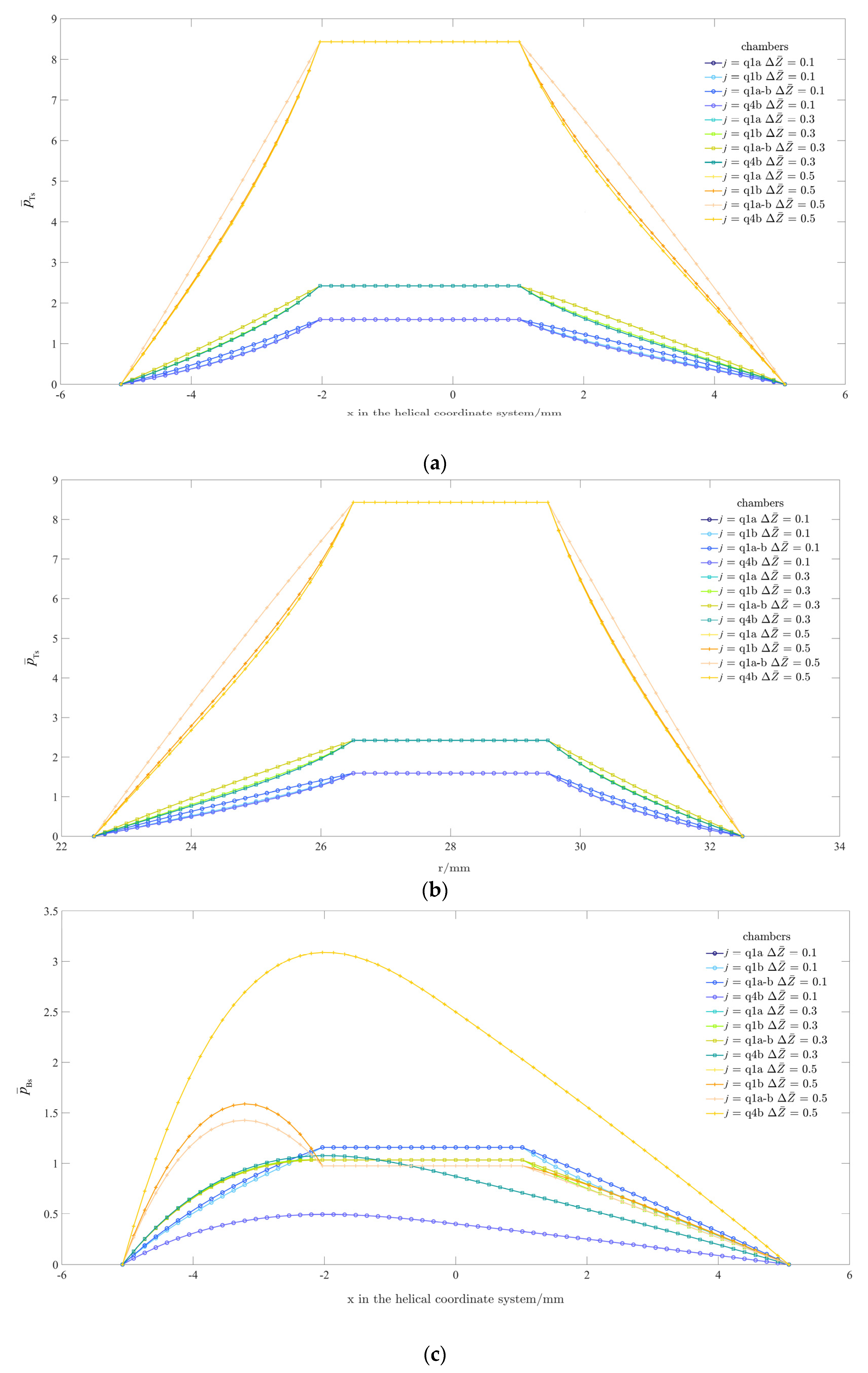
3.1. Flow-Field Pressure Analysis

The main geometric parameters of the system are listed in

Table 2. Main geometric parameters of the system.

Parameter	Value
$P$	25 mm
$\alpha$	10°
$h_{\mathrm{n}0}$	0.03 mm
$r_{\mathrm{m}}$	27.5 mm
$r_{\mathrm{i}}$	22.5 mm
$r_{\mathrm{ci}}$	26.5 mm
$r_{\mathrm{co}}$	29.5 mm
$r_{\mathrm{o}}$	32.5 mm

, and the numerical model of the flow fields is solved by MATLAB software.

The negative pressure values outside film-rupture boundary which is taken as 0 MPa [33], are set to zero, when the steady pressures are solved with MATLAB, but it is not necessary for those under the disturbed state to be processed in that way. It can be found in the calculation that the first-order pressure disturbances are solved based on the steady pressures, and the total pressures are less influenced by the second-order pressure disturbances than the others. Thus, the steady pressures can be taken as the main targets, when the pressure fields are analyzed.

Dimensionless pressure distributions of the flow fields based on the new method, are shown in Figure 3. The number of grid points in the $\mathit{x}$ direction is 100, and that in the $\mathit{s}$ direction is 360. $\Omega$ is $500 \mathrm{rm}$, is $0.4$, “$X,Y,Z$” is used to orientate the fluid particle, “$T$” represents the upper fields of the nut, and “$\mathrm{B}$” represents the lower fields, with “$Z_{\mathrm{d}}$” and “${\stackrel{•}{Z}}_{\mathrm{d}}$” indicating the first-order and second-order pressure disturbance, respectively, for example, “${\overline{P}}_{\mathrm{Ts}}$” denotes the dimensionless pressure of the upper flow fields of the nut in the steady state.

As mentioned in Section 2.1, the system is assumed to be oriented vertically, and the sealing surfaces of the upper and lower fields are named the upper sealing surfaces and the lower sealing surface, respectively. Besides, for the flow fields on either side of the nut, the sealing surfaces at the both ends of the four turns of helical fields with oil chambers are called the front sealing surface and the rear sealing surface, respectively, according to their locations relative to the coordinate origin O₁.

It can be concluded from Figure 3a,d that the nut is subjected to a downward driving force from the fluids, which is consistent with the actual condition mentioned in Section 2.1. Such a result is related to the regulating functions of the restrictors.

As shown in Figure 3a, a symmetrical drop around $r_{\mathrm{ci}}\le r\le r_{\mathrm{co}}$ occurs in the four turns of helical fields with oil chambers, and the pressure values in the front and rear sealing surfaces are close to zero. The flow-field pressures in Figure 3d show irregular change trends with variable gradients in the whole fields, especially in the front and rear sealing surfaces. Such irregular changes also obviously occur in the front and rear sealing surfaces in Figure 3c,e,f. The seemingly irregular changes mainly serve as a result of a combined effect of the torsion, lead angle, thread angle of the helix, and the centrifugal forces, and the effect is larger than that of the restrictors, especially when the fluids are squeezed ($\Delta \overline{Z}=0.4$). As far as the upper flow fields are concerned, the enlarged clearance results in weaker diffusions to the sealing surfaces, hence the pressures in the sealing surfaces in Figure 3a are too small to show the pressure gradients caused by the above factors.

It is found that the illustrations in Figure 4 and Figure 5 are not intuitive enough, and some less obvious changes are not easy to catch. Thus, as shown in, the variations of the steady pressures with $\Delta \overline{Z}$ in the $\mathit{x}$($\mathit{r}$) and $\mathit{\theta }$($\mathit{s}$) direction are solved to observe and analyze the pressure fields more intuitively.

There is a mixture of Couette flow and Poiseuille flow in this research [34]. The motion of the screw relative to the nut brings the Couette flow. Poiseuille flow exists not only between a chamber and the adjacent sealing surface, but also between adjacent oil chambers. When the clearance thickness is small, the Couette flow is dominant to maintain the pressures constant among different oil chambers, such as when $\Delta \overline{Z}=0.1,0.3$ in Figure 4a and $\Delta \overline{Z}=0.1,0.3,0.5$ in Figure 4b. Then, these chamber pressures do not vary in the helical direction until the clearance thickness increases to large enough. As is shown in Figure 4a, when $\Delta \overline{Z}=0.5$, not only are pressure differences between the oil chambers and the sealing surfaces shown, but also the pressure differences caused by such factors as torsion and the lead angle are reflected among different oil chambers, which demonstrates the effect of Poiseuille flow on the chamber pressures.

When $\Delta \overline{Z}\ne 0$, i.e., $\overline{\Delta h}\ne 0$, the reason why the pressures in the sealing surfaces in Figure 4a are so small has been explained in Figure 3. The fluids on the lower side of the nut are squeezed and then diffuse to the sealing surfaces, which is intensified with the increase of $\Delta \overline{Z}$. As shown in the sealing surfaces in Figure 4b, a few sharp increases in the yellow curve occur when $\Delta \overline{Z}$ is large enough.

The chambers contribute to the bearing capacity much greater than the sealing surfaces, which is achieved with the help of the restrictors. As is shown in Figure 4a,b, with the increase of $\Delta \overline{Z}$, the chamber pressures of the upper flow fields gradually increase, yet the lower ones decrease, which brings about a larger bearing capacity.

The pressures vary with $x$ (or $r$) in the steady state. The variations in the oil chambers are displayed Figure 5a–d, and those in the sealing surfaces are displayed in Figure 5e,f. As shown in Figure 5b,d,f, the positions of fluid particles are transformed from “$\mathit{sxy}$” to “$\mathit{O}\mathit{r}\mathit{\theta }{\mathit{\xi }}_3$” for more intuitive analyses.

According to Figure 2, “$j$” denotes a set of nodes in the $\mathit{s}$ direction. “$\mathrm{hssB}$” is the midpoint of pitch diameter helix of the front sealing surface, “ $\mathrm{q}1\mathrm{a}$” is the intersection $a$ of pitch diameter helix of the front sealing surface and the adjacent “Chamber 1”, “$\mathrm{q}1\mathrm{b}$” is the node $b$ of “Chamber 1” in Figure 2 “$\mathrm{q}1\mathrm{a}-\mathrm{b}$” is the node $a-b$ of “Chamber 1” in Figure 2, “$\mathrm{q}4\mathrm{b}$” is the intersection $b$ of pitch diameter helix of the rear sealing surface and the adjacent “Chamber 4”, and “$\mathrm{hssT}$”is the midpoint of pitch diameter helix of the rear sealing surface. The nodes at “$j$” denote all the particles which have a $s$-coordinate of “$j$” in the following article.

Compared to the others, the pressure values at “$\mathrm{q}1\mathrm{a}$” are close to those at “$\mathrm{q}4\mathrm{b}$”. For example, when $\Delta \overline{Z}=0.1$, the order of magnitude of the upper pressure differences between “$\mathrm{q}1\mathrm{a}$” and “$\mathrm{q}4\mathrm{b}$” reaches ${10}^{-7}$, leaving only a curve visualized in Figure 5a,b. Furthermore, the lower pressure values at “$\mathrm{q}1\mathrm{a}$”, “$\mathrm{q}4\mathrm{b}$”, “$\mathrm{hssB}$”, and “$\mathrm{hssT}$” are close to each other. For the same $\Delta \overline{Z}$, only one of the curves at “$\mathrm{hssB}$”and “$\mathrm{hssT}$” is visible in Figure 5e,f. Consequently, when the lower chamber pressures are analyzed, the pressures at “$\mathrm{q}1\mathrm{a}-\mathrm{b}$” and “$\mathrm{q}1\mathrm{b}$” can be selected as the main research objects.

As shown in Figure 5b, the pressures remain relatively stable in the chambers, but descend to the sealing surfaces in the ranges of $r_{\mathrm{i}}\le r\le r_{\mathrm{ci}}$ and $r_{\mathrm{co}}\le r\le r_{\mathrm{o}}$. When $\Delta \overline{Z}=0.1,0.3$, there are similar situations at “$\mathrm{q}1\mathrm{a}-\mathrm{b}$” and “$\mathrm{q}1\mathrm{b}$” in Figure 5d. With the growing of $\Delta \overline{Z}$, the descending slope of the pressures in the range of $r_{\mathrm{co}}\le r\le r_{\mathrm{o}}$ in Figure 5d becomes smaller. And when $\Delta \overline{Z}$ is large enough, a pressure jump occurs. For example, there is an obvious jump in the range of $r_{\mathrm{co}}\le r\le r_{\mathrm{o}}$ at “$\mathrm{q}1\mathrm{b}$” in Figure 5d, when $\Delta \overline{Z}=0.5$.

As mentioned in Figure 3 and Figure 4, the bearing capacity of the system mainly benefits from the regulations of the restrictors on the upper and lower chamber pressures. Furthermore, the pressures are also influenced by the torsion, lead angle and thread angle of the helix, and the centrifugal forces. Under the effect of these factors, the diffusions to the sealing surfaces are enhanced when the fluids in the gap are squeezed. As shown in Figure 5c,d, the regulation effects of the restrictors on the lower pressures are weakened by the diffusions. Meanwhile, with the enlarged clearance and the diffusions to the sealing surfaces, larger upper pressures are caused by the restrictors in Figure 5a,b. With the increase of $\Delta \overline{Z}$, the regulation effects of the restrictors are enhanced, then smaller decline ranges of the lower pressures in Figure 5c,d serve as a result of the combined effect of the restrictors, the torsion, lead angle and thread angle of the helix, and the centrifugal forces. In this situation, the increasing amplitudes of the upper pressures become larger in Figure 5a,b, which reflects the sensitivity of bearing capacity to $\Delta h$. Such a phenomenon is consistent with that mentioned inFigure 4.

The pressure values in the upper sealing surfaces are near zero according to Figure 3, thus they are not discussed in this part. As mentioned above, the pressures in the lower sealing surfaces increase when the fluids are squeezed; such changes are shown in Figure 3d–f, Figure 5e,f, under the combined influence of the torsion, lead angle and thread angle of the helix, and the centrifugal forces. The increasing amplitudes of the pressures become larger with the growing of $\Delta \overline{Z}$, as shown in Figure 5e,f. The reason why the pressures decrease to zero in the ranges of $r_{\mathrm{i}}\le r\le r_{\mathrm{ci}}$ and $r_{\mathrm{co}}\le r\le r_{\mathrm{o}}$ is that the fluids diffuse to the root and crest, and the tops of the hills in Figure 5f are found to be closer to the position with a radius of $r_{\mathrm{co}}$, largely due to the centrifugal forces. Such explanations can also be applicable to the conditions at “$\mathrm{q}1\mathrm{a}$” and “$\mathrm{q}4\mathrm{b}$” in Figure 5d.

3.2. Feasibility Evaluation Based on the Bearing Capacity

The aerostatic leadscrew system in [6] is solved numerically based on the method proposed in this research, and the simulation results are compared with the experimental data [6] to evaluate the feasibility of the new method.

The comparisons between the simulation results and experimental data are shown in Figure 6, in which the experimental data for a two-pitch travel are represented by the yellow ★, and the simulation results at $\Omega =120 \mathrm{rpm}$, $\Omega =100 \mathrm{rpm}$, and $\Omega =60 \mathrm{rpm}$ are represented by the red ▲, blue ●, and green ◆, respectively.

It is found that the numerical predictions agree well with the experimental data qualitatively. However, from a quantitative point of view, there are still some deviations between them. It is inevitable that the data points in the two cases would not coincide. Because the information about the speeds were not provided, the experimental results were not collected until the system stopped running and kept steady, rather than real-time like the simulation results. Besides, it is also necessary to consider the divergences caused by the experimental environments, operating methods, geometric errors, etc.

As shown in Figure 6, when $1.4 \mathsf{\mu }\mathrm{m}\le \Delta Z\le 4.8 \mathsf{\mu }\mathrm{m}$, the larger the value of $\Omega$, the closer the simulation results are to the experimental ones, however, the situation is the opposite in the range of $\Delta Z<1.4 \mathsf{\mu }\mathrm{m}$, which is closely associated with the collection method of the experimental data. Among the simulation data, the red ▲ data are closer to the yellow ★ ones with a maximum difference of about $1.8N$, which is approximately $14\%$ of the corresponding experimental value.

Therefore, the new method can be considered to be feasible, and the results can provide references for predicting the actual characteristics of the system.

4. Conclusions

In this research, a new method is attempted to overcome the shortcomings of the existing modeling methods of the hydrostatic and aerostatic leadscrews, and a screw-driven hydrostatic leadscrew is selected as the main research object to describe the proposed method.

In the new method, the follow-up coordinate system is adjusted to adapt to the boundaries of the flow fields, which makes the calculations of $h$ and $\Delta Z$ more accurate. Furthermore, compared with those approximations in the cylindrical coordinate system, the description in the helical coordinate system can provide a better reappearance of the actual shape of the flow fields.

Through the analyses about the pressure fields in Section 3.1, it can be found that the influences of the torsion, lead angle, and thread angle of the helix are taken into consideration in this research, and the actual flow fields are reflected well by the simulation results based on the new method.

The experiments on an aerostatic leadscrew in [6] are employed to discuss the feasibility of the new method in Section 3.2. In the numerical calculations, known parameters in [6] are set to keep the consistency between the conditions of the experiment and the simulations, and $\Omega$ is set in different ranges to reduce the interferences caused by the data collection method. In Figure 6, the red curve shows a better consistency with the yellow target curve than the others, and the relative errors between them are mostly within $10\%$, demonstrating that the new modeling method is possessed of good practicability and generality.

The method in this research is suitable for all helical gap flow fields created by a screw-driven screw-nut pair, and some adjustments may occasionally be made on the assumptions in (1)–(7) or the fluid governing equations in Section 2.1 to satisfy different lubrication media or applications. Although the assumptions are made for the sake of simplicity in this research, the proposed method provides a new way of thinking for the flow-field modeling of various leadscrews with fluids as lubrication media. With the adjustments of the flow-field models, not only various types of fluid-lubricated leadscrews, but also more complicated flow-field properties and phenomena can be solved and analyzed in future researches.

References

1. Wertwijn, G.; Kolarich, S. Selecting a hydrostatic lead screw. Power Transm. Des. 1967, 61, 9. [Google Scholar]
2. Matataro, T.; Akira, Y.; Shunichi, K.; Katsuyuki, T. A Study on Hydrostatic Lead Screws (1st Report). J. Jpn. Soc. Precis. Eng. 1981, 47, 1504–1509. [Google Scholar]
3. Matataro, T.; Akira, Y. A Study on Hydrostatic Lead Screws (2nd Report). J. Jpn. Soc. Precis. Eng. 1982, 48, 1341–1347. [Google Scholar]
4. Satomi, T.; Yamamoto, A. Studies on the Aerostatic Lead Screws (1st Report). J. Jpn. Soc. Precis. Eng. 1984, 50, 975–980. [Google Scholar] [CrossRef] [Green Version]
5. Satomi, T.; Yamamoto, A. Studies on the Aerostatic Lead Screws (2nd Report). J. Jpn. Soc. Precis. Eng. 1985, 51, 1915–1920. [Google Scholar] [CrossRef] [Green Version]
6. Zhao, P.; Satomi, T. Study on Aerostatic Lead Screw. J. Jpn. Soc. Precis. Eng. 2007, 73, 1350–1355. [Google Scholar] [CrossRef] [Green Version]
7. Shen, T. Research on Aerostatic Leading Screw. Master’s Thesis, Harbin Institute of Technology, Harbin, China, 2008. [Google Scholar]
8. Luo, S.; Zhao, S. Liquid Nut for High Speed Transmission System. Mach. Tool Hydraul. 2008, 36, 327–328. [Google Scholar]
9. Zhong, W. Performance Research on Hydrostatic Lead Screws with Spool-Type Restrictors. Master’s Thesis, Shandong University, Jinan, China, 2017. [Google Scholar]
10. Xin, Z. Design and Dynamic Analysis of Full Static Pressure Double Drive Screw Transmission System. Master’s Thesis, Shandong University, Jinan, China, 2020. [Google Scholar]
11. El-Sayed, H.R.; Khataan, H. The exact performance of externally pressurized power screws. Wear 1976, 30, 237–247. [Google Scholar] [CrossRef]
12. El-Sayed, H.R.; Khataan, H. The running performance of externally pressurized power screws. Wear 1976, 39, 285–306. [Google Scholar] [CrossRef]
13. El-Sayed, H.R.; Khataan, H. A suggested new profile for externally pressurized power screws. Wear 1975, 31, 141–156. [Google Scholar] [CrossRef]
14. Zhang, Y.; Chen, S.; Lu, C.; Liu, Z. Performance Analysis of Capillary-Compensated Hydrostatic Lead Screws with Discontinuous Helical Recesses Including Influence of Pitch Errors in Nut. Tribol. Trans. 2016, 60, 974–987. [Google Scholar] [CrossRef]
15. Zhang, Y.; Lu, C.; Ma, J. Research on two methods for improving the axial static and dynamic characteristics of hydrostatic lead screws. Tribol. Int. 2017, 109, 152–164. [Google Scholar] [CrossRef]
16. Susumu, O. A Prototype Production of Aerostatic Lead Screw with Resin Molded Bearing Surfaces and Performance Evaluation. J. Jpn. Soc. Precis. Eng. 2015, 81, 570–575. [Google Scholar]
17. LU, Z.; YU, X. Research on the Porous Aerostatic Lead Screw and Nut. Mach. Tool Hydraul. 2007, 35, 34–36. [Google Scholar]
18. Vortmeyer-Kley, R.; Gräwe, U.; Feudel, U. Detecting and tracking eddies in oceanic flow fields: A Lagrangian descriptor based on the modulus of vorticity. Nonlinear Proc. Geoph. 2016, 23, 159–173. [Google Scholar] [CrossRef] [Green Version]
19. Zhang, H.; Hao, H.; He, L.; Gong, M. Single-mode annular chirally-coupled core fibers for fiber lasers. Opt. Commun. 2018, 410, 297–304. [Google Scholar] [CrossRef]
20. Gelfgat, A. Instability of steady flows in helical pipes. Phys. Rev. Fluids 2020, 5, 103904. [Google Scholar] [CrossRef]
21. Germano, M. On the effect of torsion on a helical pipe flow. J. Fluid Mech. 1982, 125, 1–8. [Google Scholar] [CrossRef] [Green Version]
22. Bolinder, C.J. Curvilinear coordinates and physical components: An application to the problem of viscous flow and heat transfer in smoothly curved ducts. J. Appl. Mech. 1996. [Google Scholar] [CrossRef]
23. Tuttle, E.R. Laminar flow in twisted pipes. J. Fluid Mech. 2006, 219, 545–570. [Google Scholar] [CrossRef]
24. Ma, W.; Cui, J.; Liu, Y. Improving the pneumatic hammer stability of aerostatic thrust bearing with recess using damping orifices. Tribol. Int. 2016, 103, 281–288. [Google Scholar] [CrossRef]
25. Miyan, M. Different phases of Reynolds equation. Int. J. Appl. Res. 2016, 2, 140–148. [Google Scholar]
26. Al-Ghussain, L.; Bailey, S.C.C. An approach to minimize aircraft motion bias in multi-hole probe wind measurements made by small unmanned aerial systems. Atmos. Meas. Tech. 2021, 14, 173–184. [Google Scholar] [CrossRef]
27. Hnat, S.K.; van Basten, B.J.H.; van den Bogert, A.J. Compensation for inertial and gravity effects in a moving force platform. J. Biomech. 2018, 75, 96–101. [Google Scholar] [CrossRef] [Green Version]
28. Abass, B.A.; Muneer, M.A.A. Static and Dynamic Performance of Journal Bearings lubricated With Nano-Lubricant. Assoc. Arab Univ. J. Eng. Sci. 2018, 25, 201–212. [Google Scholar]
29. Chen, X.; Zeng, L.; Zheng, F. Friction performance and optimisation of diamond-like texture on hydraulic cylinder surface. Micro. Nano Lett. 2018, 13, 1001–1006. [Google Scholar] [CrossRef]
30. Chin, D.; Kim, K.; Yoon, M. Lubrication Behavior of Slider Bearing with Square Pocket Surface. J. Korean Soc. Manuf. Process Eng. 2017, 16, 119–125. [Google Scholar] [CrossRef]
31. Huang, M.; Xu, Q.; Li, M.; Wang, B.; Wang, J. A calculation method on the performance analysis of the thrust aerostatic bearing with vacuum pre-load. Tribol. Int. 2017, 110, 125–130. [Google Scholar] [CrossRef]
32. Premoli, A.; Rocchi, D.; Schito, P.; Tomasini, G. Comparison between steady and moving railway vehicles subjected to crosswind by CFD analysis. J. Wind Eng. Ind. Aerod. 2016, 156, 29–40. [Google Scholar] [CrossRef]
33. Su, H. Determining the Value of Pressure in the Cavitation Zone for Steady-state Journal Bearing. China Mech. Eng. 2007, 88–90. [Google Scholar] [CrossRef]
34. Zehra, I.; Kousar, N.; Rehman, K.U. Pressure dependent viscosity subject to Poiseuille and Couette flows via Tangent hyperbolic model. Phys. A 2019, 527, 121332. [Google Scholar] [CrossRef]
Figure 1. Modeling diagram based on the helical coordinate system. (a) Schematic diagram; (b) modeling of fluid domain; (c) “ n - n ” of the screw; (d) initial section; (e) velocity relations.
Actuators 10 00190 g001
Figure 2. Axial projection of the chamber distributions.
Actuators 10 00190 g002
Figure 3. Pressure distributions of the flow fields based on the method proposed in Section 2. (a) P ¯ Ts ; (b) P ¯ TZ d ; (c) P ¯ T Z d ; (d) P ¯ Bs ; (e) P ¯ BZ d ; (f) P ¯ B Z d .
Actuators 10 00190 g003
Figure 4. The variations of the steady pressures in the θ direction. (a) P ¯ Ts ; (b) P ¯ Bs .
Actuators 10 00190 g004
Figure 5. The variations of the steady pressures in the x (or r ) direction. (a) P ¯ Ts , x , chambers; (b) P ¯ Ts , r , chambers; (c) P ¯ Bs , x , chambers; (d) P ¯ Bs , r , chambers; (e) P ¯ Bs , x , sealing surfaces; (f) P ¯ Bs , r , sealing surfaces.
Actuators 10 00190 g005aActuators 10 00190 g005b
Figure 6. Comparisons between the simulation results and experimental data.
Actuators 10 00190 g006