Article

Design and Optimal Control of a Multistable, Cooperative Microactuator

1
Chair of Control Engineering, University of Augsburg, Eichleitnerstraße 30, D-86159 Augsburg, Germany
2
Research Group for Modelling and Simulation of Mechatronic Systems, Jade University of Applied Sciences, D-26389 Wilhelmshaven, Germany
*
Authors to whom correspondence should be addressed.
Actuators 2021, 10(8), 183; https://doi.org/10.3390/act10080183
Submission received: 12 July 2021 / Revised: 29 July 2021 / Accepted: 31 July 2021 / Published: 4 August 2021
(This article belongs to the Special Issue Cooperative Microactuator Systems)

Abstract

:
In order to satisfy the demand for the high functionality of future microdevices, research on new concepts for multistable microactuators with enlarged working ranges becomes increasingly important. A challenge for the design of such actuators lies in overcoming the mechanical connections of the moved object, which limit its deflection angle or traveling distance. Although numerous approaches have already been proposed to solve this issue, only a few have considered multiple asymptotically stable resting positions. In order to fill this gap, we present a microactuator that allows large vertical displacements of a freely moving permanent magnet on a millimeter-scale. Multiple stable equilibria are generated at predefined positions by superimposing permanent magnetic fields, thus removing the need for constant energy input. In order to achieve fast object movements with low solenoid currents, we apply a combination of piezoelectric and electromagnetic actuation, which work as cooperative manipulators. Optimal trajectory planning and flatness-based control ensure time- and energy-efficient motion while being able to compensate for disturbances. We demonstrate the advantage of the proposed actuator in terms of its expandability and show the effectiveness of the controller with regard to the initial state uncertainty.

1. Introduction

Multistability is an important system property found in a variety of microactuators and corresponds to possessing multiple stable actuator positions. While it is most commonly used in switches with two stable resting positions, extending the number of equilibrium points opens up new possibilities in the functionality and application flexibility of microsystems. Especially for actuators with large working ranges, which are currently the focus of research, multistability may prove useful.
In order to enlarge the operating ranges of microactuators, mechanical connections resulting in large restoring forces have to be overcome. Therefore, a considerable number of actuator concepts have been proposed, which can be distinguished in particular on whether the entire actuator or a single object is moved. The former includes impact mechanisms, which generate a stepwise motion by repeated impact between an internal mass and a stopper and can be realized using different actuation principles [1,2,3]. Stick-slip actuators also move in small steps, but exploit different friction effects. Therefore, movements of both high precision [4] and large displacements [5] are possible. Progress has also been made in terms of new concepts, such as legged platforms, comparable to a linear motor [6,7]. In these approaches, the actuator is driven by traveling waves, generated by piezoelectric MEMS. Large travel ranges can also be achieved by more complex setups, such as the microrobot of Floyd et al. [8]. In these cases, there are no restoring forces driving the actuator back into its initial state. Thus, they are multistable since every position corresponds to a steady state when no external input is applied.
For many applications, however, the motion of a single passive object is sufficient. This typically results in less complex designs, simplifying the assembly process. In the simplest case, a small object, e.g., a magnet, can be used for a bistable switching application [9], or it is moved between these two stable positions using feedback control [10]. The advantage of the magnetic principle lies in the fact that both equilibrium positions are asymptotically stable in their vicinity, even without further input. Other typical applications include linear micro motors [11,12] and micro conveyor systems [13]. As proposed by Poletkin et al., conveyor systems can also be realized by arrays of inductive suspensions [14]. These have in common that they are based on levitation of the moved object, but need constant energy input to generate asymptotically stable equilibria. Another important criterion corresponds to the achieved degree of freedom (DoF). Without adaption, these actuators can only be used for planar movements and thus are strongly limited in the vertical direction.
In order to allow a flexible application in both the horizontal and vertical directions, we previously presented a magnetic actuator moving a cylindrical permanent magnet with one DoF [15]. To this end, finite element models (FEM) were used to calculate the magnetic forces, and their complexity was reduced by different approaches, i.e., a lookup-table, a semi-analytical compact model, and a parametric reduced order model [16,17]. These methods were then compared in terms of simulation time and accuracy, and their usefulness for a controller design was demonstrated. The actuator consists of permanent magnetic rings, generating two stable equilibrium positions: a lower one in contact with a piezoelectric stack actuator, and a second one located at a predefined height, where the magnetic object is stably levitated. Fast and efficient transient motion between these positions is handled by cooperation of the stack actuator, enabling a fast initial acceleration of the magnet to be moved, and a controlled catch at the second stable equilibrium, using electromagnets.
A major drawback lies in the merely bistable design and the restriction of the movable object to remain below the center of the electromagnetic solenoid, due to the limited controllability. In this work, we therefore aim to extend the proposed design by multiple solenoids and ring magnets, such that a greater number of resting positions is generated. In order to reduce electrical currents within the solenoids, a cooperative mechanism between the piezoelectric actuator and multiple solenoids is exploited. Moreover, an optimal control strategy is used to find a trade-off between low solenoid currents and time-optimal transitions. The effectiveness of the control scheme is demonstrated in the simulation, and the expandability of the actuator is discussed. The advantage of the proposed concept lies in its extensibility to larger working ranges as well as the generalizable control algorithm for an arbitrarily extended actuator.

2. Methods

The microactuator setup investigated in this work consists of a movable, permanent magnetic proof mass guided by a glass tube, a piezoelectric stack actuator, two permanent ring magnets and two solenoids. In contrast to our previous work [15], the second magnet is used to imprint a second levitating equilibrium position, rather than weakening the field of the first magnet. The additional solenoid allows a less restrictive motion range of the proof mass, which was an issue of the initial setup. The basic design is sketched in Figure 1. The grayed-out part illustrates its expandability, which is discussed Section 3.1.
The working principle is as follows: Initially, the proof mass is placed on top of the stack actuator, which corresponds to the lower resting position. In order to obtain an impulse-like acceleration, the inverse piezoelectric effect is used to kick the cylindrical magnet upwards. Subsequently, the electromagnetic solenoids are switched on and cooperatively catch it at the desired resting position in a controlled way. Since these positions are asymptotically stable by design, the proof mass is suspended without the need for further energy input. Concerning the transitions between the levitation equilibria, as well as the downwards motion, mere electromagnetic actuation is applied. The control objective is to achieve fast movements with minimum solenoid current. For this purpose, a mathematical system model containing all relevant effects is derived, and an optimal model-based control strategy is presented.

2.1. Modeling

The overall system can be described by the dynamics of each individual component and the respective couplings between them. The model is adapted from [15] and generalized for an arbitrary number of magnets and solenoids. Let us assume that the setup comprises m ring magnets and n electromagnets. The dynamic behavior of the current i k ( t ) of the k-th solenoid with inductance L k , wire resistance R k and input voltage u k ( t ) is then given by the following:
L k d i k ( t ) d t = u k ( t ) + u ind , k ( t ) R k i k ( t ) ,
where u ind , k ( t ) is the voltage induced due to the change of electric current within the other solenoids. Given the coupling inductance L j , k describing the influence of the j-th solenoid on the k-th solenoid, the induced voltage is defined by the following:
u ind , k ( t ) = j k n L j , k d i j ( t ) d t .
The current of each solenoid affects the proof mass with vertical position z ( t ) in terms of an electromagnetic force F em , k ( z , i k ) , which is defined below in (9).
Similar to [18], we assume the piezoelectric actuator to behave like a linear second order system but neglect the hysteresis effect. Although the literature suggests more complex, nonlinear dynamics [19,20], this approximation seems justified, due to the short time of contact between the piezo and the proof mass. Therefore, we model the deformation d ( t ) of the piezo as follows:
M d ¨ ( t ) = M g c A d · ( t ) k A d ( t ) F c ( t ) + F u ( t ) ,
with the effective mass M, gravitational acceleration g, damping coefficient c A and stiffness k A . The force that results in the deformation by applying a voltage u A ( t ) is considered by F u ( t ) and the interaction with the proof mass corresponds to the contact force F c ( t ) . In order to describe F u ( t ) in dependence of the applied voltage, we consider the static piezoelectric behavior. As proposed in [21], we use a linear relation between the force, deflection, and input voltage, resulting in the following:
F ext = k A d + k A d 33 n A u A = k A d + F u
with the piezoelectric constant d 33 and the number of stack layers n A of the piezoactuator. Here, the external forces including the gravitational force are summarized in F ext . Due to the stiffness term, the maximum force, i.e., the blocking force F max , is achieved by applying the maximum voltage U max in case of a zero displacement d = 0 . By inserting these values into (4), we obtain the following expression:
k A d 33 n A = F max U max
and thus simplify the piezoelectric force as the following:
F u ( t ) = F max U max u A ( t ) .
The magnet motion can be summarized to the following:
m z ¨ = k = 1 m F pm , k ( z ) + k = 1 n F em , k ( z , i k ) + F c ( z , z · , d , d · ) c f z · m g ,
with the force F pm , k ( z ) corresponding to the k-th ring magnet, gravitation according to the proof mass m and friction with the coefficient c f . Note that the time dependencies are neglected for readability. The magnetic forces can further be decomposed into position-dependent shape functions f ˜ pm , k ( z ) , f ˜ em , k ( z ) and proportional weighting factors as the following [22,23]:
F pm , k ( z ) = B r , pm , k B r , p f ˜ pm , k ( z ) = f pm , k ( z )
F em , k ( z , i ) = i k B r , p f ˜ em , k ( z ) = i k f em , k ( z ) .
The values B r , p , B r , pm , k are the magnetic remanences of the proof mass and ring magnets. The forces are precomputed numerically with ANSYS® Maxwell [24] and are implemented as spline-interpolated lookup tables.
The contact force F c ( z , z · , d , d · ) between the movable mass and the piezoelectric actuator is approximated by a viscoelastic formulation adapted from Specker et al. [25]. Thus, by softening the contact characteristic, we mathematically allow a small penetration s ( t ) = z ( t ) d ( t ) of the piezo surface being counteracted by a force. The adapted approach is comparable to a spring with nonlinear contact stiffness, or activation function, R a ( s ) , but additionally takes into account energy loss at the impact, using a power function R p ( s · ) . The contact force can then be computed by the following:
F c ( s , s · ) = R a ( s ) R p ( s · ) s · .
Since the original formulation of Specker et al. considers possible material breach within R p ( s · ) and R a ( s ) , which are not necessary in this work, the individual functions are adapted. Thus, we use the power function as follows:
R p ( s · ) = s · 2 log cosh ( r d s · ) 2 r d
with damping parameter r d and the following piecewise activation function:
R a ( s ) = 0 , if s 0 k c 2 4 F s 2 , if 2 F k c < s < 0 k c s F , otherwise .
Here, k c and F are design parameters corresponding to the contact stiffness and the force at the transition between the quadratic and linear parts. These values can be adjusted to achieve realistic impact behavior while being feasible for a standard numerical ODE-solver. Finally, we define the state vector x ( t ) comprising all individual state variables, i.e., the following:
x ( t ) = z z · i 1 i 2 i n d d · .
It is important to mention that the presented model is not assumed to be a highly accurate representation of the later setup. Instead, it is necessary in an early stage of system design when no prototype is available. It is deployed to analyze system properties and to design component dimensions and controller architectures.

2.2. Trajectory Planning and Control

Based on the system model, we now derive a control strategy that efficiently exploits the cooperative mechanism in order to minimize the transient time and input current. To this end, we consider the kick and catch motions as separate parts. First, the piezoelectric kick is used to accelerate the proof mass. Subsequently, the controller is switched on, transferring the new initial state, i.e., the terminal state of the kick, into the desired final state.

2.2.1. Piezoelectric Kick

Accelerating the magnet by electromagnetic actuation needs large currents. Moreover, this process is slowed down due to restrictions in the maximum current. In case of the presented actuator, we therefore use a mechanical kick force to start the upwards motion. This is achieved by applying a voltage spike to the piezoelectric actuator, resulting in a large deformation of its surface and thus a fast acceleration of the proof mass. For an efficient kick, a fast voltage rise is important, while further input after the initial acceleration is unnecessary. These requirements are fulfilled by an input voltage trajectory following the course of time expressed by the following:
u A ( t ) = U p U ^ exp t τ 1 exp t τ 2 ,
which will be used with the time constants τ 1 = 0.1   m s , τ 2 = 2.5   m s in the remainder of this work. Here, U p U max corresponds to the predefined peak voltage, and U ^ is a normalizing factor given by the following:
U ^ = τ 2 τ 1 τ 1 ( τ 1 τ 2 ) 1 τ 2 τ 1 τ 2 ( τ 1 τ 2 ) 1 .
Note that for the practical setup, only the time course of the initial steep edge is important, and the exact voltage may be realized differently. Moreover, instead of an analytical approach, an experimental setup is preferable for the identification of the actual proof mass acceleration.
After the time T kick , the electromagnets are switched on. We therefore use the terminal position and velocity z ( T kick ) , z · ( T kick ) as initial values for the following control approach.

2.2.2. Flatness-Based Control

Feedback control is applied to obtain smooth motions between the resting positions and to compensate for potential disturbances. The states of the proof mass and the solenoids are independent, with exception of the impact during the downwards motion. Hence, we neglect the variables d ( t ) and d · ( t ) for now, and thus consider only the magnetic part. We now have to define a distinct relation as follows:
i k ( t ) = g F em ( t )
according to (9), to compute the separate currents i k from the overall electromagnetic force. Hence, the system is flat with respect to the output variable z, which is advantageous for the control approach. Flatness means that all states and inputs can be reconstructed by means of the output variable and a finite number of its derivatives. This enables us to choose a feasible, sufficiently smooth reference motion z ref and inversely compute the state and input trajectory using this output and its derivatives [26].
It is important to mention that the relation (16) is not automatically fulfilled by the system. However, we can achieve this property by utilization of an appropriate cascade structure, which will then be combined with the flatness-based controller. For this purpose, the system is split up into two parts: the linear system comprising the solenoids, and the nonlinear part describing the relation between electromagnetic force and proof mass position. These partial systems are coupled by expression (9). The overall control approach is shown in Figure 2 and is explained in detail in the following.
In order to achieve the desired flatness property, we first have to ensure that the individual currents i k follow a reference w k , which fulfills the necessary condition (16). Therefore, an inner control loop for the solenoid system is used. We collect the solenoid inputs and currents within the vectors u and i . According to Equations (1) and (2), the linear partial system can compactly be written as the following:
L d i ( t ) d t = u ( t ) R i ( t ) ,
with the invertible, symmetric inductance matrix L and diagonal resistance matrix R . We can now imprint n eigenvalues p i = [ p 1 , p 2 , , p n ] on the system by computing an appropriate feedback matrix K i by pole placement and using the control law as follows:
u ( t ) = K i i ( t ) + S i w i ,
as seen in Figure 2a. Here, the subscript i denotes the correspondence to the solenoid control loop. The vector w i is the reference variable for the solenoid currents and S i is a prefilter, which in our case is calculated by the following:
S i = L ( K i + R ) 1 L 1 1 .
The prefilter is used to ensure stationary accuracy. For more detailed information on multivariable linear control, the reader is referred to [27].
A second controller stabilizing the proof mass motion along a given trajectory is necessary. Due to the flatness property, dynamic feedback linearization can be used, compensating the nonlinearities within the overall system [28]. For this purpose, the following state transformation from the nonlinear state x to a linear state ξ is necessary:
x ( t ) = z z · i 1 i n a b c T ( x ) a b c ξ ( t ) = z z · z ¨
This can be found by reformulating (7). So far, there does not yet exist a distinct back transformation needed for the linearization approach. In other words, given z, z · and z ¨ , there exist arbitrarily many input combinations i ( t ) leading to the same electromagnetic reference force F em , ref and therefore to z ¨ . To overcome this, an artificial expression is derived, distinctly defining the currents i ( t ) in dependence of a single input parameter r ( t ) , and therefore also the reversible transformation from [ z z · r ] to [ z z · z ¨ ] .
Since we aim to minimize the currents, the solution at a single time instant is obtained by solving the following optimization problem:
min i k , k = 1 , , n k = 1 n i k 2 ( t )
s . t . k = 1 n i k ( t ) f em , k ( t ) = F em , ref ( t ) .
This results in the following:
i k ( t ) = r ( t ) f em , k ( t ) ,
with the new single input
r ( t ) = F em , ref ( t ) k = 1 n f em , k 2 ( t ) .
That means that the transformation law (23) distributes the currents in such a way that the solenoid with the largest effect on the proof mass contributes the most to achieve the necessary force. This is a large improvement, compared to the previous solution with a single electromagnet, where a singularity occurs when the movable magnet coincides with the center of the solenoid [15]. It can be seen that the desired relation (16) between the electrical currents and the electromagnetic force results from Equations (23) and (24). The transformed system then has the following dynamics:
ξ · ( t ) = f ( ξ , ν ) = 0 1 0 0 0 1 0 0 0 ξ ( t ) + 0 0 1 ν ( t )
with virtual input ν corresponding to the third motion derivative z ( 3 ) . It is now possible to find a linear control law for ν and stabilize the complete nonlinear system by the inverse computation of w i from ν . This can be achieved by derivating (7) over time, inserting Equations (17)–(19) and subsequent reorganization. Note that for the reference currents w i , the same transformation (23) to a single input r ref has to be performed. Instead of Equation (24), this is given by the inversely computed feedback linearization as follows:
r ref ( t ) = m ν + c f z ¨ ( F pm + i f em ) z · + f em L 1 ( R + K i ) i f em L 1 ( R + K i ) f em ,
which corresponds to Figure 2b. The following trajectory is now achieved by the control law:
ν ( t ) = z ref ( 3 ) + K z ξ ref ( t ) ξ ( t )
with an at least twice differentiable trajectory z ref that fulfills the transformed initial condition ξ 0 = T ( x 0 ) . For the computation of matrix K z , we again use pole placement. The controller of the outer control loop based on the state transformation (20) is labeled as Figure 2c. Given the flatness-based controller, it now remains to find suitable trajectories z ref ( 3 ) and ξ ref , which is the goal of the following trajectory planner.

2.2.3. Optimal Trajectory Planning

We aim to find motions that efficiently enable the proof mass to switch between the equilibrium positions, while also taking into account the initial state after the kick motion. Without loss of generality, we assume an arbitrary but known initial state ξ 0 = ξ ( t 0 ) at time t 0 = 0 . The goal is to find a sufficiently smooth trajectory, transferring the nonlinear system into the final state ξ f over the transition time T f .
In general, this can be achieved by connecting the initial and final state of a single transition with a polynomial, matching the initial and final conditions of the appropriate order. However, this may result in undesired oscillation and overshooting, comparable to the overfitting problem of neural networks. Instead, we use an optimization-based method with the goal to find trajectories with a low input current and short transition time, minimizing the cost function
J ( T f , i ) = w 1 T f + w 2 0 T f i ( t ) i ( t ) d t
with weighting factors w 1 and w 2 . To this end, we parameterize the trajectory using the parameter vector σ = [ σ 0 , σ 1 , , σ s ] . The optimization problem is then described by the following:
min T f , σ J ( T f , i )
s . t . ξ · ( t ) = f ( ξ , ν )
ξ ( 0 ) = ξ 0
ξ ( T f ) = ξ f ,
where (30) corresponds to the linear dynamics (25), and (31) and (32) are the initial and final state conditions. The time integral in (28) is approximated by the following:
0 T f i ( t ) i ( t ) d t T s j = 0 q i ( j T s ) i ( j T s )
with sampling time T s = T f / q . Moreover, we directly optimize the linear system input ν . The minimization problem is highly nonlinear due to the relation between the electrical currents and the linear motion. It is a known issue that for nonlinear problems, gradient-based optimization algorithms strongly depend on the initial parameterization and can get stuck in unsuited local minima. Therefore, Bergman et al. [29] proposed to initialize the motion with a predefined, suboptimal trajectory. We adapt this idea by superimposing a controller-based trajectory ν ctrl , further denoted as nominal trajectory, with the output ν opt of the optimization algorithm, that is, the following:
ν ( σ , t ) = ν ctrl ( t ) + ν opt ( σ , t ) .
For the nominal trajectory, we aim to find a preferably smooth function, connecting the initial and final states. Since each individual transition, with exception of the ones including the initial kick, begins and terminates in a state with zero velocity and acceleration, we choose a 5th order polynomial as the nominal trajectory. In the case of initial velocities, however, this function can result in a large overshoot, making it unusable for the motions with a piezoelectric kick. In order to remedy this issue, we use the analytic expression as follows:
ν ctrl ( t ) = λ 1 3 a e λ 1 t λ 2 3 b e λ 2 t λ 3 3 c e λ 3 t
for these trajectories, which can be found by the inverse Laplace transform of a stable, non-oscillating linear third-order system. Here, λ l > 0 , l = 1 , 2 , 3 correspond to predefined damping coefficients, and a, b, c are computed such that the initial conditions ξ 0 are fulfilled. Consequently, the initial values of the three time integrals of ν opt have to be zero. We know from Section 2.2.2 that the desired trajectory has to be at least twice differentiable. Thus, we can define ν opt to be a piecewise constant function as follows:
ν opt ( σ , t ) = σ s , s T h t < ( s + 1 ) T h .
For a better understanding of such a superimposed trajectory, an example is visualized in Figure 3.
The number of time intervals T h can be chosen arbitrarily, but have to be at least three. This is due to the fact that the controller trajectory is used for meeting the initial conditions, but its state transition only asymptotically approaches the desired final state ξ f . In order to compensate the deviation, the three last parameters σ k are fixed and cannot, therefore, be optimized. Their values can be obtained by solving a system of linear equations and are therefore not discussed in detail. The advantage of the superposition-based optimization is that, in general, acceptable solutions are obtained while the parameters can simply be initialized with zeros.
However, when the proof mass comes in contact with the stack actuator, numerical issues can arise during the optimization to the lower resting position. The most acceptable results, also in terms of computational time, are achieved by computing the inverted problem, that is, optimizing the motion starting at ξ f and ending up in ξ 0 . Subsequently, the resulting state trajectory has to be mirrored with respect to time, and the sign of every even derivative must be switched before evaluating the cost function.
Finally, for the utilization of an optimization toolbox based on symbolic calculations, the lookup-table for the magnetic forces cannot be implemented. To this end, we use a single layer radial basis function (RBF) neural network to obtain an analytical approximation. See Wu et al. [30] for a more general view on RBF networks. In our case, we use the approximator as follows:
F pm ( z ) μ = 1 η α μ exp z γ μ β 2 ,
which corresponds to a superposition of η Gaussian functions with respective center γ μ and weighting factor α μ . The parameter β adjusts the width of the basis functions and is chosen identically for each function. We then distribute the center points equidistantly throughout the relevant z-space. Since Equation (37) linearly depends on the remaining parameters α μ , we can use linear regression to fit the approximator to the data. The same method can be used for f em , k .

3. Results

We now combine the theoretical methods of the previous sections and demonstrate their usability. To this end, we first discuss the multistability and expandability property of the microactuator. This will facilitate the understanding of the subsequent simulation results of the control approach. All results were obtained using MATLAB® [31], with the exception of the magnetic forces, which were computed with ANSYS® Maxwell [24]. The optimization problem was solved using CasADi [32] with the solver IPOPT [33].

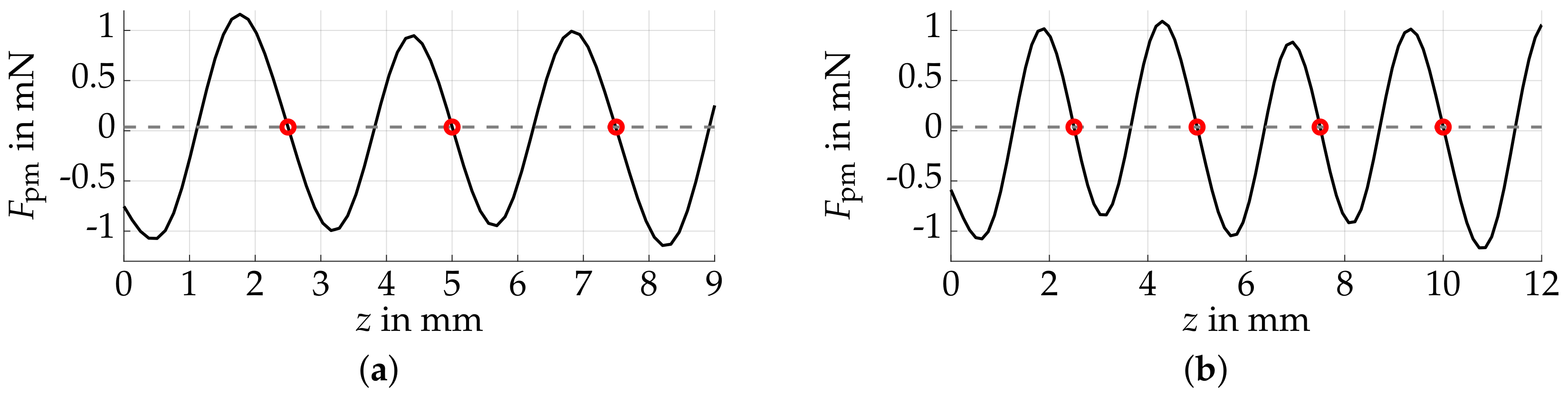
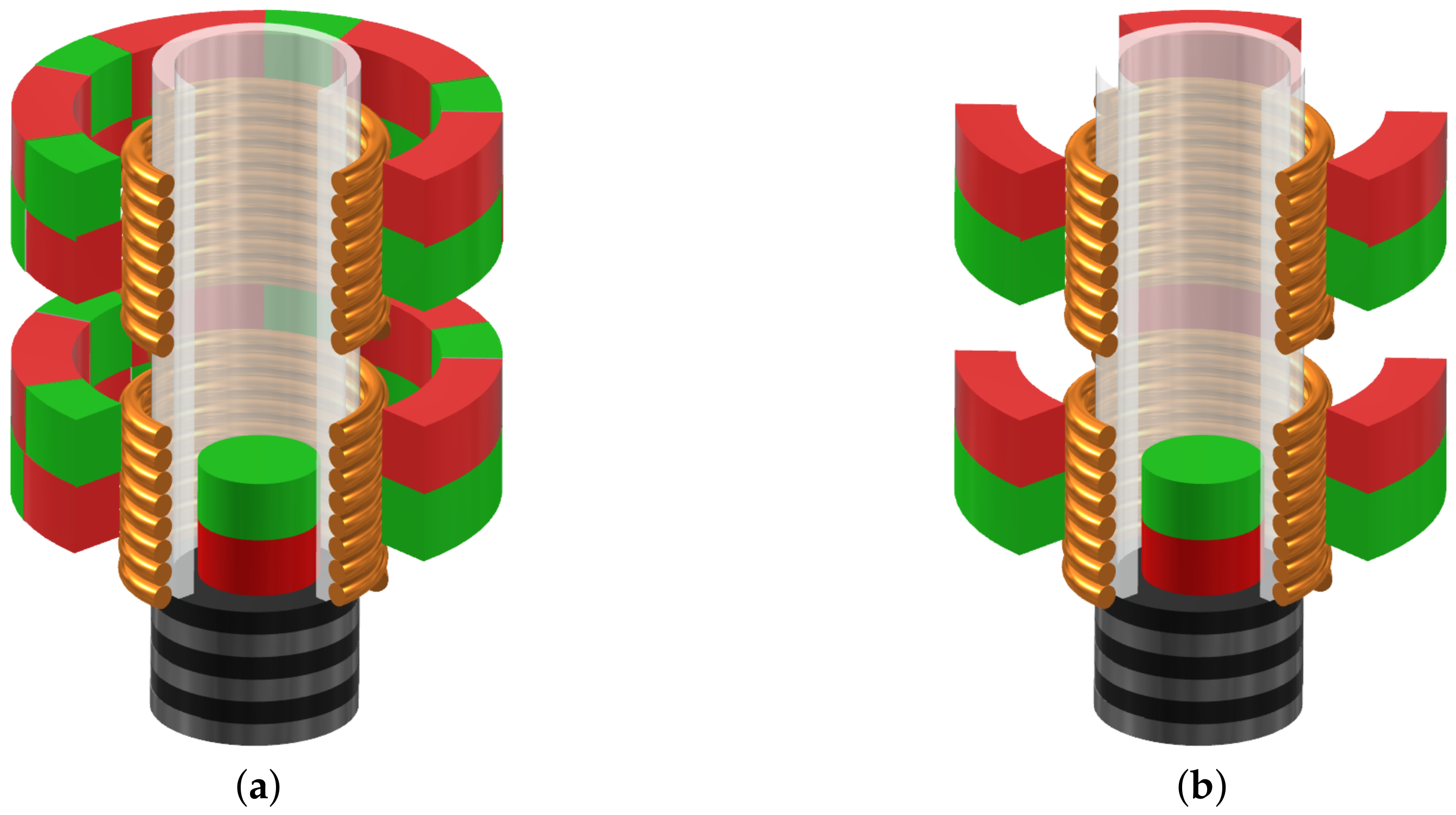
3.1. Multistability Consideration

The property of a magnet to either attract or oppose another magnet can be used to generate stable equilibrium positions, as far as the moving magnet is constrained to a single DoF motion, as is enforced by the glass tube in our case. An equilibrium position results from the overall force acting on the proof mass, being equal to zero. For a vertical setup, this corresponds to the intersection of the magnetic force with the absolute value of the gravitational force of the proof mass. Moreover, this resting position is stable if the force gradient at this point is negative, i.e., a slight deviation of the proof mass to a higher position leads to a negative force and vice versa. The stability can be proved by Lyapunov’s direct method [34]. Provided that the maximum magnetic force is larger than the gravitational force, there exists at least a single stable equilibrium position. In our previous work [15], a second stable position was generated due to the contact with the stack actuator. Here, we take advantage of the nonlinearity of the magnetic force to generate a larger number of equilibria at predefined positions by superimposing magnetic fields of multiple ring magnets. For this purpose, we use a cylindrical proof mass with 1 mm height and diameter. The magnets’ dimensions used in this study are given in Table 1.
In general, the number of generated equilibria corresponds to the number of ring magnets used in the setup. Our goal is to imprint resting positions at integral multiples of 2.5 mm for a cylindrical permanent magnet with 1 mm height and diameter. For a design comprising two ring magnets (setup 1), the resulting magnetic force is visualized in Figure 4a. The underlying setup parameters are given in Table 2.
It is important to mention that the larger the ring magnets’ dimensions and magnetic remanences, the larger the minimum possible distance between the two equilibrium positions. This results from the fact that, otherwise, a ring magnet generating a stable equilibrium at one position simultaneously implies a force at the desired lower position that may be either too large or too negative to be canceled by the lower magnet. This makes a systematic search for a feasible design difficult; we were able to find only a few feasible solutions for Setup 1, using unusually small remanence values (see Table 2). Similar to our previous work [15], this problem can be mitigated by utilization of an additional magnet, which is not used to generate another equilibrium, but to weaken the field of the highest magnet. Thus, we could be more flexible by the choice of the magnetic remanences. Setup 2 in Figure 4b demonstrates the advantage of this approach. Here, the two predefined resting positions were achieved by using identical ring magnets with remanences of 0.2 T, which corresponds to the lowest possible value for hard ferrite and is therefore considered producible. For Setup 1, the design is not feasible for such remanence values.
It is possible to extend the presented actuator to more equilibrium positions by stacking a larger number of ring magnets. Two examples are shown: Figure 5a shows three equilibria generated by four ring magnets, and in Figure 5b, four resting positions are imprinted by five magnets.
We are not aware of a general limitation for the maximum number of equilibria that can be generated, but assume that it depends on the specific magnet parameters. It should be noted, however, that finding a suitable setup is not a trivial task and may not be achieved heuristically for larger setups. An optimization-based search may, therefore, be used to reduce this effort, but its solution strongly depends on a well-chosen a priori estimation of the individual magnet positions, which is generally difficult to achieve.
Moreover, the small size of the ring magnets can pose a challenge. We assume that similar results as those presented in this work can be obtained by generating weaker magnetic fields using different magnets, e.g., by replacing the small ring magnet by a larger one with internally alternating magnetizations, comparable to Halbach arrays [35], or an axis-symmetric distribution of smaller magnets. These alternative concepts are visualized in Figure 6 and should be investigated in further research. For the simulation results of the control approach in the following section, Setup 1 given in Table 2 is used.

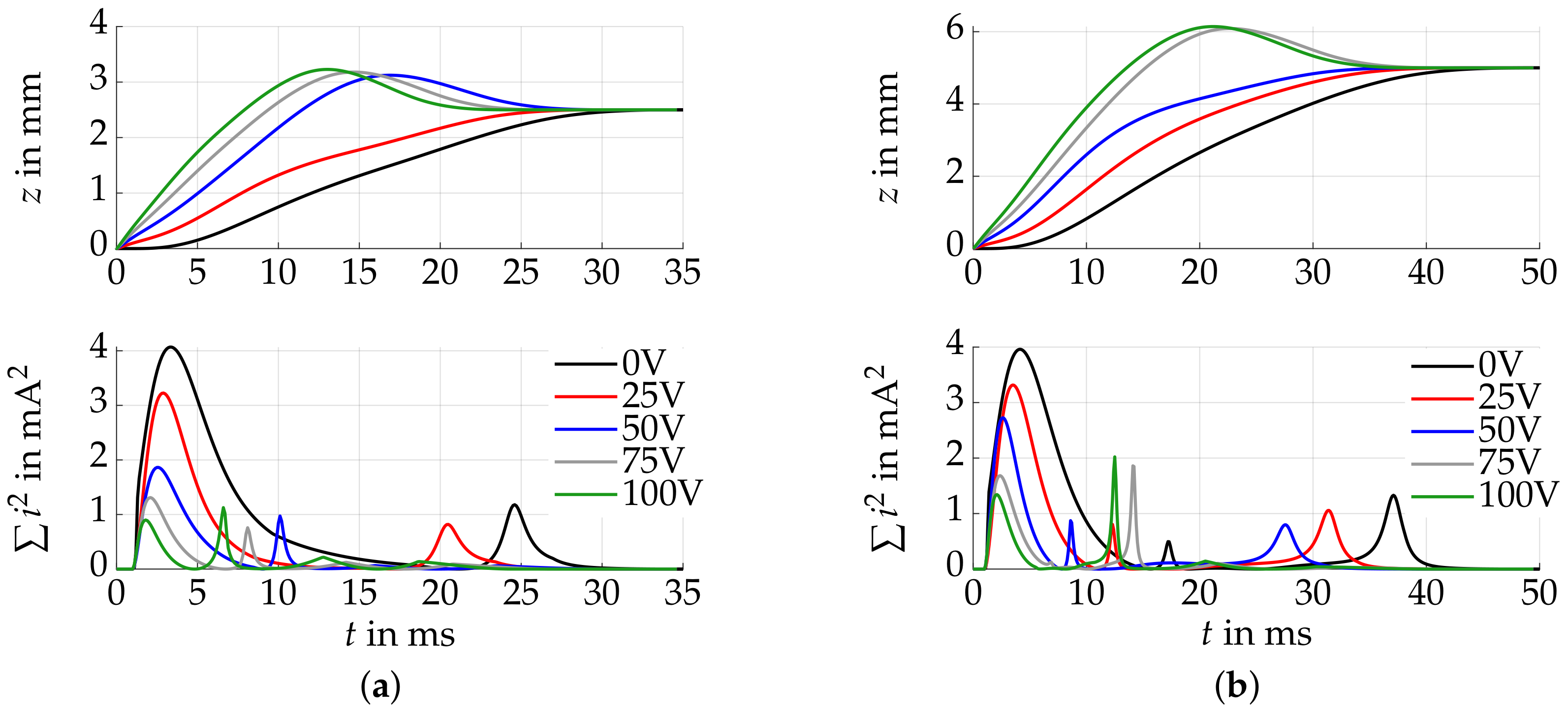
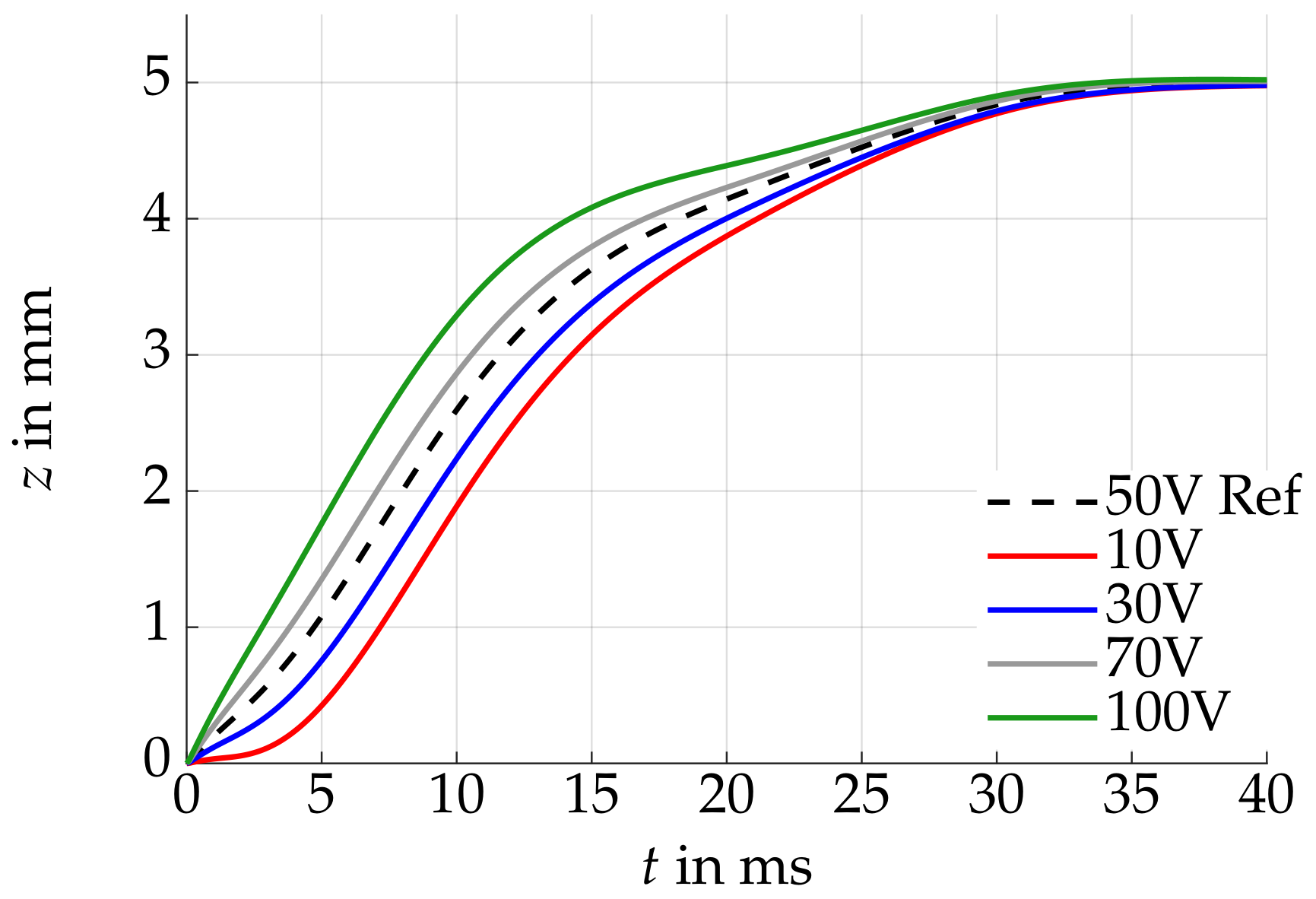
3.2. Simulation Study

Given the magnetic setup with two equilibrium positions (Setup 1), we now want to demonstrate the effectiveness of the cooperation between the kick and catch actuators as well as the control approach in simulation. The setup parameters are given in Table 3. The parameters concerning trajectory planning and control are summarized in Table 4, where the controller gain matrices K i , K z for the inner and outer control loop result from the chosen poles p i and p z . Note that, due to the strong dependency of the optimized trajectory from the initial velocity v 0 after the kick, it proves convenient that the parameters λ l of the superimposed trajectory (35) also depend on the velocity. In the remainder of this work, we use the heuristically chosen law as follows:
λ = [ 6 , 8 , 10 ] + 2.5 v 0 ,
which seems sufficient for this study. However, a more general expression may be derived by a preceding optimization, which is out of the scope of this work.
Starting with the proof mass located on top of the stack actuator, we initiate the kick using different voltages between 0 V (no kick) and 100 V (full kick). Recall that the goal is to reduce the solenoid currents. Therefore, all motions are optimized with respect to the cost function (28). In the following, we use four parameters σ s , s = 1 , , 4 to describe the trajectory. The simulations are carried out for the transition of the proof mass to both the middle and upper equilibria; the results are visualized in Figure 7.
It can be seen that the piezoelectric kick has a positive effect on the efficiency by largely reducing the input currents and simultaneously achieving faster transitions to both resting positions. Between the missing and full kick, the sum of squared currents is reduced by 87% for the transition to the lower resting position and by 82% for the motion to the upper equilibrium. Simultaneously, the transient time can be reduced by up to 32% and 11%, respectively. This result confirms the assumption of our previous work [15], where only a single piezo voltage and equilibrium position were used to demonstrate this effect. In the time course of the squared currents in Figure 7b, a second peak in the current can be seen for each kick. This corresponds to the current needed to decelerate the proof mass. This suggests that for larger piezo forces, the kick may have the opposite effect, due to an increased effort for damping the magnet velocity. For a general setup, the kick should therefore, be optimized simultaneously with the trajectory.
So far, we assumed that for a certain voltage, each kick is identical and corresponds to the time course predicted by our model, which in turn allows us to precisely follow the trajectory. However, the preliminary experiments showed that this is not necessarily the case, e.g., due to random impact between the proof mass and the guiding tube. This results in an unexpected initial state when the controller is switched on after the kick. In order to compensate for such disturbances, feedback control is used. Here, we approximate the effect of an initial disturbance by applying a different voltage to the piezo than what was expected within the optimization. The ability to asymptotically converge to the intended motion is demonstrated, using the 50 V -kick to the upper equilibrium. The initial state uncertainty is artificially generated by both higher and lower voltage impulses. In all simulated cases, the controller is able to compensate the disturbance within the transition time as seen in Figure 8.
Finally, we evaluate the efficiency of the trajectory generator in terms of minimum energy effort. To this end, we compute reference motions using a different number of optimization parameters σ s . The trajectories are then compared with the costs of the classical unoptimized approach, i.e., connecting multiple polynomials. As mentioned in Section 2.2.3, the polynomials tend toward large overshoots when combined with the piezoelectric kick. Thus, we neglect the kick and only apply electromagnetic actuation for the following comparison. We evaluate the overall costs of a motion containing all combinations of transitions between the three equilibrium positions. A visualization of the costs over the number of optimization parameters is given in Figure 9. Three of these trajectories are shown in Figure 10, namely, the unoptimized polynomial trajectory and two optimized ones with 2 and 20 optimization parameters σ s .
Although the polynomial trajectory is the smoothest one, the optimized motions are more efficient, compared to the cost function. As was expected, the cost function values decrease with the increasing number of parameters. However, the optimized solution using a single parameter σ s is less efficient than the time-optimized polynomial trajectory. This is due to the fact that the σ -dependent trajectory uses an exponential function for transitions from the bottom to an upper equilibrium, which is less effective than the polynomial in the case where there is no piezoelectric kick. For s > 1 , the superposition strategy is more efficient than the polynomial trajectory. Moreover, the polynomial trajectory can result in a large overshoot when applied after the kick motion.
An interesting result corresponds to the non-smoothness of the optimized trajectories, which appears in the form of larger spikes in the electrical current. Compared to the mostly smooth input for the polynomial approach, the optimized trajectories make use of short but high current spikes in order to efficiently move the proof mass. Although the maximum input current is larger for the optimized trajectories, the evaluated time integral is smaller for the trajectory with 20 parameters, and the costs concerning the transition times are lower for both optimized trajectories. The correlation between the trajectory smoothness and the cost function should be investigated in the future. For a final assessment of the quality of the presented optimization approach, knowing the lower bound, i.e., the global minimum, is an advantage. This could be realized by a global optimizer, such as a genetic algorithm.
It should be mentioned that the nominal trajectory plays an important role for finding a meaningful solution, but may also prevent the optimization algorithm from finding a better optimum. Therefore, a considered choice should be made beforehand. Eventually, the individual motions could now be stored on the controller hardware of a real setup and run on command to initiate the respective motion. Due to its general simplicity, we assume that the presented approach can also be used as an initial solution for similar flat 1-DoF systems.

4. Discussion

The magnetic microactuator has several advantages, such as multiple, asymptotically stable equilibria and the expandability to a larger number of resting positions. This can prove useful for future applications, where large working ranges are necessary, and the proof mass is desired to remain in its position, even without a constant energy supply. We have shown that a cooperative mechanism combined with an optimal control strategy is useful for reducing the electrical load on the solenoids, which results in less heat loss and may extend the durability of the components. Moreover, the control strategy is generalizable to an arbitrarily extended design, such that the implementation effort is kept low. However, the non-smooth behavior of the optimized electrical currents may be undesirable in an experimental setup. Smoother motions can be obtained by specifying trajectories that are differentiable more often. In contrast to other stable actuator concepts, the transitions between the equilibrium positions are unstable and the controller design is indispensable. This means that for an experimental setup, sensors for measuring the solenoid currents and the proof mass position are necessary. The latter can be challenging, especially when cost-effective solutions are preferred. Therefore, principles based on induced voltage or measuring the magnetic field can be investigated.
Moreover, the proposed approach assumes fully known permanent magnetic fields without variability in their homogeinity and field strength, which is generally not the case for real magnets. While it may be possible to experimentally adapt the magnet positions to achieve multiple stable equilibria at predefined positions, such an uncertainty in the magnetic field is problematic for the proof mass motion, due to the strong model dependence of the inverse computation within the control algorithm. Although a rough estimation of the magnet tolerances for which the trajectories can be tracked with acceptable error could be achieved through extensive simulation, careful measuring of the single magnets may still be necessary before assembly. For this reason, we suggest a first estimation of appropriate magnets in simulation, experimentally identifying the corresponding real magnets, and subsequently recomputing the magnet positions and trajectories based on the obtained values. Since small changes in the magnetic field mostly affect the inverse computation of the solenoid voltages rather than the cascaded linear control loops, we assume that the choice of the controller gains can be adopted from the initial simulation without change.
Another important question concerns the possible miniaturization of such a microactuator, which is closely linked to further research on its general limitations. In this work, we showed that the magnets’ dimensions and remanences are strongly coupled with the realizability of multiple equilibrium positions, particularly when short distances between them are needed. Two possible solutions are, therefore, proposed: a Halbach array-like permanent magnet or multiple smaller magnets. In both cases, the resulting force curve should be large enough to generate a robust equilibrium, but narrow in terms of little impact on the neighboring resting positions. Extensive finite element modeling will, therefore, be necessary. Finally, the efficiency of the overall system can further be improved by simultaneously optimizing both the controller and the design, such that couplings between them are exploited. It also motivates the investigation of fast, nonlinear optimal control methods, which can enrich both control theory and microactuator technology.

5. Conclusions

In this work, we presented the extension of a cooperative, magnetic microactuator by multiple, asymptotically stable equilibrium positions. This was achieved by shaping the magnetic field by several ring magnets. Additional solenoids were used to allow motions of a magnetic proof mass over a large working range. It was shown that, in general, the setup is expandable to multiple, asymptotically stable equilibria at predefined positions. For the realization of the underlying magnetic fields, two alternatives, besides small ring magnets, were proposed to be investigated in future work. Moreover, we presented a control strategy that ensures efficient switching of the proof mass between the resting positions. This approach was designed in such a way that it is generalizable to an arbitrary number of solenoids and minimizes the input current needed by the proof mass to follow a given reference trajectory. This was also supported by an optimal trajectory planning approach that considers a cooperative interaction between a piezoelectric stack actuator and the solenoids. We assume that the actuator principle and control approach are beneficial for both the microactuator and control engineering community. However, the presented model corresponds to an approximation and may be limited to hard magnetic materials with small mutual influence on the respective magnetization. Moreover, the model parameters are critical for an accurate compliance with the actual setup. It is, therefore, important to adapt the model to the measured data. For this purpose, the presented theory will be verified based on an experimental system in future work, upon which further investigations of the limitations of the approach can be carried out.

Author Contributions

Conceptualization, C.A. and T.B.; funding acquisition, C.A. and T.B.; methodology, M.O.; software, M.O.; investigation, M.O. and A.S.; writing—original draft preparation, M.O.; visualization, M.O.; supervision, C.A. and T.B. All authors have read and agreed to the published version of the manuscript.

Funding

This research was funded by the German Research Foundation (DFG) within the priority program SPP2206 “KOMMMA”, project “Kick and Catch-Cooperative Microactuators for Freely Moving Platforms”.

Conflicts of Interest

The authors declare no conflict of interest.

References

  1. Mita, M.; Arai, M.; Tensaka, S.; Kobayashi, D.; Fujita, H. A Micromachined Impact Microactuator Driven by Electrostatic Force. J. Microelectromech. Syst. 2003, 12, 37–41. [Google Scholar] [CrossRef]
  2. Min, H.J.; Lim, H.J.; Kim, S.H. A new impact actuator using linear momentum exchange of inertia mass. J. Med. Eng. Technol. 2002, 26, 265–269. [Google Scholar] [CrossRef]
  3. Peng, Y.; Liu, L.; Zhang, Y.; Cao, J.; Cheng, Y.; Wang, J. A smooth impact drive mechanism actuation method for flapping wing mechanism of bio-inspired micro air vehicles. Microsyst. Technol. 2018, 24, 935–941. [Google Scholar] [CrossRef]
  4. Huang, W.; Sun, M. Design, Analysis, and Experiment on a Novel Stick-Slip Piezoelectric Actuator with a Lever Mechanism. Micromachines 2019, 10, 863. [Google Scholar] [CrossRef] [PubMed] [Green Version]
  5. Breguet, J.M.; Pérez, R.; Bergander, A.; Schmitt, C.; Clavel, R.; Bleuler, H. Piezoactuators for Motion Control from Centimeter to Nanometer. In Proceedings of the IEEE/RSJ International Conference on Intelligent Robots and Systems, Takamatsu, Japan, 31 October–5 November 2000; pp. 492–497. [Google Scholar]
  6. Hernando-García, J.; García-Caraballo, J.L.; Ruiz-Díez, V.; Sánchez-Rojas, J.L. Motion of a Legged Bidirectional Miniature Piezoelectric Robot Based on Traveling Wave Generation. Micromachines 2020, 11, 321. [Google Scholar] [CrossRef] [PubMed] [Green Version]
  7. Ruiz-Díez, V.; Hernando-García, J.; Sánchez-Rojas, J.L. Linear motors based on piezoelectric MEMS. Proceedings 2020, 64, 9. [Google Scholar] [CrossRef]
  8. Floyd, S.; Pawashe, C.; Sitti, M. An Untethered Magnetically Actuated Micro-Robot Capable of Motion on Arbitrary Surfaces. In Proceedings of the IEEE International Conference on Robotics and Automation, Pasadena, CA, USA, 19–23 May 2008; pp. 419–424. [Google Scholar] [CrossRef]
  9. Dieppedale, C.; Desloges, B.; Rostaing, H.; Delamare, J.; Cugat, O.; Meunier-Carus, J. Magnetic bistable micro-actuator with integrated permanent magnets. In Proceedings of the IEEE Sensors, Vienna, Austria, 24–27 October 2004; pp. 493–496. [Google Scholar] [CrossRef]
  10. Stepanek, J.; Rostaing, H.; Lesecq, S.; Delamare, J.; Cugat, O. Position Control of a Levitating Magnetic Actuator Applications to Microsystems. In Proceedings of the 16th Triennial World Congress, Prague, Czech Rebublic, 4–8 July 2005; pp. 85–90. [Google Scholar] [CrossRef] [Green Version]
  11. Ruffert, C.; Gehrking, R.; Ponick, B.; Gatzen, H.H. Magnetic Levitation Assisted Guide for a Linear Micro-Actuator. IEEE Trans. Magn. 2006, 42, 3785–3787. [Google Scholar] [CrossRef]
  12. Ruffert, C.; Li, J.; Denkena, B.; Gatzen, H.H. Development and Evaluation of an Active Magnetic Guide for Microsystems With an Integrated Air Gap Measurement System. IEEE Trans. Magn. 2007, 43, 2716–2718. [Google Scholar] [CrossRef]
  13. Laurent, G.J.; Delettre, A.; Zeggart, R.; Yahiaoui, R.; Manceau, J.F.; Le Fort-Piat, N. Micropositioning and Fasst Transport Using a Contactless Micro-Conveyor. Micromachines 2014, 5, 66–80. [Google Scholar] [CrossRef] [Green Version]
  14. Poletkin, K.; Lu, Z.; Wallrabe, U.; Korvink, J.G.; Badilita, V. Stable dynamics of micro-machined inductive contactless suspensions. Int. J. Mech. Sci. 2017, 131, 753–766. [Google Scholar] [CrossRef] [Green Version]
  15. Olbrich, M.; Schütz, A.; Kanjilal, K.; Bechtold, T.; Wallrabe, U.; Ament, C. Co-Design and Control of a Magnetic Microactuator for Freely Moving Platforms. Proceedings 2020, 64, 23. [Google Scholar] [CrossRef]
  16. Schütz, A.; Hu, S.; Rudnyi, E.B.; Bechtold, T. Electromagnetic System-Level Model of Novel Free Flight Microactuator. In Proceedings of the 21st International Conference on Thermal, Mechanical and Multi-Physics Simulation and Experiments in Microelectronics and Microsystems, Cracow, Poland, 5–8 July 2020; pp. 1–6. [Google Scholar] [CrossRef]
  17. Schütz, A.; Olbrich, M.; Hu, S.; Ament, C.; Bechtold, T. Parametric system-level models for position-control of novel electromagnetic free flight microactuator. Microelectron. Reliab. 2021, 119, 1–9. [Google Scholar] [CrossRef]
  18. Goldfarb, M.; Celanovic, N. A lumped parameter electromechanical model for describing the nonlinear behavior of piezoelectric actuators. J. Dyn. Sys. Meas. Control 1997, 119, 478–485. [Google Scholar] [CrossRef]
  19. Gomis-Bellmunt, O.; Ikhouane, F.; Castell-Vilanova, P.; Bergas-Jane, J. Modeling and validation of a piezoelectric actuator. Electr. Eng. 2007, 89, 629–638. [Google Scholar] [CrossRef]
  20. Richter, H.; Misawa, E.A.; Lucca, D.A.; Lu, H. Modeling nonlinear behavior in a piezoelectric actuator. Precis. Eng. 2001, 25, 128–137. [Google Scholar] [CrossRef] [Green Version]
  21. Main, J.A.; Garcia, E. Piezoelectric Stack Actuators and Control System Design: Strategies and Pitfalls. J. Guid. Control Dynam. 1997, 20, 478–485. [Google Scholar] [CrossRef]
  22. Agashe, J.S.; Arnold, D.P. A study of scaling and geometry effects on the forces between cuboidal and cylindrical magnets using analytical force solutions. J. Phys. D Appl. Phys. 2008, 41, 1–9. [Google Scholar] [CrossRef]
  23. Ravaud, R.; Lemarquand, G.; Babic, S.; Lemarquand, V.; Akyel, C. Cylindrical Magnets and Coils: Fields, Forces, and Inductances. IEEE Trans. Magn. 2010, 46, 3585–3590. [Google Scholar] [CrossRef]
  24. Ansys Inc. ANSYS Electronics Desktop, Release 2020 R1; Ansys Inc.: Washington County, PA, USA, 2020. [Google Scholar]
  25. Specker, T.; Buchholz, M.; Dietmayer, K. Dynamical Modeling of Constraints with Friction in Mechanical Systems. In Proceedings of the 8th Vienna International Conference on Mathematical Modelling, Vienna, Austria, 18–20 February 2015; pp. 514–519. [Google Scholar]
  26. Fliess, M.; Lévine, J.; Martin, P.; Rouchon, P. Flatness and defect of non-linear systems: Introductory theory and examples. Int. J. Control 1995, 61, 1327–1361. [Google Scholar] [CrossRef] [Green Version]
  27. Mackenroth, U. Basic Properties of Multivariable Feedback Systems. In Robust Control Systems: Theory and Case Studies, 1st ed.; Springer: Berlin/Heidelberg, Germany, 2004. [Google Scholar]
  28. Charlet, B.; Lévine, J. On dynamic feedback linearization. Syst. Control Lett. 1989, 13, 143–151. [Google Scholar] [CrossRef]
  29. Bergman, K.; Ljungqvist, O.; Linder, J.; Axehill, D. An Optimization-Based Motion Planner for Autonomous Maneuvering of Marine Vessels in Complex Environments. In Proceedings of the 59th IEEE Conference on Decision and Control, Jeju Island, Korea, 14–18 December 2020; pp. 5283–5290. [Google Scholar] [CrossRef]
  30. Wu, Y.; Wang, H.; Zhang, B.; Du, K.L. Using Radial Basis Function Networks for Function Approximation and Classification. ISRN Appl. Math. 2012, 2012, 1–34. [Google Scholar] [CrossRef] [Green Version]
  31. The MathWorks Inc. MATLAB (R2019a); The MathWorks Inc.: Natick, MA, USA, 2019. [Google Scholar]
  32. Andersson, J. A General-Purpose Software Framework for Dynamic Optimization. Ph.D. Thesis, Department of Electrical Engineering (ESAT/SCD) and Optimization in Engineering Center, Heverlee, Belgium, October 2013. [Google Scholar]
  33. Wächter, A.; Biegler, L.T. On the implementation of a primal-dual interior point filter line search algorithm for large-scale nonlinear programming. Math. Program. 2006, 106, 25–57. [Google Scholar] [CrossRef]
  34. Khalil, H.K. Nonlinear Systems, 3rd ed.; Prentice Hall: Upper Saddle River, NJ, USA, 1996. [Google Scholar]
  35. Halbach, K. Design of permanent multipole magnets with oriented rare Earth cobalt material. Nucl. Instrum. Methods 1980, 169, 1–10. [Google Scholar] [CrossRef] [Green Version]
Figure 1. The multistable microactuator consists of a movable, cylindrical magnet within a guiding glass tube, a piezoelectric stack actuator (kick actuator), permanent magnets and electromagnets (catch actuators). The transparent part depicts a possible extension to a third levitating equilibrium.
Actuators 10 00183 g001
Figure 2. Combination of cascade control and flatness-based control. The linear partial system, i.e., the solenoids, are controlled by linear state feedback with controller gain matrix K i and prefilter S i (a) and the nonlinear system is handled using a feedback linearization approach (b). A trajectory generator is used to compute optimal reference motions and deviations between the current state and reference are compensated by a second linear controller with controller gain K z (c).
Actuators 10 00183 g002
Figure 3. Superimposed proof mass trajectory that fulfills the initial and final condition up to the second order. A nominal trajectory (blue) and an optimized, piecewise constant function (red) are superimposed and result in an optimal trajectory (black). The amplitudes of the piecewise function correspond to the optimization variables σ .
Actuators 10 00183 g003
Figure 4. Simulated magnetic force characteristic F pm of the superimposed magnetic fields. The intersections with the gravitational force (dashed, gray) correspond to the predefined, stable equilibria and are marked by red circles. (a) Setup 1: two equilibria are generated by superimposing two magnetic fields. (b) Setup 2: the identical resting positions are achieved by three ring magnets, but the choice of magnet parameters is more flexible. The third equilibrium of Setup 2, which is above 7 mm, is unintended and therefore not shown.
Actuators 10 00183 g004
Figure 5. Magnetic force characteristic for the extended, multistable microactuator. (a) Setup 3: Three stable equilibria (red circles) were generated by four ring magnets. (b) Setup 4: Four resting positions could be achieved with five ring magnets.
Actuators 10 00183 g005
Figure 6. Alternative concepts for achieving suitable magnetic force characteristics.(a) A Halbach array-like magnet design may be used to weaken the magnetic field. (b) Multiple single magnets can be used instead of a small ring magnet.
Actuators 10 00183 g006
Figure 7. Combined kick and catch trajectories to both equilibria for different piezoelectric kick voltages between 0 V and 100 V . Top panel: position z of the proof mass. Bottom panel: the respective sum of squared electrical currents. (a) The kick to the equilibrium at 2.5 mm is shown. (b) A similar effect is achieved for the kick to the equilibrium at 5 mm. In both cases, the electrical currents are reduced with increasing kick impact.
Actuators 10 00183 g007
Figure 8. Feedback control simulation compensating for initial state uncertainty. The expected initial state resulting in the reference trajectory (dashed, black) for 50 V is not achieved due to incorrect kick voltages. Feedback control compensates this error and the proof mass motion asymptotically converges to the desired trajectory for different piezo voltages.
Actuators 10 00183 g008
Figure 9. The trajectory costs over the number of parameters are shown. The red circle corresponds to the polynomial trajectory and the blue circles to the optimized motions. Although there is a fast cost function decrease for a low number of parameters, the costs oscillate and slightly increase for more than 10 optimization variables.
Actuators 10 00183 g009
Figure 10. Comparison of trajectories and respective currents with different numbers of optimization variables. (a) Top panel: for the polynomial trajectory, smooth motions were generated and the transition times were optimized. Middle panel: the trajectory with two parameters σ s and optimized transient time is less smooth but has lower costs. Bottom panel: the lowest costs were achieved with 20 parameters σ s . The dashed line corresponds to the desired final position of the proof mass. (b) The sum of squared currents corresponding to the different trajectories is shown. For the trajectory with 20 parameters, the solution is non-smooth due to fast changes in the current, but the transient time and the sum of squared currents are the lowest.
Actuators 10 00183 g010
Table 1. Magnet dimensions used in this study.
ComponentHeight in mmInner Radius in mmOuter Radius in mmMass in mg
Proof mass1 0.5 3.77
Ring magnet 0.5 1.5 2.2
Table 2. Experimental Setups 1–4 and respective parameters used to generate multiple equilibrium positions.
SetupMagnetRemanence in TPosition in mm
1 B r , p 0.1
B r , pm , 1 0.121.592
B r , pm , 2 0.13.296
2 B r , p 0.2
B r , pm , 1 0.21.225
B r , pm , 2 0.23.746
B r , pm , 3 0.26.338
3 B r , p 0.2
B r , pm , 1 0.21.143
B r , pm , 2 0.23.807
B r , pm , 3 0.26.223
B r , pm , 3 0.28.868
4 B r , p 0.2
B r , pm , 1 0.21.283
B r , pm , 2 0.23.670
B r , pm , 3 0.26.344
B r , pm , 4 0.28.701
B r , pm , 5 0.211.42
Table 3. Fixed design parameters that are used in the simulation.
DescriptionValueDescriptionValue
Inner radius (solenoid)0.8 mmResistance (solenoid)281 Ω
Outer radius (solenoid)1.2 mm F max (piezo)360 N
Height (solenoid)1.5 mm U max (piezo)100 V
Wire diameter (solenoid)25 μm k A (piezo)1.1 MNm−1
Specific resistance (solenoid)18 nΩmM (piezo)1.8 g
Number of turns (solenoid)1222 c A (piezo)25
Inductance (solenoid)3.9 mH f (proof mass)2.5 × 10⁻⁴
Mutual inductance (solenoid)2.0 mH k c (contact)4.5 × 10⁶
Position (solenoid 1)2.2 mm F (contact) m g
Position (solenoid 2)4.7 mm r d (contact)3
Table 4. Trajectory planning and control parameters used in simulation.
DescriptionValue
p i [ 400 + 100 i , 400 100 i ]
p z [ 200 + 100 i , 200 100 i , 150 ]
K i [ 280.3 , 1.19 ; 0.41 , 279.8 ]
K z [ 7500 , 110 , 0.5 ] × 10 3
T kick 1 ms
β 1
Publisher’s Note: MDPI stays neutral with regard to jurisdictional claims in published maps and institutional affiliations.

