Article

Robust Control of a Class of Nonlinear Discrete-Time Systems: Design and Experimental Results on a Real-Time Emulator

1
Laboratoire d’Informatique & Télécommunications, ECAM Rennes-Louis de Broglie, Campus de Ker Lann-Bruz, 35091 Rennes, France
2
Centre de Recherche en Automatique de Nancy, CRAN UMR 7039 CNRS, University of Lorraine, 54400 Cosnes-et-Romain, France
3
MACS Laboratory, National Engineering School of Gabes (ENIG), University of Gabes, Gabes 6029, Tunisia
4
IMS Laboratory, CNRS UMR 5218, Bordeaux INP, University of Bordeaux, 33405 Talence, France
*
Author to whom correspondence should be addressed.
Actuators 2021, 10(11), 303; https://doi.org/10.3390/act10110303
Submission received: 17 September 2021 / Revised: 6 November 2021 / Accepted: 9 November 2021 / Published: 18 November 2021

Abstract

:
The aim of this study is to develop a new observer-based stabilization strategy for a class of Lipschitz uncertain systems. This new strategy improves the performances of existing methods and ensures better convergence conditions. Sliding window approach involves previous estimated states and measurements in the observer and the control law structures which increase the number of decision variables in the constraint to be solved and offers less restrictive Linear Matrix Inequality (LMI) conditions. The established sufficient stability conditions are in the form of Bilinear Matrix Inequality (BMI) which is solved in two steps. First, by using a slack variable technique and an appropriate reformulation of the Young’s inequality. Second, by introducing a useful approach to transform the obtained constraint to a more suitable one easily tractable by standard software algorithms. A comparison with the standard case is provided to show the superiority of the proposed H observer-based controller which offers greater degree of freedom. The accuracy and the potential of the proposed process are shown through real time implementation of the one-link flexible joint robot to ARDUINO UNO R3 device and numerical comparison with some existing results.

1. Introduction

1.1. Background

In many industrial processes, developing a perfect model to the system dynamics is crucial either to build a controller or to obtain real time information on the system for surveillance. Sometimes, data errors, disconcerted parameters, environmental noise, disturbances or even the age of the system can lead to modeling errors. These errors can cause a deviation of the dynamics during surveillance or decision-making. In fact, the presence of uncertainties leads to instability, divergence or degraded controller performance. Therefore, robust uncertainty stabilization methods have been proposed to filter disturbances and uncertainties and ensure a good degree of noise sensitivity, good performance and robustness. Many remarkable methods have been synthesized: robust stabilization via output feedback [1,2], H control for systems with uncertain parameters [3,4] and Lipschitz nonlinearities [5], finite-time control for one-sided Lipschitz nonlinear systems [6], interval observers for global feedback control [7], feedback Stabilization with nonlinear output [8] and adaptive sliding mode control with finite-time [9] and tracking problem [10].
The dynamic behavior of a process can be fully described by the evolution of its state variables. Thus, many industrial systems require the measurement of several physical variables in order to guarantee supervision or control while ensuring a minimum level of performance [11,12]. However, it is very difficult, if not impossible, to measure all these variables mainly for cost and/or technical reasons. A usual way of addressing this problem is to place software sensors, or observers, which construct a reliable estimation to the whole system dynamics from the available information on inputs, outputs and the dynamic model of the process [13,14,15]. Observer design is part of estimation theory with applications, practically, to all fields of engineering, as evidenced by the large number of published works in this field [16,17]. Furthermore, many researchers focus on the observer-based controller design for nonlinear continuous or discrete-time systems. Interesting results are presented in [5,18,19]. In [18], for example, a two steps methodology for computing the observer and controller gains for Lipschitz systems is presented in the form of LMI conditions. In [19], a unique optimization problem, based on the diagonal Lyapunov matrix, is necessary to calculate both the observer gain and the controller gain. Recently, an interesting publication of [5] presents a useful scheme consisting on the use of a symmetric Lyapunov function to design robust observer-based stabilization for nonlinear systems. A slack variable technique inspired from [20] and the Young’s inequality allow to handle the difficulty of Non-deterministic Polynomial-time hard (NP-hard) nature of the problem. All these interesting results use only the last available state and measurement to synthesis the observer/controller gains.
This work is motivated by recent results on observer design [21,22], and the idea here is to synthesize a new observer-based control methodology for a class of Lipschitz discrete-time systems in the presence of bounded disturbances and parametric uncertainties. By simply using a sliding window of measurements in a Luenberger observer and a sliding window of delayed states in the controller, additional decisions variables can be introduced and thus the optimization problem is strengthened. Contrary to conventional approaches that consider only the last available measurement for the observer and the last available state estimate for the controller [5], adding a defined number of previous states and measurements in the observer and controller structures improves the disturbance rejection and allows promoting the robustness of the designed observer-based control. In order to add more degree of freedom in the optimization problem and obtain less conservative LMI conditions, a slack variable technique [20] with a reformulation of the Young’s inequality [23] are used. In order to highlight the contribution proposed in this paper, the improvements are summarized as follows with respect to existing results:
  • The problem of using previous measurements in the observer structure and estimated states in the control law, in presence of modeling uncertainties, has not been tackled before. For example, the Kalman filter uses the previous measurements with a single regression step ( r = 1 ) but what is proposed in this paper is to solve an estimation-control problem in dual form (a single resolution step from LMI) with sliding windows of estimated states and measurements ( r > 1 ).
  • The sliding window approach allows to introduce additional decision variables to the convex problem which add more degree of freedom.
  • The proposed linear constraint allows to compute the controller and the observation gains in dual form (only one resolution step) contrary to the approaches in [18,20,24].
  • A more optimal use and introduction of Young’s inequality will be proposed other than the classical ones [5]. This will increase the degree of freedom when synthesizing a robust control law as well as the treatment of less conservative LMIs.
  • A technique for handling and transforming BMI constraints into LMI is used. This technique is based on the inclusion of a “Slack-Variable”. This subsequently makes it possible to eliminate the difficulty of calculating or optimizing bilinear terms.
The outline of the paper is organized as follows. Some useful notations and preliminaries are presented in the next part of this section. Section 2 introduces the problem formulation. In Section 3, the synthesis procedure of the robust sliding window observer-based controller is detailed and a particular solution is proposed to overcome the problem of BMI. Section 4 presents a comparison with the standard case and a discussion on the enhancement of the main approach of this paper is given. In Section 5, experimental results are provided. They confirm the high quality of stabilization offered by the proposed approach through a real-time implementation based on ARDUINO UNO R3 board that is used as an Digital Signal Processing (DSP) emulator through target mode (Hardware In the Loop). Finally, concluding remarks can be found in Section 6.

1.2. Notation

The following notation will be used throughout this paper:
  • In a matrix, the notation ( ) represents the blocks induced by symmetry.
  • e p ( i ) represents a vector of the canonical basis of R p , where
    e p ( i ) = 0 , , 0 , 1 , 0 , , 0 i th p components T R p , p 1 .
  • Z = Z T Z is the Euclidean vector norm.
  • Z T is the transposed matrix of Z.
  • I p represents the identity matrix of dimension p.
  • Z is a square matrix. The notation Z > 0 ( Z < 0 ) means that Z is positive definite (negative definite).
  • The l 2 norm of the vector Z R p is given by Z l 2 p and is defined as Z l 2 p = k = 0 Z k 2 .

1.3. Preliminaries

Lemma 1
([23]).Consider a nonlinear function g : R n R n , the following two items are equivalent:
  • g is globally Lipschitz with respect to its argument, i.e.,
    g ( a ) g ( b ) γ g a b , a , b R n .
  • there exist constants g i j ̲ and g i j ¯ so that for all     a , b R n there exist z i C o ( a , b ) , z i a , z i b and functions g i j : R n × R n R satisfying the following equality:
    g ( a ) g ( b ) = i , j = 1 q , n g i j ( z i ) H i j ( a b )
    and g i j ̲ g i j ( z i ) g i j ¯ where g i j ( z i ) = g i x j ( z i ) and H i j = e q ( i ) e n T ( j ) .
Lemma 2
([23]).Let X and Y be two matrices of appropriate dimensions. For any symmetric positive definite matrix S of appropriate dimension, the following variant of Young’s relation holds:
X T Y + Y T X 1 2 X + S Y T S 1 X + S Y
It can be seen that only half of X T Y + Y T X is majored. This result adds more degree of freedom and provides a more general and relaxed LMI conditions as detailed in [23].
Lemma 3
([25]).Consider three matrices X, Y and S of appropriate dimensions with S T S I . Then, η > 0 , the following inequality holds:
X S Y + Y T S T X T η X X T + 1 η Y T Y

2. Problem Formulation

Consider the following class of nonlinear uncertain systems:
x ( k + 1 ) = A + Δ A ( k ) x ( k ) + B u ( k ) + D g x ( k ) + E 1 ω ( k ) y ( k ) = C + Δ C ( k ) x ( k ) + E 2 ω ( k )
where x ( k ) R n , u ( k ) R m , y ( k ) R p and ω ( k ) R s are the state, the input, the output and the disturbance vectors, respectively. A R n × n , B R n × m , C R p × n , D R n × p , E 1 R n × s and E 2 R p × s are constant matrices. g : R n R q is a Lipschitz nonlinear vector. Δ A ( k ) and Δ C ( k ) are unknown matrices representing time-varying parameter uncertainties with
Δ A ( k ) = M 1 F ( k ) N 1
Δ C ( k ) = M 2 F ( k ) N 2
where the unknown matrix F ( k ) satisfies the following condition:
F ( k ) T F ( k ) I .
For the system (5), we consider the following sliding measurement window observer:
x ^ ( k + 1 ) = A x ^ ( k ) + B u ( k ) + D g x ^ ( k ) + L y ( k ) C x ^ ( k ) y ( k 1 ) C x ^ ( k 1 ) y ( k r + 1 ) C x ^ ( k r + 1 )
where r, L and x ^ ( k ) represent, respectively, the number of the considered measurements, the global observer gain matrix and the state estimate.
To include the sliding window of measurements, Equation (5) can be rewritten until the following form:
z ( k + 1 ) = A + Δ A ( k ) z ( k ) + B u ( k ) + D g I T z ( k ) + E 1 ν ( k )
with
z ( k ) = x ( k ) x ( k 1 ) x ( k r + 1 ) , ν ( k ) = ω ( k ) ω ( k 1 ) ω ( k r + 1 ) , A = A 0 0 I n 0 0 0 0 0 I n 0 ,
Δ A ( k ) = Δ A ( k ) 0 0 0 0 0 0 0 0 = M 1 F ( k ) N 1 , M 1 = M 1 0 0 , N 1 = N 1 0 0 ,
B = B 0 0 , D = D 0 0 , I = I n 0 0   and   E 1 = E 1 0 0 0 0 0 0 0 0 .
The new reformulation of the sliding window observer (8) is as follows:
z ^ ( k + 1 ) = A z ^ ( k ) + B u ( k ) + D g I T z ^ ( k ) + I L C ζ ( k ) + I L Δ C ( k ) z ( k ) + I L E 2 ν ( k )
where
ζ ( k ) = z ( k ) z ^ ( k ) , L = L 1 L 2 L r ,
Δ C ( k ) = block - diag Δ C ( k ) , , Δ C ( k ) r times = M 2 F ( k ) N 2 ,
F ( k ) = block - diag F ( k ) , , F ( k r + 1 ) , M 2 = block - diag M 2 , , M 2 r times ,
C = block - diag C , , C r times , N 2 = block - diag N 2 , , N 2 r times   and   E 2 = block - diag E 2 , , E 2 r times .
The considered observer is coupled with the following state estimate feedback controller:
u ( k ) = i = 1 r K i x ^ ( k i + 1 )
The controller (11) can be rewritten as follows:
u ( k ) = K z ^ ( k ) , K = K 1 K 2 K r
The observer gain L and the control gain K are unknown matrices to be determined such that the closed-loop system is asymptotically stable and satisfies the H criterion.
Define ζ ( k ) = z ( k ) z ^ ( k ) , the error between z ( k ) and its estimate. The dynamic of the estimation error ζ ( k + 1 ) = z ( k + 1 ) z ^ ( k + 1 ) is given by
ζ ( k + 1 ) = Δ A ( k ) I L Δ C ( k ) z ( k ) + ( A I L C ) ζ ( k ) + D g I T z ( k ) g I T z ^ ( k ) + ( E 1 I L E 2 ) ν ( k ) .
Using Equations (12), the closed-loop system can be rewritten as follows:
z ( k + 1 ) = A + Δ A ( k ) + B K z ( k ) B K ζ ( k ) + D g I T z ( k ) + E 1 ν ( k )
Then, using the fact that g ( . ) is a Lipschitz vector and applying Lemma 1, we obtain
g I T z ( k ) = i , j = 1 q , n φ i j H i j I T z ( k )
g I T z ( k ) g I T z ^ k = i , j = 1 q , n ϕ i j H i j I T ζ k
with g ̲ i j φ i j g ¯ i j , g ̲ i j ϕ i j g ¯ i j and H i j = e q ( i ) e n T ( j ) .
Using Equations (13)–(15b), an augmented global system can be defined as follows:
z ˜ ( k + 1 ) = A ˜ + Ξ ( Θ ) z ˜ ( k ) + E ˜ ν ( k )
with E ˜ T = E 1 T ( E 1 I L E 2 ) T , z ˜ ( k ) = z ( k ) ζ ( k ) , A ˜ = A + Δ A ( k ) + B K B K Δ A ( k ) I L Δ C ( k ) A I L C and   Ξ ( Θ ) = block - diag D i , j = 1 q , n φ i j H i j I T , D i , j = 1 q , n ϕ i j H i j I T .
The parameter Θ belongs to the bounded convex set H q n for which the set of vertices is defined by
V H q n = { φ , ϕ R q × n and φ i j , ϕ i j { g ̲ i j , g ¯ i j } } .
In the rest of the paper, the following notations will be used: Ξ 1 ( Θ ) = i , j = 1 q , n φ i j H i j and Ξ 2 ( Θ ) = i , j = 1 q , n ϕ i j H i j .

3. New Sliding Window Observer-Based Controller Design Methodology

This section presents the synthesis of the proposed observer-based controller approach. New enhanced stability conditions are detailed.

3.1. Stability Analysis

The main result of this article is proposed in the following corollary. The presented result is in the form of BMI. The linearization and the transformation of this constraint into a convex problem is detailed in the next section.
Corollary 1.
For a disturbance attenuation level λ > 0 , the robust H observer-based controller design problem corresponding to the system (5), the observer (8) and the state feedback controller (11) is solvable if there exist positive scalars η 1 , η 2 and η 3 , and matrices P ^ 1 , P 2 , P ^ 3 , Q ^ 1 > 0 , Q 2 R n r × n r , L R n × p r and K R m × n r such that the following BMI is feasible:
min λ subject to Π 0 0 0 0 0 Q 2 M 1 Q 2 I L M 2 0 0 0 0 0 Q ^ 1 N 1 T Q ^ 1 N 1 T Q ^ 1 N 2 T 0 0 0 0 0 0 0 0 0 0 0 0 0 0 0 ( ) 1 η 2 I 0 0 0 0 ( ) 1 η 3 I 0 0 0 ( ) ( ) η 1 I 0 0 ( ) ( ) ( ) η 2 I 0 ( ) ( ) ( ) ( ) η 3 I < 0
with
Π = Π 11 P ^ 3 Π 13 0 E 1 B K Q ^ 1 T ( ) Π 22 0 Π 24 Π 25 0 ( ) ( ) P ^ 1 P ^ 3 0 0 ( ) ( ) ( ) Π 44 0 I n × r ( ) ( ) ( ) ( ) λ 2 r I s × r 0 ( ) ( ) ( ) ( ) ( ) 1 2 Q ^ 1 Π 11 = P ^ 1 Q ^ 1 Q ^ 1 T + η 1 M 1 M 1 T Π 13 = A + D Ξ 1 ( Θ ) I T + B K Q ^ 1 T Π 22 = P 2 Q 2 Q 2 T Π 24 = Q 2 A + D Ξ 2 ( Θ ) I T I L C Π 25 = Q 2 ( E 1 I L E 2 ) Π 44 = P 2 + I G T G I T Θ V H q n .
Proof. 
In order to ensure the asymptotic stability of the closed loop system by the proposed H observer-based controller, the observer gain L and the controller gain K must satisfy the following H criterion:
G x x ^ l 2 λ ω l 2
where G is a known matrix and λ > 0 is the disturbance attenuation level that will be minimized. Therefore, we must look for a Lyapunov function V ( k ) such that
Δ V ( k ) + z ˜ ( k ) T I ˜ G I ˜ T z ˜ ( k ) λ 2 r ν T ( k ) ν ( k ) < 0 .
with x ( k ) = I T z ( k ) , x ^ ( k ) = I T z ^ ( k ) , I ˜ = block - diag I , I and G = block - diag 0 , G T G .
Let us consider the following candidate Lyapunov function:
V ( k ) = z ˜ T ( k ) P z ˜ ( k )
where P = P T > 0 is the matrix of Lyapunov.
The choice of the structure of the Lyapunov P matrix is influenced by the difficulty of the problem to be solved. One of the most used structures to solve the problem of observer-based controller is P = block - diag P 1 , P 2 . This particular structure allows to simplify the calculation by eliminating some couplings between the observer and controller gains. However, the resulting LMI remains conservative. To improve the existing results, a non-diagonal Lyapunov matrix is used in this contribution in order to get a more relaxed LMI conditions. Then, we propose the following structure for the matrix P:
P = P 1 P 3 P 3 T P 2 .
Define Δ V ( k ) = V ( k + 1 ) V ( k ) . Then, the inequality (20) is equivalent to
z ˜ ( k ) ν ( k ) T A ˜ + Ξ ( Θ ) T P A ˜ + Ξ ( Θ ) P + I ˜ G I ˜ T A ˜ + Ξ ( Θ ) T P E ˜ ( ) E ˜ T P E ˜ λ 2 r I s × r z ˜ ( k ) ν ( k ) < 0 .
Note that the inequality (23) is satisfied if
A ˜ + Ξ ( Θ ) T P A ˜ + Ξ ( Θ ) P + I ˜ G I ˜ T A ˜ + Ξ ( Θ ) T P E ˜ ( ) E ˜ T P E ˜ λ 2 r I s × r < 0
which is equivalent, using Schur’s lemma, to
P 1 A ˜ + Ξ ( Θ ) E ˜ ( ) P + I ˜ G I ˜ T 0 ( ) ( ) λ 2 r I s × r < 0 .
The inequality (25) is still unresolved due to its bilinear nature caused by the existence of the unknown matrix P and its inverse P 1 . The next step consists to propose a new approach to overcome this major obstacle using an LMI approach based on a judicious use of Young’s reformulation. Thus, we obtain sufficient and less conservative conditions ensuring the stability of the closed-loop system.
As the variables P and P 1 are interdependent, they should not exist simultaneously in the same constraint. To eliminate the P 1 matrix, the idea is to introduce a slack variable Q of appropriate dimensions and to pre-multiply (25) by the matrix block - diag ( Q , I , I ) and post-multiply it by the block - diag ( Q T , I , I ) matrix. Then, using the inequality Q P 1 Q T T P Q Q T , the inequality (25) is then equivalent to
P Q Q T Q A ˜ + Ξ ( Θ ) Q E ˜ ( ) P + I ˜ G I ˜ T 0 ( ) ( ) λ 2 r I s × r < 0 .
Let us consider the following structure of the matrix Q:
Q = Q 1 Q 3 Q 4 Q 2 .
Using (22) and (27), the inequality (26) can be written as follows:
P 1 Q 1 Q 1 T P 2 Q 3 Q 4 T Π 13 Π 14 Q 1 E 1 + Q 3 ( E 1 I L E 2 ) ( ) P 2 Q 2 Q 2 T Π 23 Π 24 Q 4 E 1 + Q 2 ( E 1 I L E 2 ) ( ) ( ) P 1 P 3 0 ( ) ( ) ( ) P 2 + I G T G I T 0 ( ) ( ) ( ) ( ) λ 2 r I s × r < 0
with
Π 13 = Q 1 A + Δ A ( k ) + B K + D Ξ 1 ( Θ ) I T + Q 3 Δ A ( k ) I L Δ C ( k ) Π 14 = Q 1 B K + Q 3 A I L C + D Ξ 2 ( Θ ) I T Π 23 = Q 4 A + Δ A ( k ) + B K + D Ξ 1 ( Θ ) I T + Q 2 Δ A ( k ) I L Δ C ( k ) Π 24 = Q 4 B K + Q 2 A I L C + D Ξ 2 ( Θ ) I T .
Note here that while the gain L is coupled with Q 3 and Q 2 , the gain K is coupled with Q 1 and Q 4 . To overcome this problem, we can choose Q 3 = Q 4 = 0 . Then, we get the following structure of the matrix Q:
Q = block - diag Q 1 , Q 2 .
Through pre-multiplying and post-multiplying (28) by block - diag ( Q ^ 1 , I , Q ^ 1 , I , I ) and block - diag ( Q ^ 1 T , I , Q ^ 1 T , I , I ) with Q ^ 1 = Q 1 1 and using the notations P ^ 3 = Q ^ 1 P 3 , P ^ 1 = Q ^ 1 P 1 Q ^ 1 T , we get the following inequality:
P 1 Q 1 Q 1 T P ^ 3 Π 13 B K E 1 ( ) P 2 Q 2 Q 2 T Π 23 Π 24 Q 2 ( E 1 I L E 2 ) ( ) ( ) P ^ 1 P ^ 3 0 ( ) ( ) ( ) P 2 + I G T G I T 0 ( ) ( ) ( ) ( ) λ 2 r I s × r < 0
with Π 13 = A + Δ A ( k ) + B K + D Ξ 1 ( Θ ) I T Q ^ 1 T Π 23 = Q 2 ( Δ A ( k ) I L Δ C ( k ) ) Q ^ 1 T Π 24 = Q 2 A I L C + D Ξ 2 ( Θ ) I T . .
In inequality (30), we can notice that the matrix gain K is coupled with the matrix Q ^ 1 T in the term Π 13 , and not in Π 14 . Therefore, the idea consists in coupling the gain K , in Π 14 , with the matrix Q ^ 1 T . The inequality (30) can be written as follows:
P 1 Q 1 Q 1 T P ^ 3 Π 13 0 E 1 ( ) P 2 Q 2 Q 2 T Π 23 Π 24 Q 2 ( E 1 I L E 2 ) ( ) ( ) P ^ 1 P ^ 3 0 ( ) ( ) ( ) P 2 + I G T G I T 0 ( ) ( ) ( ) ( ) λ 2 r I s × r + 0 0 0 I n × r 0 X T ( B K ) T 0 0 0 0 Y + Y T X < 0 .
Researches usually use the standard young’s inequality to couple the controller gain with the Lyapunov matrix or the slack variable. In this contribution, we will use the reformulation of Young’s lemma [23]. In fact, this way to introduce the Young’s relation allows to have more degrees of freedom. Thus, by applying Lemma 2 on (31) with S = Q ^ 1 (in this case the matrix Q ^ 1 must be a symmetric positive matrix), the following inequality is obtained:
P ^ 1 Q ^ 1 Q ^ 1 T P ^ 3 Π 13 0 E 1 B K Q ^ 1 T ( ) P 2 Q 2 Q 2 T Π 23 Π 24 Q 2 ( E 1 I L E 2 ) 0 ( ) ( ) P ^ 1 P ^ 3 0 0 ( ) ( ) ( ) I G T G I T P 2 0 I n × r ( ) ( ) ( ) ( ) λ 2 r I s × r 0 ( ) ( ) ( ) ( ) ( ) 1 2 Q ^ 1 < 0
Using Lemma 3 and Equations (6), we obtain
P ^ 1 Q ^ 1 Q ^ 1 T P ^ 3 Π 13 0 E 1 B K Q ^ 1 T ( ) P 2 Q 2 Q 2 T 0 Π 24 Q 2 ( E 1 I L E 2 ) 0 ( ) ( ) P ^ 1 P ^ 3 0 0 ( ) ( ) ( ) I G T G I T P 2 0 I n × r ( ) ( ) ( ) ( ) λ 2 r I s × r 0 ( ) ( ) ( ) ( ) ( ) 1 2 Q ^ 1 + η 1 X 1 X 1 T + 1 η 1 Y 1 T Y 1 + η 2 X 2 X 2 T + 1 η 2 Y 1 T Y 1 + η 3 X 3 X 3 T + 1 η 3 Y 2 T Y 2 < 0
with
Π 13 = A + B K + D Ξ 1 ( Θ ) I T Q ^ 1 T X 1 = M 1 T 0 0 0 0 0 T X 2 = 0 M 1 T Q 2 T 0 0 0 0 T X 3 = 0 M 2 T L T I T Q 2 T 0 0 0 0 T Y 1 = 0 0 N 1 Q ^ 1 T 0 0 0 Y 2 = 0 0 N 2 Q ^ 1 T 0 0 0 .
Thus, by applying Schur’s lemma, we obtain the constraint (18). This ends the proof of Corollary 1. □

3.2. Converting BMI into LMI

To linearize the BMI given by (18), a change of variables for the terms coupled with the control gain K is defined:
K ^ = K Q ^ 1 T .
However, a simple change of variables cannot be applied for terms coupled with the observer’s gain L due to the presence of the matrix I . Therefore, a particular form of the matrix Q 2 is proposed to linearize the BMI (18):
Q 2 = Q 2 11 α 1 Q 2 11 α 1 Q 2 11 β 1 Q 2 11 Q 2 22 α 2 Q 2 22 α 2 Q 2 22 β 2 Q 2 22 α r 1 Q 2 r 1 , r 1 β 1 Q 2 11 β 2 Q 2 22 β r 1 Q 2 r 1 , r 1 Q 2 r r
with 0 α i < 1 and 0 β i < 1 for i { 1 , , r 1 } .
Thereafter, we can define the following changes of variables:
L ^ i = Q 2 11 L i , for i { 1 , , r }
Then, the BMI (18) is transformed into a convex problem.
After the resolution of the obtained LMIs problem, the observer and the controller gains can be computed through the following equations:
K = K ^ Q ^ 1 T
L i = ( Q 2 11 ) 1 L ^ i , for i { 1 , , r }
Remark 1.
The feasibility of the LMI procedure is raised when choosing 0 α i < 1 and 0 β i < 1 . This choice is established through numerical evaluation on many examples.
Remark 2.
Note that the inequality (18) can be transformed into LMI using (35), if we set a priori η 2 , η 3 , α i and β i for i { 1 , , r 1 } . α i and β i , for i { 1 , , r 1 } can be fixed by assigning uniform subdivisions of the interval ( 0 , 1 ) . To fix the values of η 2 and η 3 , we can use the gridding method or we can linearize (18) against η 2 and η 3 using the inequality 1 η 2 I ( 2 η 2 ) I and 1 η 3 I ( 2 η 3 ) I .

4. Discussion on the Enhancement

4.1. Standard Approach

In the standard case with only one measurement, the classic structure of the Luenberger observer is used:
x ^ ( k + 1 ) = A x ^ ( k ) + B u ( k ) + D g x ^ ( k ) + L y ( k ) C x ^ ( k )
coupled with the following control law:
u ( k ) = K x ^ ( k ) .
The estimation error is given by
e ( k ) = x ( k ) x ^ ( k )
The dynamic of the estimation error is described below,
e ( k + 1 ) = Δ A ( k ) L Δ C ( k ) x ( k ) + ( A L C ) e ( k ) + D g x ( k ) g x ^ ( k ) + ( E 1 L E 2 ) ω ( k ) .
The augmented closed-loop system has the following form:
x ˜ ( k + 1 ) = A ˜ + Ξ * ( Θ ) x ˜ ( k ) + E ˜ ω ( k )
with
x ¯ ( k ) = x ( k ) e ( k ) , A ˜ = A + Δ A ( k ) + B K B K Δ A ( k ) L Δ C ( k ) A L C ,
Ξ * ( Θ ) = block - diag D i , j = 1 p , n φ i j H i j , D i , j = 1 p , n ϕ i j H i j   and   E ¯ T = E 1 T ( E 1 L E 2 ) T .
The aim is to find the controller gain K and the observer gain L such that the closed-loop system (42) is asymptotically stable and the H criterion (19) is guaranteed. Therefore, the problem of H consists to solve the following inequality:
Δ V ( k ) + x ¯ ( k ) T G x ¯ ( k ) λ 2 ω T ( k ) ω ( k ) < 0
with Δ V ( k ) = V ( k + 1 ) V ( k ) and V ( k ) = e T ( k ) P e ( k ) .
By following the same steps described in the previous paragraph, we can find the following inequality:
Π * 0 0 0 0 0 Q 2 M 1 Q 2 L M 2 0 0 0 0 0 Q ^ 1 N 1 T Q ^ 1 N 1 T Q ^ 1 N 2 T 0 0 0 0 0 0 0 0 0 0 0 0 0 0 0 ( ) 1 η 2 I 0 0 0 0 ( ) 1 η 3 I 0 0 0 ( ) ( ) η 1 I 0 0 ( ) ( ) ( ) η 2 I 0 ( ) ( ) ( ) ( ) η 3 I < 0
with
Π * = Π 11 * P ^ 3 Π 13 * 0 E 1 B K Q ^ 1 T ( ) Π 22 * 0 Π 24 * Π 25 * 0 ( ) ( ) P ^ 1 P ^ 3 0 0 ( ) ( ) ( ) Π 44 * 0 I n ( ) ( ) ( ) ( ) λ 2 I s 0 ( ) ( ) ( ) ( ) ( ) 1 2 Q ^ 1 Π 11 * = P ^ 1 Q ^ 1 Q ^ 1 T + η 1 M 1 M 1 T Π 22 * = P 2 Q 2 Q 2 T Π 13 * = A + D Ξ 1 ( Θ ) Q ^ 1 T + B K Q ^ 1 T Π 25 * = Q 2 E 1 Q 2 L E 2 Π 24 * = Q 2 A + D Ξ 2 ( Θ ) Q 2 L C Π 44 * = P 2 + G T G .
In this case, an LMI is obtained using simple changes of variables K ^ = K Q ^ 1 T and L ^ = Q 2 L .

4.2. Comparison from LMI Feasibility Point of View

In order to compare the sliding window approach with the standard one, we consider the simple case where r = 2 (two measurements) with
A = A 0 I n 0 , M 1 = M 1 0 , N 1 = N 1 0 , B = B 0 , D = D 0 , I = I n 0 ,
E 1 = E 1 0 0 0 , C = C 0 0 C , E 2 = E 2 0 0 E 2 , M 2 = M 2 0 0 M 2 , N 2 = N 2 0 0 N 2 ,
P ^ 1 = P ^ 1 11 P ^ 1 12 P ^ 1 12 T P ^ 1 22 , P 2 = P 2 11 P 2 12 P 2 12 T P 2 22 , P ^ 3 = P ^ 3 11 P ^ 3 12 P ^ 3 21 P ^ 3 22 , Q ^ 1 = Q ^ 1 11 Q ^ 1 12 Q ^ 1 12 T Q ^ 1 22 ,
Q 2 = Q 2 11 Q 2 12 Q 2 21 Q 2 22 , L = L 1 L 2   and   K = K 1 K 2 .
Then, the constraint (18) is equivalent to
Π 11 P ^ 3 Π 13 0 E 1 Π 16 ( ) Π 22 0 Π 24 Π 25 0 ( ) ( ) P ^ 1 P ^ 3 0 0 ( ) ( ) ( ) Π 44 0 I n ( ) ( ) ( ) ( ) Π 55 0 ( ) ( ) ( ) ( ) ( ) 1 2 Q ^ 1 0 0 0 0 0 Ω 21 Ω 22 0 0 0 0 0 Ω 33 Ω 33 Ω 35 0 0 0 0 0 0 0 0 0 0 0 0 0 0 0 ( ) 1 η 2 I 0 0 0 0 ( ) 1 η 3 I 0 0 0 ( ) ( ) η 1 I 0 0 ( ) ( ) ( ) η 2 I 0 ( ) ( ) ( ) ( ) η 3 I < 0
with
Π 11 = P ^ 1 11 Q ^ 1 11 Q ^ 1 11 T + η 1 M 1 M 1 T P ^ 1 12 2 Q ^ 1 12 ( ) P ^ 1 22 Q ^ 1 22 Q ^ 1 22 T
Π 13 = A + D Ξ 1 ( Θ ) + B K 1 Q ^ 1 11 T + B K 2 Q ^ 1 12 T ( A + D Ξ 1 ( Θ ) + B K 1 ) Q ^ 1 12 + B K 2 Q ^ 1 22 T Q ^ 1 11 T Q ^ 1 12
Π 16 = B K 1 Q ^ 1 11 T B K 2 Q ^ 1 12 T B K 1 Q ^ 1 12 B K 2 Q ^ 1 22 T 0 0
Π 22 = P 2 11 Q 2 11 Q 2 11 T P 2 12 Q 2 12 Q 2 21 T ( ) P 2 22 Q 2 22 Q 2 22 T
Π 24 = Q 2 11 A + D Ξ 2 ( Θ ) L 1 C + Q 2 12 Q 2 11 L 2 C Q 2 21 A + D Ξ 2 ( Θ ) L 1 C + Q 2 22 Q 2 21 L 2 C
Π 25 = Q 2 11 ( E 1 L 1 E 2 ) Q 2 11 L 2 E 2 Q 2 21 ( E 1 L 1 E 2 ) Q 2 21 L 2 E 2
Π 44 = G T G P 2 11 P 2 12 P 2 12 T P 2 22
Π 55 = λ 2 r I s × r ,
Ω 21 = Q 2 11 M 1 Q 2 21 M 1
Ω 22 = Q 2 11 L 1 M 2 Q 2 11 L 2 M 2 Q 2 21 L 1 M 2 Q 2 21 L 2 M 2
Ω 33 = Q ^ 1 11 N 1 T Q ^ 1 12 T N 1 T
Ω 35 = Q ^ 1 11 N 2 T Q ^ 1 12 N 2 T Q ^ 1 12 T N 2 T Q ^ 1 22 N 2 T .
If we consider the following particular solution of (18):
P ^ 1 = P ^ 1 11 0 0 P ^ 1 22 , P ^ 3 = P ^ 3 11 0 0 P ^ 3 22 , P 2 = P 2 11 0 0 P 2 22 , Q ^ 1 = Q ^ 1 11 0 0 Q ^ 1 22 ,
Q 2 = Q 2 11 0 0 Q 2 22 , K = K 1 0   and   L = L 1 0 .
It is clear that all the solutions of (44) are thus included in the set of solutions of (18) (where L 1 = L and K 1 = K ). Then, the following conclusion can be made: even with two measurements, the suggested H sliding window control approach offers less restrictive synthesis conditions than the standard method.

4.3. Comparison from Computational Complexity Point of View

Two types of complexity issues are commented in this section: complexity of real-time implementation and the resolution complexity of LMIs.

4.3.1. Real-Time Application: Feasibility and Complexity

For the proposed sliding window design methodology and the standard Luenberger technique, the computational complexity remains the same. In fact, for all k > 1 , the gains remain constant because they are calculated offline. Then, there are no additional complexity for real-time applications once these gains are returned by the Matlab LMI Toolbox.

4.3.2. Computational Complexity in Solving the LMIs

This kind of complexity is different from the above one. It is not related to real-time implementation. Indeed, the provided LMIs can be solved with any available MATLAB LMI-Solvers. Different numerical solvers exist and all of them use the ’interior point optimization method’ to return solutions. From a complexity point of view, the well known ’interior point algorithm’ is a polynomial algorithm (not a NP algorithm: Non-deterministic Polynomial time). When this algorithm is applied to a linear convex problem like the case of LMIs, it gives results in polynomial time.
Using the standard or the sliding window approach, we always have only one LMI to resolve taking into account the conditions on the decision variables ( P ^ 1 > 0 , P 2 > 0 and Q ^ 1 > 0 ). However, we do not have the same number of decision variables, and therefore inequalities do not have the same dimensions. There are seven decision variables in the standard case ( P ^ 1 , P 2 , P ^ 3 , Q ^ 1 , Q 2 , K ^ = K Q ^ 1 T and L ^ = Q 2 L ) and 5 + 2 r decision variables in the sliding window case ( P ^ 1 , P 2 , P ^ 3 , Q ^ 1 , K ^ , Q 2 i i , and L ^ i for i { 1 , , r } ). Therefore, depending on the number of measurements taken into account for the observer’s synthesis, we have 2 r more variables than the standard case. Hence, in our case, the computational complexity is not significantly affected due to the the nature of the ’interior point algorithm’. Running time algorithm remains insignificant even with the addition of decision variables leading to more iterations before returning solutions.

5. Simulation and Experimental Results

In order to validate the approach presented in this paper, two examples are considered. The obtained results attest the effectiveness and the superiority of the proposed observer-based controller.

5.1. Example 1

Let us consider the example of the flexible joint robot studied in [26]. By adding a noise and parametric uncertainties to the state and the output vectors, the robot can be described by the state model (5) with
A = 1 T 0 0 48.6 T 1 1.25 T 48.6 T 0 0 0 1 T 19.5 T 0 19.5 T 1 , B = 0 21.6 T 0 0 , D = 0 0 0 1 , E 1 = T 0 T T ,
C = 1 0 0 0 0 1 0 0 , E 2 = 0.01 0.01 , M 1 = 0.01 0.01 0.01 0.01 , N 1 T = 0.01 0.01 0.01 0.01 , M 2 = 0.01 0.01 ,
N 2 T = 0.1 0.1 0.1 0.1 , F ( k ) = e k , T = 0.01 s , G = 0.1 I 4   and   g x ( k ) = 3.33 T sin x 3 ( k ) .
g x ( k ) satisfies Lemma 1 with V H 14 = ± 3.33 T .

5.1.1. Simulation Results

By solving the LMIs given by the proposed approach, we obtain the following results with r = 2 : λ min = 0.2487 ,
L 1 = 0.9625 0.0382 1.7523 1.7563 0.0104 0.9929 6.1492 7.1714 , L 2 = 0.0019 0.0023 0.0391 0.0626 0.0243 0.0375 0.1845 0.2785 ,
K 1 = 27.1140 2.1521 11.3408 6.7691 ,
K 2 = 0.1132 0.1132 0.1132 0.1133 .

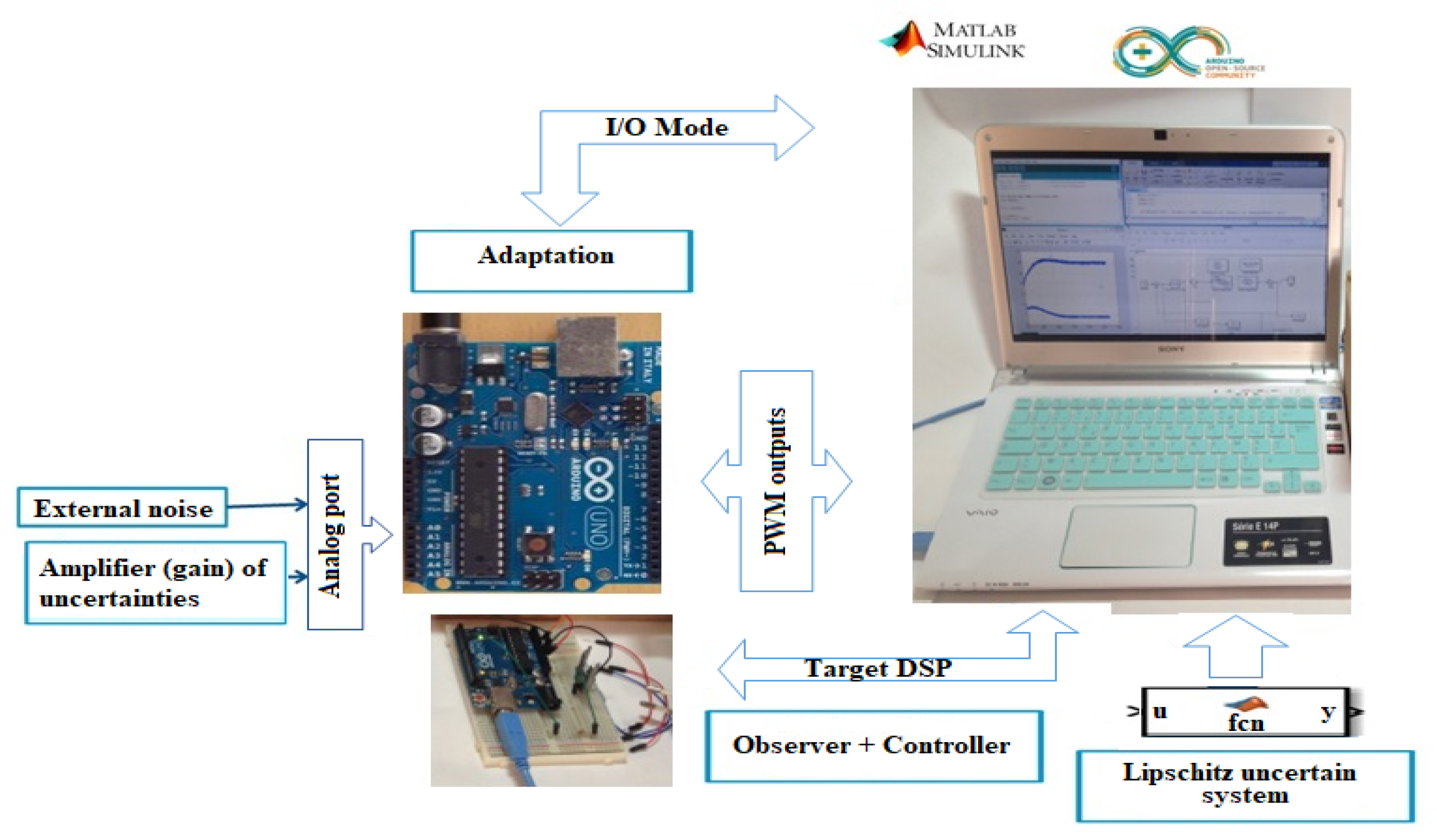
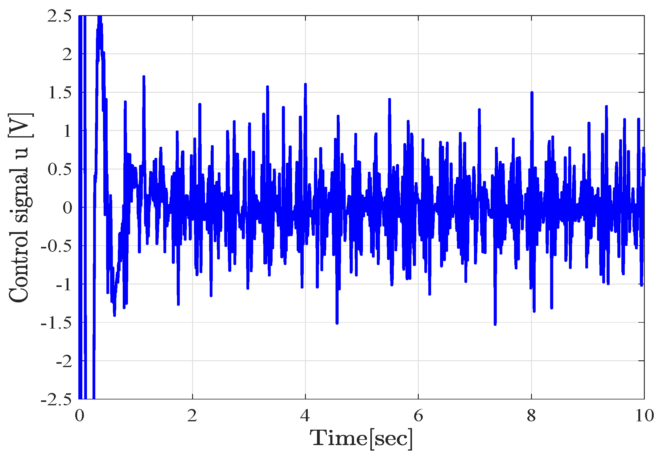
5.1.2. Experimental Results

In order to validate the proposed approach presented in this paper, a real-time implementation using ARDUINO UNO R3 board as a real-time emulator (hardware-in-the-loop), that is used as an Digital Signal Processing (DSP) emulator through target mode, is presented.
Note.All technical implementation details are explained in [8,22].
The diagram illustrating the implementation is given by Figure 1.
Figure 2 and Figure 3 present, respectively, the trajectories of the real state and its estimate and the control signal u ( k ) using the sliding window approach ( r = 2 ) . The uncertainties F ( k ) are multiplied by a randomly variable gain Γ between 0 and 5 introduced through the analog port of the Arduino board. For Figure 2a, the added noise is a sinusoidal signal variable in amplitudes ± 3.8 V and frequency-modulated (330–520 Hz). For Figure 2b, we use the same noise as in Figure 2a injected in two random intervals. For Figure 2c, the added noise is a sinusoidal signal variable in amplitudes ± 2.5 V and frequency-modulated (120–300 Hz). For Figure 2d, we inject a sinusoidal signal variable in amplitudes ± 3 V and frequency-modulated (500–700 Hz) in two random intervals.
As shown in Figure 2, the states are well estimated using the proposed design method. All the presented Figure 2a–d reveal that the proposed approach provides good robustness qualities in the presence of unknown disturbances and uncertainties, which further demonstrates the practical feasibility.

5.2. Exemple 2

Let us consider the system studied in [5]. This system is described by the state model (5) with
A = 0.2 0.1 0.4 0.6 1 0.5 0.3 0 0.3 , B = 1 3 0.4 0.5 0.6 0.4 , E 1 = 1 1 1 , C = 0 1 1 1 0 1 ,
D = 1 0 0 0 1 0 0 0 1 , E 2 = 0.2 0.2 , M 1 = 0 0 0.1 0.3 0 0.2 , N 1 T = 0 0.2 0 0 0 0.4 , M 2 = 0 0.3 0 0.8 ,
N 2 = 0 0 0 0 0 0.2 , F ( k ) = sin ( k 4 )   and   g x ( k ) = 0.1 sin x 2 ( k ) 0.2 sin x 3 ( k ) 0.3 sin x 1 ( k ) .
g x ( k ) satisfies Lemma 1 with a set of vertices
V H 33 = 0 ± 0.1 0 0 0 ± 0.2 ± 0.3 0 0 .
The class of nonlinear systems studied in this paper verify the Lipschitz property. By treating this last property in order to evaluate the obtained results with respect to some existing solid work, we consider the methods in [5,19] for comparison. The first approach [5] deals with the design of robust observer-based control using a reformulated Lipschitz property combined with a slack variable technique and some mathematical artifacts. The obtained result is in the form of LMI conditions. The second method [19] proposes LMI conditions for the observer-based H stabilization problem based on the Lyapunov theory and the use of mathematical artifacts such as matrix decomposition and Young relation.
Thus, for comparison and by solving the LMIs given by the proposed approach, the standard approach ( r = 1 ) and the approaches in [5,19], we obtain the results presented in Table 1.
It is clear that the value of λ min calculated using the sliding window approach is smaller than those calculated using the standard one, the approaches in [5,19] which confirm the superiority of the proposed design scheme. Next, the obtained gain matrices using the standard approach and sliding window approach ( r = 2 ):
  • Standard approach:
    L = 0.4034 0.1235 1.1556 0.3755 0.2140 0.0923 , K = 0.3407 0.0351 0.1467 0.2555 0.1046 0.1331 .
  • Sliding window approach ( r = 2 ):
    L 1 = 0.4181 0.1258 1.1749 0.3818 0.2278 0.0960 , L 2 = 0.0055 0.0030 0.0036 0.0025 0.0012 0.0003 ,
    K 1 = 0.3357 0.0392 0.1523 0.2507 0.1028 0.1311 , K 2 = 0.0000 0.0000 0.0005 0.0000 0.0000 0.0042 .
The simulation results using the sliding window approach are given in Figure 4 for x ( 0 ) = 10 7 5 T and x ^ ( 0 ) = 1 4 1.5 T . The considered disturbance is equal to 1 and injected for 2 s < t < 3 s .
Figure 4 shows that the proposed control law with the sliding window ensures the stability of the system with reduced amplitudes and perturbations. The result can be further improved by increasing the width of the sliding measurement window (r).

6. Conclusions

In this paper, a new robust observer-based stabilization design methodology for a class of Lipschitz discrete-time systems with parametric uncertainties in a noisy context has been presented. The proposed controller is intended not only to reduce the effect of external noise, but also to be robust regarding all the uncertainties present in the model under study. The proposed new strategy introduces two sliding windows of delayed measurements and states, respectively, into the standard structures of the Luenberger observer and the estimated state feedback control law which allows to get relaxed LMI conditions. A judicious use of Young’s lemma combined with a particular slack variable allows to enhance the obtained optimization problem. Numerical results and real-time implementation with DSP device board used as an emulator are presented to validate the proposed scheme compared to existent methods.

Author Contributions

Conceptualization and methodology, N.G. and M.B.; software, N.G., A.T. and G.B.H.F.; supervision and validation, M.B. and M.A.; writing—original draft preparation, N.G.; writing—review and editing, G.B.H.F. and A.T. All authors have read and agreed to the published version of the manuscript.

Funding

This research received no external funding.

Conflicts of Interest

The authors declare no conflict of interest.

References

  1. Ho, D.; Lu, G. Robust stabilization for a class of discrete-time nonlinear systems via output feedback: The unified LMI approach. Int. J. Control 2003, 76, 105–115. [Google Scholar] [CrossRef]
  2. Auriol, J.; Di Meglio, F. Robust output feedback stabilization for two heterodirectional linear coupled hyperbolic PDEs. Automatica 2020, 115, 108896. [Google Scholar] [CrossRef]
  3. Kheloufi, H.; Bedouhene, F.; Zemouche, A.; Alessandri, A. Observer-based stabilisation of linear systems with parameter uncertainties by using enhanced LMI conditions. Int. J. Control 2015, 88, 1189–1200. [Google Scholar] [CrossRef] [Green Version]
  4. Monnet, D.; Ninin, J.; Clement, B. A global optimization approach to H synthesis with parametric uncertainties applied to AUV control. In Proceedings of the IFAC World Congress, Toulouse, France, 9–14 July 2017; pp. 3953–3958. [Google Scholar]
  5. Kheloufi, H.; Zemouche, A.; Bedouhene, F.; Souley-Ali, H. A robust H observer-based stabilization method for systems with uncertain parameters and Lipschitz nonlinearities. Int. J. Robust Nonlinear Control 2016, 26, 1962–1979. [Google Scholar] [CrossRef]
  6. Song, J.; He, S. Robust finite-time H control for one-sided Lipschitz nonlinear systems via state feedback and output feedback. J. Frankl. Inst. 2015, 352, 3250–3266. [Google Scholar] [CrossRef]
  7. Ito, H.; Dinh, T.N. Interval observers for global feedback control of nonlinear systems with robustness with respect to disturbances. Eur. J. Control 2018, 39, 68–77. [Google Scholar] [CrossRef]
  8. Thabet, A.; Frej, G.B.H.; Boutayeb, M. Observer-based feedback stabilization for lipschitz nonlinear systems with extension to H performance analysis: Design and experimental results. IEEE Trans. Control Syst. Technol. 2018, 26, 321–328. [Google Scholar] [CrossRef]
  9. Shao, K.; Zheng, J.; Huang, K.; Wang, H.; Man, Z.; Fu, M. Finite-Time Control of a Linear Motor Positioner Using Adaptive Recursive Terminal Sliding Mode. IEEE Trans. Ind. Electron. 2020, 67, 6659–6668. [Google Scholar] [CrossRef]
  10. Shao, K.; Zheng, J.; Wang, H.; Wang, X.; Lu, R.; Man, Z. Tracking Control of a Linear Motor Positioner Based on Barrier Function Adaptive Sliding Mode. IEEE Trans. Ind. Inform. 2021, 17, 7479–7488. [Google Scholar] [CrossRef]
  11. Mao, X.; Liu, W.; Hu, L.; Luo, Q.; Lu, J. Stabilization of hybrid stochastic differential equations by feedback control based on discrete-time state observations. Syst. Control Lett. 2014, 73, 88–95. [Google Scholar] [CrossRef] [Green Version]
  12. Gasmi, N.; Boutayeb, M.; Thabet, A.; Aoun, M. Enhanced LMI Conditions for Observer-Based H Stabilization of Lipschitz Discrete-Time Systems. Eur. J. Control 2018, 44, 80–89. [Google Scholar] [CrossRef]
  13. Scholtz, E. Observer Based Monitors and Distributed Wave Controllers for Electromechanical Disturbances in Power Systems. Ph.D. Thesis, Massachusetts Institute Technology, Cambridge, MA, USA, 2004. [Google Scholar]
  14. Ibrir, S.; Xie, W.F.; Su, C.Y. Observer-based control of discrete-time Lipschitzian non-linear systems: Application to one-link flexible joint robot. Int. J. Control 2005, 78, 385–395. [Google Scholar] [CrossRef]
  15. Grandvallet, B.; Zemouche, A.; Boutayeb, M.; Changey, S. A sliding window filter for real-time attitude independent TAM calibration. In Proceedings of the 49th IEEE Conference on Decision and Control, Atlanta, GA, USA, 15–17 December 2010; pp. 467–472. [Google Scholar]
  16. Lin, W.; Byrnes, C. Remarks on linearization of discrete-time autonomous systems and nonlinear observer design. Syst. Control Lett. 1995, 25, 31–40. [Google Scholar] [CrossRef]
  17. Rajamani, R. Observer for Lipschitz nonlinear systems. IEEE Trans. Autom. Control 1998, 43, 397–401. [Google Scholar] [CrossRef]
  18. Ibrir, S. Static output feedback and guaranteed cost control of a class of discrete-time nonlinear systems with partial state measurements. Nonlinear Anal. Theory Methods Appl. 2008, 68, 1784–1792. [Google Scholar] [CrossRef]
  19. Grandvallet, B.; Zemouche, A.; Souley-Ali, H.; Boutayeb, M. New LMI Condition for Observer-Based H Stabilization of a Class of Nonlinear Discrete-Time Systems. SIAM J. Control Optim. 2013, 51, 784–800. [Google Scholar] [CrossRef]
  20. Heemels, W.; Daafouz, J.; Millerioux, G. Observer-Based Control of Discrete-Time LPV Systems With Uncertain Parameters. IEEE Trans. Autom. Control 2010, 55, 2130–2135. [Google Scholar] [CrossRef] [Green Version]
  21. Grandvallet, B.; Zemouche, A.; Boutayeb, M.; Changey, S. Real-Time Attitude-Independent Three-Axis Magnetometer Calibration for Spinning Projectiles: A Sliding Window Approach. IEEE Trans. Control Syst. Technol. 2014, 22, 255–264. [Google Scholar] [CrossRef]
  22. Gasmi, N.; Boutayeb, M.; Thabet, A.; Aoun, M. Sliding Window Based Nonlinear H Filtering: Design and Experimental Results. IEEE Trans. Circuits Syst. II Express Briefs 2019, 66, 302–306. [Google Scholar] [CrossRef]
  23. Zemouche, A.; Rajamani, R.; Phanomchoeng, G.; Boulkroune, B.; Rafaralahy, H.; Zasadzinski, M. Circle criterion-based H observer design for Lipschitz and monotonic nonlinear systems–Enhanced LMI conditions and constructive discussions. Automatica 2017, 85, 412–425. [Google Scholar] [CrossRef] [Green Version]
  24. Ibrir, S.; Diopt, S. Novel LMI Conditions for observer-based stabilization of Lipschitzian nonlinear systems and uncertain linear systems in discrete-time. Appl. Math. Comput. 2008, 206, 579–588. [Google Scholar] [CrossRef]
  25. Petersen, I. A stabilization algorithm for a class of uncertain linear systems. Syst. Control Lett. 1987, 8, 351–357. [Google Scholar] [CrossRef]
  26. Spong, M. Modeling and control of elastic joint robots. Trans. ASME J. Dyn. Syst. Meas. Control 1987, 109, 310–319. [Google Scholar] [CrossRef]
Figure 1. Block diagram of real-time implementation.
Actuators 10 00303 g001
Figure 2. Evolution of the states (solid line) and their estimates (dashed line): (a) Behavior of x 1 and its estimate, (b) Behavior of x 2 and its estimate, (c) Behavior of x 3 and its estimate, (d) Behavior of x 4 and its estimate.
Actuators 10 00303 g002
Figure 3. Evolution of the control signal u.
Actuators 10 00303 g003
Figure 4. Evolution of the states x 1 , x 2 , x 3 (solid line) and their estimates (dashed line) using the sliding window approach.
Actuators 10 00303 g004
Table 1. Different values of λ min .
Approach λ min
Observer-Based H Stabilization approach [19]2.6777
Observer-Based H Stabilization approach [5]2.3790
Standard approach ( r = 1 )1.6052
Sliding window approach ( r = 2 )1.4551
Publisher’s Note: MDPI stays neutral with regard to jurisdictional claims in published maps and institutional affiliations.

