Interval Type-2 Fuzzy Dynamic High Type Control of Permanent Magnet Synchronous Motor with Vector Decoupling Method

Abstract

This paper presents an interval type-2 fuzzy dynamic high type (IT2FDHT) control based on vector decoupling method for permanent magnet synchronous motor (PMSM) to improve the dynamic characteristics of the system. Firstly, to address the shortcomings of the traditional PI regulator used in the current loop of PMSM, an improved PI regulator based on voltage feed-forward decoupling is used. Then, considering the characteristics that the higher the system type, the smaller the steady-state error and the shorter the regulation time, the high type control structure is added. However, a purely high type structure amplifies the oscillations of the system and is extremely sensitive to perturbations, which can easily lead to system divergence. Therefore, in order to solve the problems caused by high type structure, finally we designed dynamic high type control with the help of fuzzy logic systems (FLSs), which successfully achieved automatic switching of system type while improving response speed and steady-state accuracy. Meanwhile, quantum-behaved particle swarm optimization (QPSO) algorithm is employed to determine the parameters of FLSs. In summary, five methods including conventional PI, feed-forward decoupling PI (FDPI), FDPI high type (FDPI-HT), FDPI type-1 fuzzy dynamic high type (FDPI-T1FDHT), and FDPI-IT2FDHT, are compared to show the superiority of the proposed method. By means of simulations, the excellence of proposed FDPI-IT2FDHT is verified.

1. Introduction

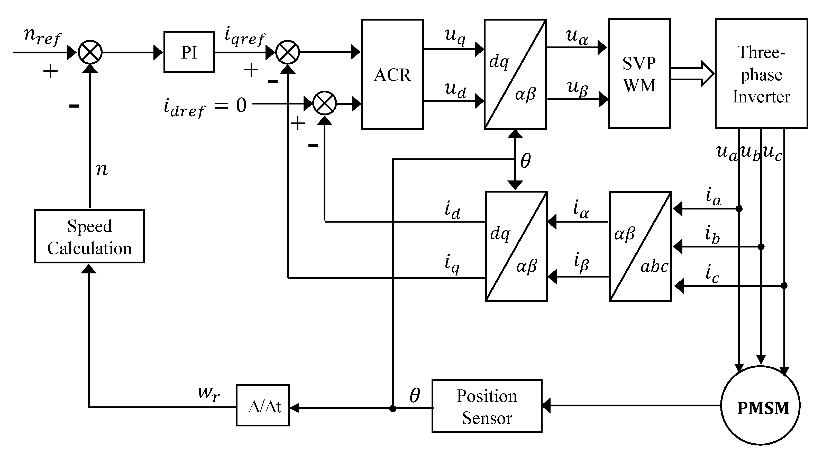
The advantages of PMSM are small size, simple structure, light weight, low losses. It does not have commutator and brushes of DC motor, and it is characterized by high efficiency, high power factor, large torque inertia ratio, small current and resistance losses, high reliability and strong coupling [1,2,3]. One of the more widely used control methods for these motors is the vector control method with rotor field orientation. The basic principle of operation is to decouple the magnetic field current and torque current of the motor on a synchronous coordinate system with rotor field orientation through coordinate transformation, so that it has the same operating performance as the conventional DC motor [4,5,6]. The vector control system of PMSM can realize high precision, high dynamic performance, and wide range of speed regulation or positioning control, so the vector control system of PMSM has attracted a lot of attention from scholars at home and abroad [7,8,9].

However, vector control only achieves the static decoupling of the two current components, not the dynamic decoupling, and the coupling voltage exists in the dynamic process, especially at high speed, the coupling voltage can even reach $30\%$ of the stator voltage [10], causing the two current components to affect each other, which makes the control performance of the system reduced. Dynamic decoupling is the compensation of coupling voltage to improve the control performance of the servo system based on the static decoupling. Here, feed-forward decoupling is used to compensate for the coupling voltage. By means of feed-forward decoupling, [11] used a predictive current control method to improve the dynamic performance of the system, but the method is strongly influenced by the motor parameters and is not robust. Ref. [12] applied a neural network decoupling control method, which required a large amount of experimental sample data for offline training and was relatively complicated to implement. Therefore, it is necessary to find a robust and easy-to-implement method, and high type control is such a method that meets the requirements.

High type control [13] mainly refers to the parallel connection of one or more integrators in the forward path of the system to increase the system type and thus improve some aspect of the system performance. The integrator is an electronic component commonly used in control circuits, whose output signal is the time product of the input signal. From the physical point of view, it can convert acceleration signal into velocity signal and velocity signal into position signal, which is an essential device in the multi-closed loop system. According to the principle of automatic control, the greater the number of integrators in the forward path of a closed-loop control system, the higher the system type [14]. Commonly used multi-closed-loop control systems are generally Type I or Type II systems. The higher the type, the smaller the steady-state error and the shorter the regulation time, but the system oscillation is also larger and extremely sensitive to disturbances, which can easily lead to system divergence [13]. In order to overcome the instability of the high type system and retain its advantages of high accuracy, researchers have tried different approaches. Tang constructed a PID-I type system by adding an integrator to the PID controller to take advantage of the large closed-loop bandwidth of the PID so that the high-type system can accommodate more disturbances [15]. Papadopoulos et al. designed an explicit analytical PID tuning rule for Type III control loop design based on the symmetric optimality criterion [16]. However, this static way of increasing the system type has the pitfall that the integral satiation may occur when there is a large or high frequency sudden change in the system input, which may prevent the actuator from working properly. To solve the problem of integral saturation in high type systems, dynamic high type techniques using FLSs are proposed, adaptively turning on or off the integrator according to the system status to achieve dynamic switching type, which can improve the tracking performance of the system while avoiding the saturation of the integrator.

FLSs have an excellent ability in dealing with various uncertainties and interferences [17,18,19]. At present, FLSs are mainly divided into type-1 FLSs (T1FLSs) and type-2 FLSs (T2FLSs). T1FLSs achieve a successful application in the area of fuzzy control because of its simple structure and convenient calculation. As the complexity and performance requirements of the control system increase, T1FLSs become increasingly inadequate to meet the control needs. Thus, T2FLSs, especially interval T2FLSs (IT2FLSs), have come into the limelight and are gradually being used in various fields [20,21,22]. In IT2FLSs, the pros and cons of the membership parameters and the related parameters of the controller are directly reflected in the control effect. Especially for the nonlinear controlled system with high complexity and high precision, traditional parameter setting methods are often difficult to meet control requirements. In addition, because the dimension and complexity of IT2FLSs are higher than those of traditional T1FLSs, it is difficult for conventional optimization methods to obtain effective parameter configuration. Intelligent optimization algorithms [23,24,25], as very popular methods in recent years, have been applied extensively for solving global optimization problems.

QPSO [25] is an intelligent optimization algorithm based on conventional PSO idea. PSO [24] was proposed on the basis of studies on the predatory behavior of birds. Although PSO has a wide range of applications, compared with QPSO, PSO has more parameters such as inertia weight w, acceleration coefficient c and scope of search space $V_{max}$ to be set, which is not conducive to finding the global optimal solution, and for some complex nonlinear systems, the lack of randomness in particle position changes makes it easy to fall into the dilemma of local optimization. Combined quantum mechanics and PSO, QPSO improves on the shortcomings of PSO. Regarding the quantum behavior of a particle, its motion state can be described according to the quantum uncertainty principle and the global optimal solution is found throughout the feasible solution space. Therefore, QPSO is a strategy with better global convergence than PSO. Here, we employed QPSO to determine optimal parameters of FLSs.

In conclusion, in this article, based on feed-forward decoupling PI, an IT2FDHT control method using QPSO is proposed to improve dynamic performance of PMSM. The main contributions of this paper are briefly summarized as follows:

(1)

Fuzzy dynamic high type methods are provided for the vector decoupling control of PMSM.

(2)

Aiming at the problem that related parameters in the IT2FLSs are difficult to determine, QPSO is employed.

(3)

In addition to the proposed method, PI, FDPI, FDPI-HT, FDPI-T1FDHT are also designed for simulations.

The remainder of the paper is structured as follows. Section 2 introduces PMSM mathematical model and vector control in summary. Considering PMSM traditional control methods, conventional PI and FDPI are provided in Section 3. Next, in Section 4, we will focus on fuzzy dynamic high type methods for PMSM control. Then, in Section 5, simulation analyses regarding PMSM are performed to demonstrate the excellence of FDPI-IT2FDHT method. Finally, Section 6 provides the conclusion as well as future work.

2. PMSM Mathematical Model and Vector Control

In this section, the PMSM mathematical model is introduced first, then the most commonly used vector control method is succinctly reviewed.

2.1. PMSM Mathematical Model

The PMSM is a multivariable coupled system. In order to realize the decoupling of the mathematical model of the PMSM, the mathematical model under d-q coordinates is normally used, which is convenient to analyze the steady-state and dynamic performance of the PMSM. So, when building a mathematical model of a PMSM, it is usually necessary to ignore some parameters that have little influence on the building of the mathematical model to simplify the analysis, and the following assumptions are generally made [26]:

(1)

Neglecting the saturation of the motor core;

(2)

Excluding eddy current and hysteresis losses in the motor;

(3)

The current in the motor is a symmetrical three-phase sine wave current.

Under the above conditions, the mathematical model of PMSM in a two-phase rotating coordinate system (d-q) can be obtained as

$$u_d=R_s{i}_d+\frac{d{\psi }_d}{dt}-w_r{\psi }_q$$

(1)

$$u_q=R_s{i}_q+\frac{d{\psi }_q}{dt}+w_r{\psi }_d$$

(2)

$${\psi }_d={\psi }_f+L_d{i}_d$$

(3)

$${\psi }_q=L_q{i}_q$$

(4)

$$T_e=\frac{3}{2}{p}_n\left[{\psi }_f{i}_q+\left(L_d-L_q\right)i_d{i}_q\right]$$

(5)

where $u_d$, $u_q$, $i_d$, $i_q$, $L_d$, $L_q$, ${\psi }_d$, and ${\psi }_q$ are the stator voltage, current, inductance, and flux linkage in the d-q coordinate system, respectively; $R_s$ is the stator resistance; ${\psi }_f$ is the permanent flux linkage; $w_r$ is the rotor electric angular velocity; $p_n$ is the pole pairs; $T_e$ is the electromagnetic torque.

Substituting the stator flux linkage Equations (3) and (4) into the stator voltage Equations (1) and (2)

$$\left\{\begin{array}{c}{u}_d=R_s{i}_d+L_d\frac{d{i}_d}{dt}-w_r{L}_q{i}_q\\ u_q=R_s{i}_q+L_q\frac{d{i}_q}{dt}+w_r\left(L_d{i}_d+{\psi }_f\right)\end{array}\right.$$

(6)

As can be seen from Equation (6), the stator inductance parameter causes cross-coupling in the d-q axis, and the larger the $w_r$ is the stronger the coupling effect, and its influence is greater in the variable speed and high speed regions.

2.2. PMSM Vector Control

From the mathematical model of the PMSM, it is clear that the control of the electromagnetic torque can ultimately be reduced to the control of the d-axis current and the q-axis current, with constant system parameters. For a given output torque, there are many different combinations of d-axis current (excitation current) and q-axis current (torque current), and the different combinations will affect the system efficiency, power factor, motor terminal voltage and torque output capability, thus forming the current control strategy problem of the PMSM. Usually, the control strategy of $i_d=0$ is adopted in the PMSM vector control system. The control method of $i_d=0$ is relatively simple, the electromagnetic torque and $i_q$ are linear, there is no direct axis armature reaction, no demagnetization effect, all current of the motor is used to generate electromagnetic torque, and the current control efficiency is high [27].

The structure of the PMSM vector control system is given in Figure 1. The system adopts a double closed-loop control structure with an internal current loop and an external speed loop. The position information detected by the position sensor is converted into the motor speed and compared with the reference speed to get the deviation number. This deviation signal is passed through the speed PI regulator to obtain the current torque component reference $i_{qref}$, and the stator current excitation component $i_{dref}$. The stator three-phase currents $i_a,i_b,i_c$ measured by the phase current detection circuit are converted to $i_d,i_q$ in the d-q coordinate system as the current loop feedback quantity through coordinate transformation.

The deviation signals obtained by comparing $i_{dref},i_{qref}$ with $i_d,i_q$ are passed through the automatic current regulator (ACR) to obtain the voltage signals $u_d,u_q$ in the d-q coordinate system. The voltage signals in the two-phase stationary coordinate system $u_{\alpha },u_{\beta }$ are obtained by the Park inverse transformation and fed into the SVPWM algorithm to generate control pulses, which are used to control the switching state of the three-phase inverter and thus obtain the actual current of the three-phase symmetric winding of the control stator. In this control system, the outer speed loop generates the reference value of the stator current torque component and the inner current loop gets the actual control signal, thus forming a complete speed-current double closed-loop control system.

3. PMSM Traditional Control Methods

In this section, two classic approaches, namely PI and FDPI, are presented for the design of ACR.

3.1. Conventional PI

The conventional current control scheme uses two PI regulators for independent control of the d-q axis current. Here, the current regulator design of $i_q$ channel is used as an example, and the current closed-loop control block diagram is shown in Figure 2.

The first link in Figure 2 is the PI regulator, the second is the delay model, the third is the PWM model, and the fourth is the control object PMSM model. Their transfer functions can be expressed as follows, respectively.

$$G_{ACR}=K_p+\frac{K_i}{s}$$

(7)

$$G_{delay}=\frac{1}{T_{s}s+1}$$

(8)

$$G_{PWM}=\frac{K_{PWM}}{0.5T_{s}s+1}$$

(9)

$$G_{plant}=\frac{i_q}{u_q}=\frac{1}{L_{q}s+R_s}$$

(10)

where $K_p$, $K_i$ are the coefficients of the PI regulator, $T_s$ is the current sampling filter time constant, $K_{PWM}$ is the amplification of PWM, $L_q$ is the stator inductance and $R_s$ is the stator resistance. Due to the high sampling frequency of the current, the delay link and the PWM link can be combined and processed, and then after letting $K_{PWM}=1$ we can get

$$G_{delay}·G_{PWM}=\frac{1}{0.5{T_s}^2{s}^2+1.5T_{s}s+1}\approx \frac{1}{1.5T_{s}s+1}$$

(11)

At this point, the current loop in Figure 2 is adjusted according to a typical type-1 system [28], the open-loop transfer function is

$$G_{open}=\frac{K_p(\tau s+1)}{\tau s}\frac{1}{R_s(\frac{L_q}{R_s}s+1)}\frac{1}{1.5T_{s}s+1}=\frac{K}{s(Ts+1)}$$

(12)

If we make $\tau =\frac{L_q}{R_s}$, we can obtain the rectified open-loop transfer function

$$G_{open}=\frac{K_p}{R_s\tau s(1.5T_s+1)}=\frac{K}{s(Ts+1)}$$

(13)

Solving for K and T according to Equation (13)

$$K=\frac{K_p}{R_s\tau }=\frac{K_p}{L_q}$$

(14)

$$T=1.5T_s$$

(15)

In order to make the current loop have fast response without large overshoot, it is designed as a typical type-1 system according to the engineering design method, and the damping factor is taken as 0.707, then $KT=0.5$, and thus the coefficients of the PI regulator can be found [28].

$$K_p=\frac{L_q}{3T_s}$$

(16)

$$K_i=\frac{K_p}{\tau }=\frac{K_p{R}_s}{L_q}=\frac{R_s}{3T_s}$$

(17)

Considering the actual speed regulation system power supply rated voltage, rated current and other constraints, it is necessary to choose an anti-integration saturation PI regulator that limits the output quantity of the regulator and the internal integrator. The conventional PI current regulator is simple in structure and easy to implement, but ignores the influence of the d-q axis cross-coupling and only does the steady-state approximation coupling. The effect of the cross-coupling term is speed-dependent, and the coupling effect is significant during the speed regulation or in the high-speed section, which cannot meet the performance requirements by relying only on the PI regulator for current regulation.

3.2. Feed-Forward Decoupling PI

From Equation (6), it can be seen that there is a coupling term in the state equation when a conventional PI regulator is used. Part of the output voltage of the conventional PI regulator is used to offset the counter-electromotive force. Part of it is used to control the cross-direct axis current, which increases the regulation time and reduces the regulation accuracy and the dynamic performance of the system [29]. Therefore, by compensating the coupling term in Equation (18) in the conventional current regulator, the dynamic performance of the system can be improved.

$$\left\{\begin{array}{c}{u_d}^{\prime }=u_d+w_r{L}_q{i}_q\\ {u_q}^{\prime }=u_q-w_r{L}_d{i}_d-w_r{\psi }_f\end{array}\right.$$

(18)

Substituting Equation (18) into Equation (6) yields

$$\left\{\begin{array}{l}{u_d}^{\prime }=R_s{i}_d+L_d\frac{d{i}_d}{dt}\\ {u_q}^{\prime }=R_s{i}_q+L_q\frac{d{i}_q}{dt}\end{array}\right.$$

(19)

According to the above equation, it can be seen that there is no coupling in the voltage equation after compensation. Figure 3 shows the structure of the voltage feed-forward decoupled compensated current regulator design.

4. Fuzzy Dynamic High Type Methods

In this section, firstly, we will present a detailed introduction of the QPSO algorithm. Then, the focus is the design of high type (HT) and fuzzy dynamic high type (T1FDHT and IT2FDHT).

4.1. QPSO Algorithm

For an N-dimensional optimization problem, we assume that there are M particles, and the position of each particle can represent a potential solution. In the tth generation of the particle population, the N-dimensional position of the ith particle can be represented as $X_i\left(t\right)=\left(X_{i,1}\left(t\right),X_{i,2}\left(t\right),...,X_{i,N}\left(t\right)\right)$. Besides, the optimal positions of the ith particle and the particle population are denoted as $P_i\left(t\right)=\left(P_{i,1}\left(t\right),P_{i,2}\left(t\right),...,P_{i,N}\left(t\right)\right)$ and $G\left(t\right)=(G_1\left(t\right),G_2\left(t\right),...,G_N\left(t\right))$, respectively. $P_i\left(t\right)$ is determined by the following equation

$$P_i\left(t\right)=\left\{\begin{array}{c}{X}_i\left(t\right),f\left(X_i\left(t\right)\right)<f\left(P_i\left(t-1\right)\right)\\ P_i\left(t-1\right),f\left(X_i\left(t\right)\right)\ge f\left(P_i\left(t-1\right)\right)\end{array}\right.$$

(20)

where the function $f\left(·\right)$ is the fitness function, and $G\left(t\right)$ is calculated by Equation (21)

$$\begin{array}{c}G\left(t\right)=P_g\left(t\right)\\ g=arg\underset{1\le i\le M}{min}\left\{f\left(P_i\left(t\right)\right)\right\}\end{array}$$

(21)

Since the position and velocity of a particle cannot be determined simultaneously in quantum space, by means of the wave function we can describe the quantum state of the particle. Finally, the improved expressions for the particle position are obtained by the Monte Carlo method

$$p_{i,j}\left(t\right)=G_j\left(t\right)+\phi ·\left(P_{i,j}\left(t\right)-G_j\left(t\right)\right)$$

(22)

$$X_{i,j}\left(t+1\right)=p_{i,j}\left(t\right)\pm \alpha ·\left|m_j\left(t\right)-X_{i,j}\left(t\right)\right|·ln\left(1/\phantom{1u}u\right)$$

(23)

where $\alpha$ is the contraction-expansion coefficient, u as well as $\phi$ are random numbers between 0 and 1, and the mean optimal position $m\left(t\right)$ is

$$m\left(t\right)=\left(m_1\left(t\right),m_2\left(t\right),...,m_N\left(t\right)\right)=\frac{1}{M}\sum _{i=1}^M{P}_i\left(t\right)$$

(24)

4.2. High Type

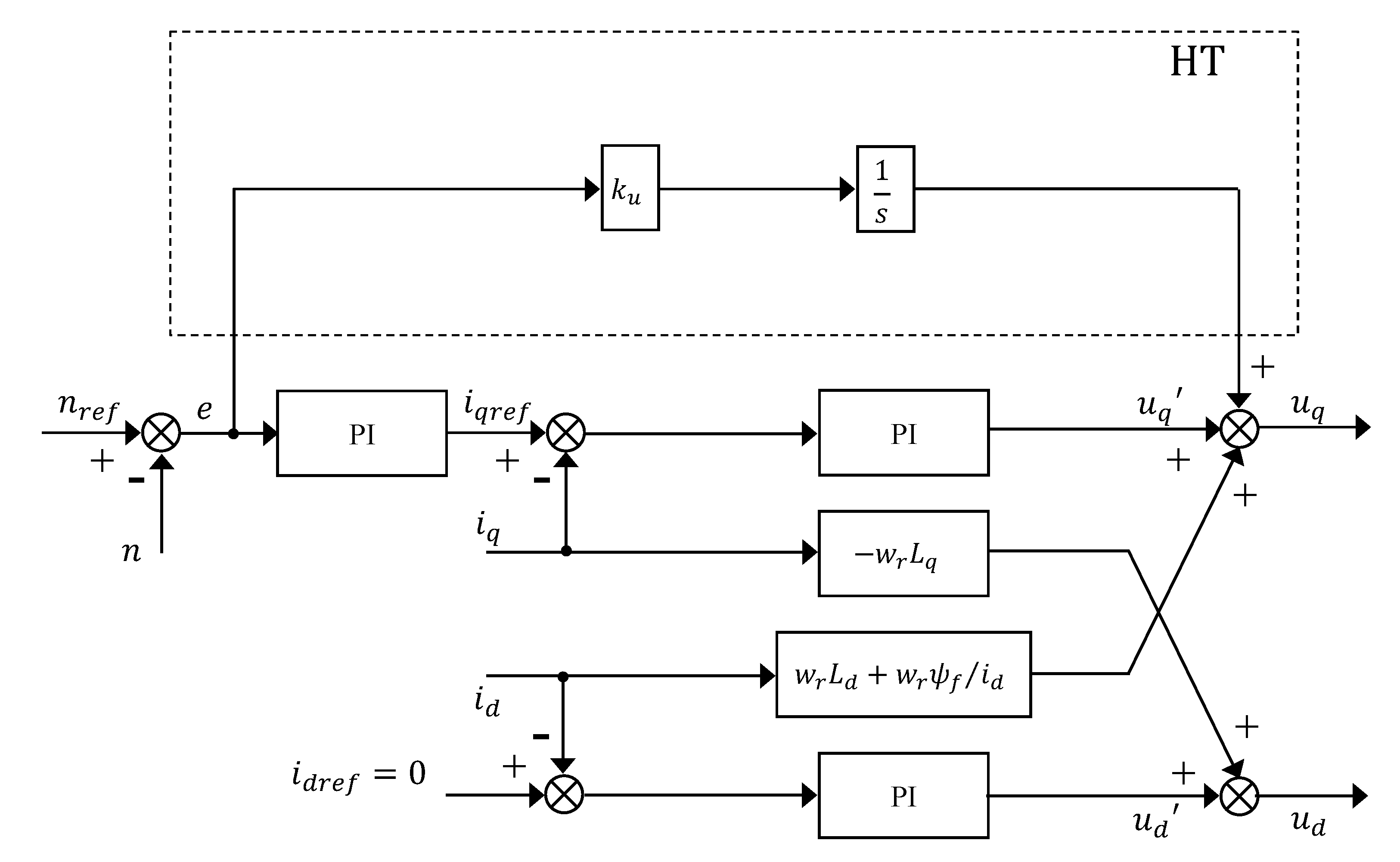
As mentioned in introduction, high type control is mainly a structure that improves the performance of a system in some way by adding one or more integrators to the forward path of the system. Figure 4 illustrates the structure of high type based on feed-forward decoupling PI, where e is speed error and $k_u$ is the amplification factor of speed error.

In order to explore the impact of high type structure on the stability and rapidity of the system, the following simulation verification schemes are designed:

1. The structure of Figure 4 is embedded in the simulation experiment of PMSM.

2. Simulation experiments are conducted with k of 10, 20, 30, 40 as well as 50 and the experimental results are compared.

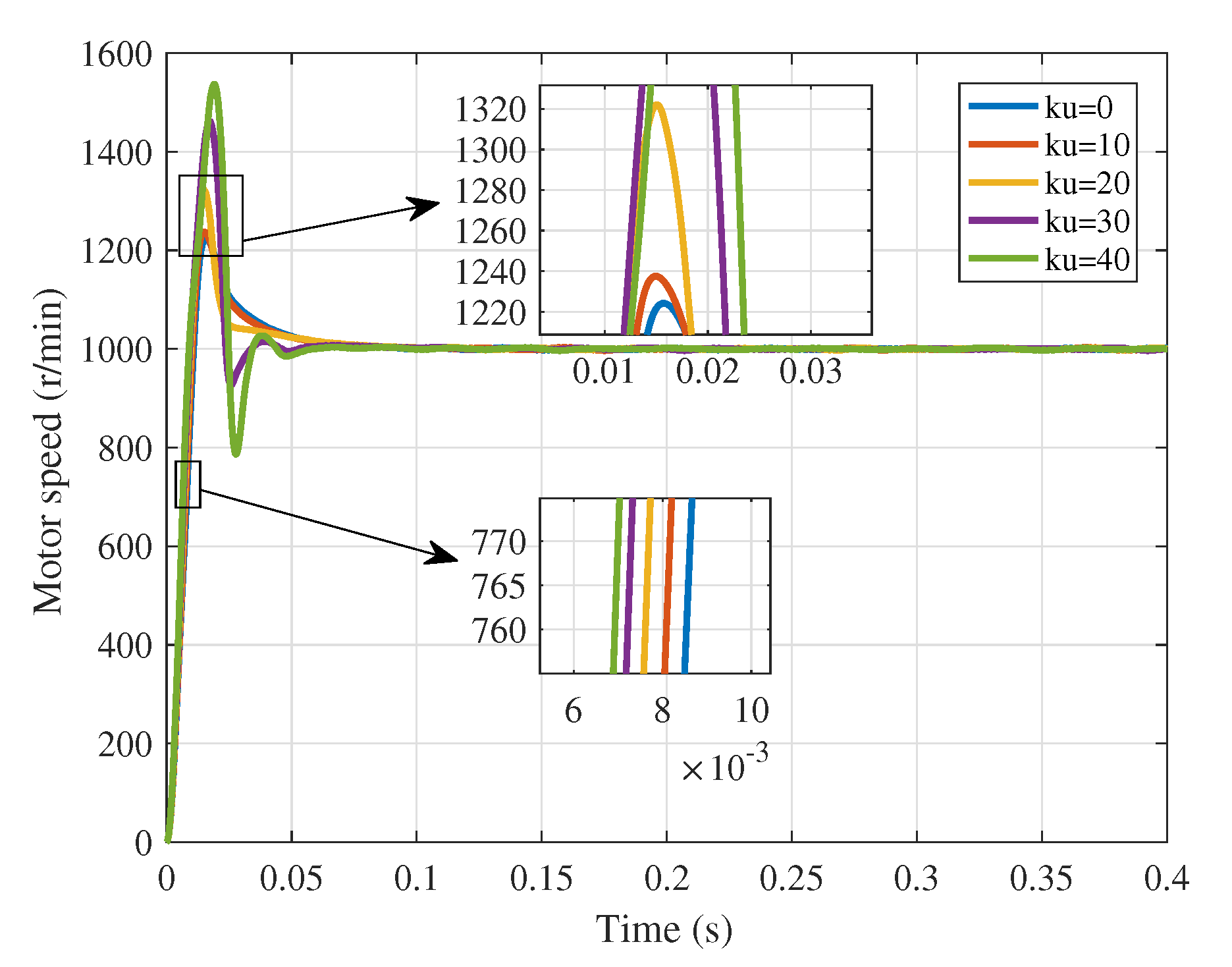
The above steps are followed to simulate and collect the data, respectively, and Figure 5 and

Table 1. Comparison of HT control indicators.

${\mathit{k}}_{\mathit{u}}$	${\mathit{t}}_{\mathit{r}}\left({10}^{-3}\mathbf{s}\right)$	${\mathit{t}}_{\mathit{s}}\left({10}^{-3}\mathbf{s}\right)$	$\mathit{\sigma }\%$
0	7.4876	38.20	22.4%
10	7.0199	35.82	23.7%
20	6.5607	24.84	32.2%
30	6.1593	27.90	46.1%
40	5.8526	32.27	53.7%

are obtained. In Table 1, $t_r$ is the rise time and represents the time required for the response curve to go from 10% to 90% of the steady-state value; $t_s$ is the regulation time, which indicates the time required for the response curve to start from zero and enter the 95–105% error band of the steady-state value; $\sigma \%$ is the overshoot, which indicates the maximum value of the response curve deviation from the steady-state value, often expressed as a percentage. Through the intuitive comparison of pictures and data, the following conclusions can be drawn.

1. The higher the system type will reduce the rise time ($t_r$), and the larger the integration gain ($k_u$), the smaller the rise time, and the faster the system will respond.

2. The higher the system type will increase the overshoot ($\sigma \%$), the larger the integral gain the larger the system overshoot will be, the more violent the oscillation will be, even leading to system divergence.

3. When the overshoot is small, the larger the integral gain, the smaller the regulation time ($t_s$). When the overshoot is large, the larger the integral gain, the larger the oscillation, and the regulation time increases.

In summary, high type control can significantly improve the rapidity of the system, but can introduce oscillations into the system, which in turn lead to high overshoot and poor regulation time, so simply increasing the system type is not a perfect solution for improving control performance.

4.3. Type-1 Fuzzy Dynamic High Type

Since the high type structure alone can lead to oscillation and even divergence problems, the dynamic high type technique was proposed. However, most of the related researches simply control the integrator on or off, and do not realize the standard of automatic switching type. In addition, the jitter caused by the switching instant is also difficult to eliminate. In the context of modernization, high demands are placed on the degree of automation and performance of PMSM, and the development of intelligent control technologies brings new possibilities for this purpose. Fuzzy logic, as one of the widely used intelligent control technologies, in combination with high type control structures, allows for automated dynamic high type control.

As can be seen from Figure 6, a T1FLS usually consists of four parts: fuzzifier, inference engine, rule base, and defuzzifier. First, the measurement inputs are processed by the fuzzifier to obtain type-1 fuzzy sets (T1FSs), and these T1FSs are mapped to all membership functions (MFs) to calculate the corresponding membership degrees. Next, the inference engine further determines the firing strengths of the rules based on the predefined rules in its rule base. After determining the membership degrees and firing strengths, the T1FSs can be calculated. Finally, a defuzzifier is used to process the output T1FSs to acquire the output of the system.

The FLS is implemented by monitoring the error and error change. So, the inputs of the FLS, i.e., E and $EC$, can be of the form

$$\begin{array}{c}E\left(k\right)=k_e·e\left(k\right)\\ EC\left(k\right)=k_{ec}·\left[e\left(k\right)-e\left(k-1\right)\right]\end{array}$$

(25)

where k is the sampling moment, $k_e$ and $k_{ec}$ are the scale coefficients of the two inputs.

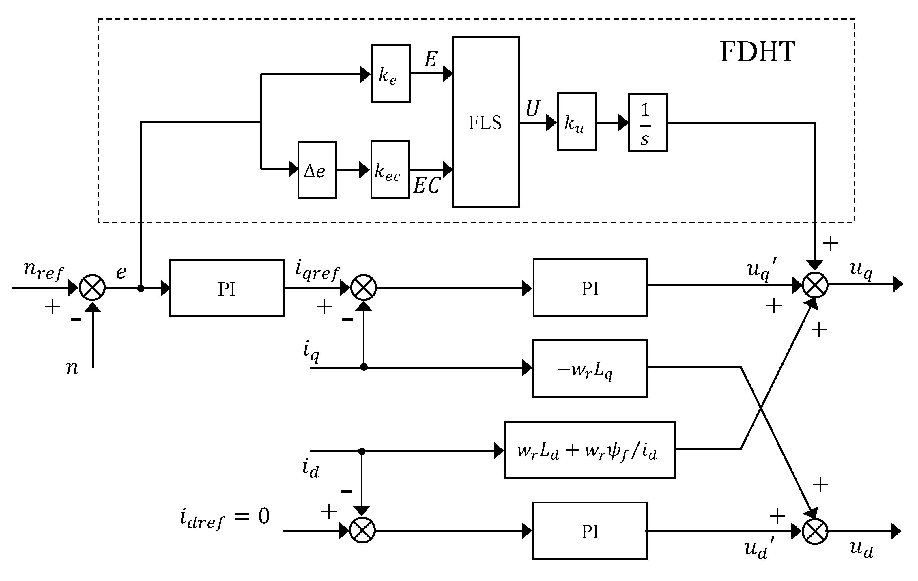
So, the structure of the fuzzy dynamic high type (FDHT) based on feed-forward decoupling PI is designed in Figure 7.

Where $\Delta e$ is the error change, U is the output of the FLS, and $k_u$ is the amplification factor of the output. By using the FLS, the oscillation problem caused by the high type structure can be handled and the dynamic switching of system types can be realized.

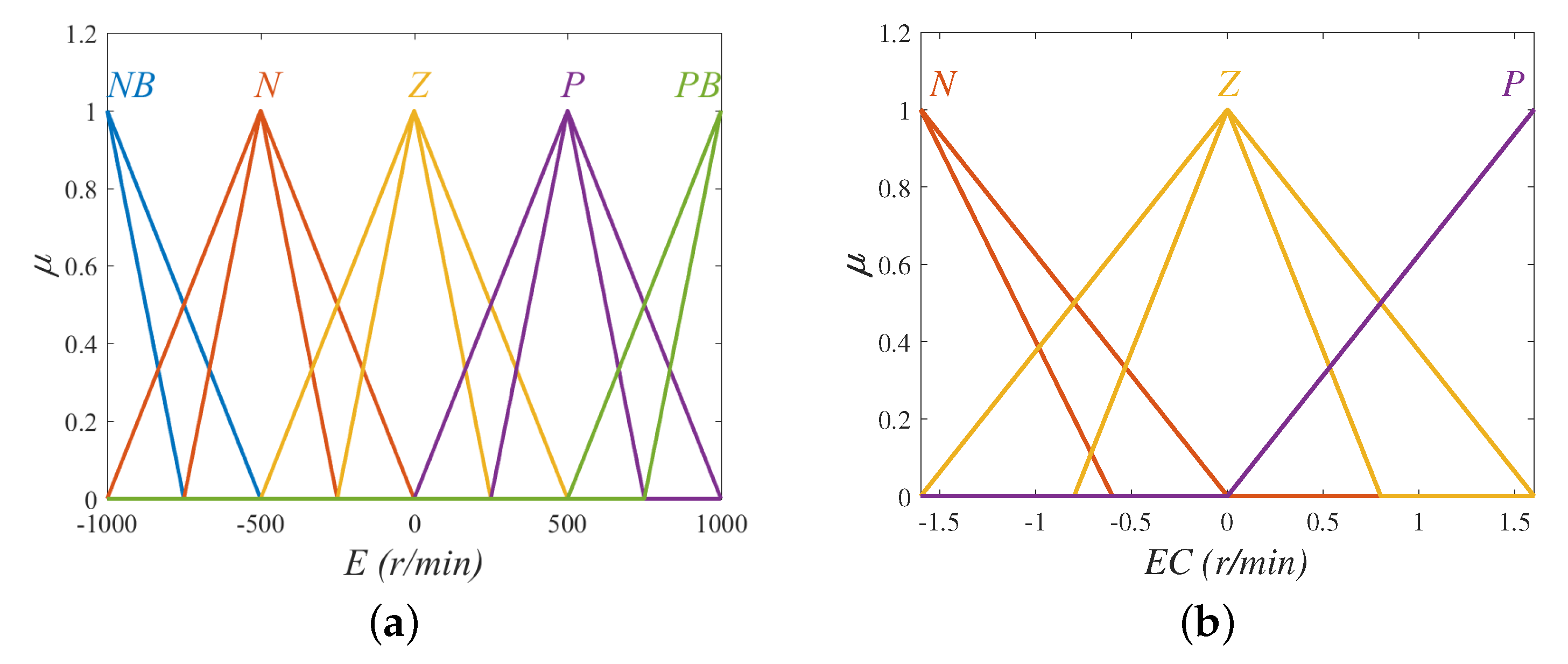
Here, we mainly describe the design of T1FLS. Figure 8a,b, respectively, display MFs of input variable E and $EC$, and Figure 8c shows MFs of output variable U.

According to Figure 8, the T-S T1FLS with two inputs and a single output has a total of 15 rules, and the i-th rule has the following form

$$R^i:IFEis{M}^{i}andECis{N}^{i}THENUis{Y}^i$$

where $Y^i$ is the consequent, $M^i$ and $N^i$ are the antecedents of the ith rule.

Through some simulations and analysis, it is found that when the output of the FLS and the error have the same sign, it will strengthen the current trend of error variation, and vice versa will weaken this trend. Thus, if $EC$ is N, when E is negative ($NB$ or N), the amount of error will be increasing and we need to suppress this tendency, so the output of the FLS takes positive (P or $PB$), with the error difference sign. If $EC$ is N, the amount of error gets smaller when E is positive ($PB$ or P), and this trend needs to be accelerated, but we find that the traditional FDPI method produces overshoot, and to avoid overshoot, the output is taken as P or Z. Similarly, to reduce overshoot or oscillation, the output of the FLS is Z or N when E is Z. For the sense of brevity, only the case where $EC$ is N is described.

Table 2. T-S fuzzy rules of the system.

Rules		E
		NB	N	Z	P	PB
EC	N	PB	PB	N	Z	P
	Z	P	Z	Z	PB	PB
	P	N	N	Z	N	N

lists the specific fuzzy rules of the T-S T1FLS.

By means of T1FLS, the T1FDHT based on FDPI, i.e., FDPI-T1FDHT, not only has a faster dynamic response, but can also handle a wide range of loads and perturbations. Nevertheless, faced with higher performance requirements and more load devices of PMSM, FDPI-T1FDHT is hardly perfect for the job.

4.4. Interval Type-2 Fuzzy Dynamic High Type

Figure 9 is the structure diagram of an IT2FLS. Compared with T1FLS in Figure 6, the main difference is that IT2FLS has an additional step of type-reduction. The role of type-reduction is to transform the T2FSs into T1FSs. Here, we use the common type-reduction inference approach, namely center-of-set (COS) type-reduction [30], to acquire T1FSs.

The input to the IT2FLS has the same form as the input to the T1FLS in Equation (25), and the only difference is the MFs of the input and output. Figure 10a,b present MFs of input variable E and $EC$ in the IT2FLS, respectively.

Table 3. The consequent MFs of output variable U in the IT2FLS.

Consequent	Range (r/min)	Consequent	Range (r/min)
N	[−35,000, −30,000]	P	[15,000, 20,000]
Z	[−10, 10]	PB	[25,000, 30,000]

shows consequent MFs of output variable U in the IT2FLS.

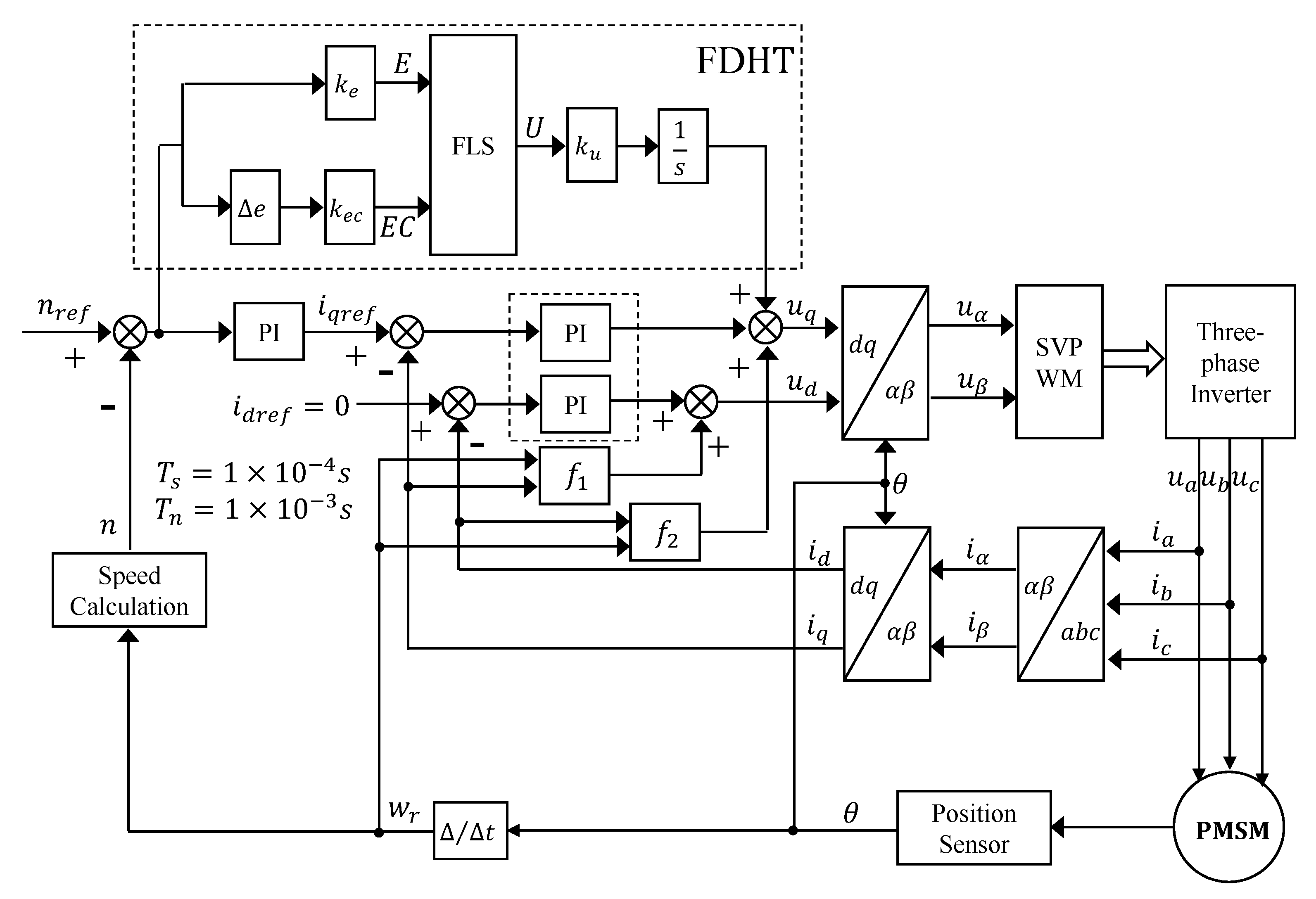
Regarding the rules, IT2FLS and T1FLS have the same design, as shown in Table 2. Eventually, we provide the structure of the PMSM vector control system applying FDPI-FDHT (FDPI-T1FDHT and FDPI-IT2FDHT) methods. The dashed box at the top of Figure 11 describes the design of FDHT, while the dashed box at the bottom of the Figure 11 shows the structure of the classic PI current regulator. $f_1$ and $f_2$ are the voltage feed-forward coupling compensation terms analyzed earlier. $T_s$ and $T_n$ are, respectively, the current sampling filter time constant and the speed sampling filter time constant [31].

Although the IT2FLS has better performance than T1FLS, the superiority of IT2FLS cannot be guaranteed if the appropriate parameters are not taken. Therefore, the relevant parameters ($k_e,k_{ec},k_u$) of the IT2FLS are optimized by the QPSO algorithm introduced earlier, while the same optimization process is adopted for the T1FLS for the sake of the reasonableness of the comparison. In the next section, we will demonstrate the excellence of FDPI-FDHT, especially FDPI-IT2FDHT, through simulation analyses.

5. Simulation Analyses

In this section, comparative simulation experiments are implemented to verify the performance of the proposed FDPI-IT2FDHT method under no-load and load conditions of the PMSM. First, the QPSO algorithm is used to optimize the relevant parameters with the motor at no load to obtain the performance comparison in that case. Then, the motor is given a proper load and then the performance change under load is tested. Finally, the analyses of the two cases is used to show the superiority of the method in this paper.

5.1. Experimental Preparation

Table 4. Parameters of the PMSM.

Parameter	Value
Pole pairs $p_n$	4
Inertia $\mathrm{J}/(\mathrm{kg}·{\mathrm{m}}^2)$	0.003
Stator resistance $R_s/\Omega$	0.958
d-axis inductance $L_d/\mathrm{mH}$	5.25
q-axis inductance $L_q/\mathrm{mH}$	12
Flux linkage ${\psi }_f/Wb$	0.1827
Viscous damping $F/(\mathrm{N}·\mathrm{m}·\mathrm{s})$	0.008
Torque constant $k_T/(\mathrm{N}·\mathrm{m}·{\mathrm{A}}^{-1})$	1.0962

lists the main parameters of the PMSM, and

Table 5. Parameters of the three PI controllers.

Parameter	Value
Speed outer loop $K_p$	0.14
Speed outer loop $K_i$	7
d-axis current inner loop $K_p$	17.5
d-axis current inner loop $K_i$	3193.3
q-axis current inner loop $K_p$	40
q-axis current inner loop $K_i$	3193.3

shows the values of parameters of the three PI controllers. To ensure that the input of the FLS, i.e., the error change, is reasonable, a discrete system is used for the analysis, where the sampling period of the system is ${10}^{-4}$ s and the total simulation time is 0.4 s.

Next, the QPSO algorithm is used to optimize the relevant parameters in FDPI-HT, FDPI-T1FDHT, and FDPI-IT2FDHT methods. After comparing Figure 4 and Figure 7, we find the high type control structure requires optimization of only one parameter ($k_u$), while the FDHT requires optimization of three parameters ($k_e,k_{ec},k_u$). So,

Table 6. Parameters used in QPSO algorithm.

Parameter	Value
Maximum generation G	100
Population size M	50
Dimension N	1 or 3
Contraction-expansion coefficient $\alpha$	[2, ..., 1]

lists the specific parameters used in QPSO algorithm.

In this table, N is the dimension, indicating the number of optimization parameters, and $\alpha$ is a contraction-expansion coefficient, which decreases linearly from 2 to 1. The choice of the fitness function in the optimization algorithm directly affects the effect of the algorithm, so the commonly used integral of absolute error (IAE) is used as the fitness function of the QPSO algorithm.

$$\mathrm{IAE}={\int }_0^{\infty }\left|e\left(t\right)\right|dt$$

(26)

To better show the prominence of the FDPI-IT2FDHT method, evaluation indicators are used to quantify the control performance of various methods. In addition to the IAE as the fitness function, the evaluation indicators also include integral of square error (ISE) and integral of time square error (ISE).

$$\mathrm{ISE}={\int }_0^{\infty }{\left|e\left(t\right)\right|}^{2}dt$$

(27)

$$\mathrm{ITSE}={\int }_0^{\infty }t{\left|e\left(t\right)\right|}^{2}dt$$

(28)

The smaller the evaluation indicators, the better the method performance. Thus, according to the above analyses, we can acquire optimization results of FDPI-HT, FDPI-T1FDHT, and FDPI-IT2FDHT methods under no-load situation in

Table 7. Optimization results of three methods under no-load situation.

Method	Optimized Parameters
FDPI-HT	$k_u=24.3158$
FDPI-T1FDHT	$k_e=1.0639,k_{ec}=1.1092,k_u=2.1819$
FDPI-IT2FDHT	$k_e=0.5888,k_{ec}=0.7088,k_u=4.1344$

.

5.2. No-Load Situation

Under no-load condition, the motor speed is set to 1000 r/min and the performance of the five methods is compared. Figure 12 and

Table 8. Evaluation indicator results under no-load situation.

Method	IAE	ITSE	ISE
PI	11.5138	28.8293	5.4714 × 103
FDPI	10.5075	23.4418	5.0137 × 103
FDPI-HT	9.8549	26.5121	5.0747 × 103
FDPI-T1FDHT	9.5774	18.0999	4.3204 × 103
FDPI-IT2FDHT	9.0851	16.0875	4.0772 × 103

, respectively, illustrate the motor speed tracking results and corresponding evaluation indicator results under no-load situation.

In Figure 12, it can be seen that compared with other methods, FDPI-IT2FDHT has the smallest overshoot and the fastest adjustment time, followed by FDPI-T1FDHT, and the worst is PI, which proves the importance of the FLS. It has been analyzed that the simple high type structure will increase the system vibration and increase the overshoot, but at the same time it will also reduce the adjustment time. Therefore, the high type structure sacrifices the overshoot in exchange for rapidity, just like the FDPI-HT simulation here. Furthermore, in Table 8, among the five methods, FDPI-IT2FDHT has the smallest evaluation index results in the no-load case, which indicates that the method performs well in all aspects. It is worth noting that the ITSE and ISE values for FDPI-HT (bolded in Table 8) are larger than those for FDPI. By analysis, this result may be caused by the excessive overshoot of FDPI-HT. However, it is its shortcomings in this respect that allow us to introduce the FLS to improve the method.

To better compare several methods, Figure 13 shows the electromagnetic torque response results in the no-load case. With the help of this figure, the superiority of the FDPI-FDHT methods, especially FDPI-IT2FDHT, can be more clearly demonstrated.

5.3. Load Situation

In the case of load, first the motor is run in no-load mode and a load torque of $10 \mathrm{N}·\mathrm{m}$ is added at time 0.2 s. The motor speed tracking and evaluation index results of five methods under load case are, respectively, shown in Figure 14 and

Table 9. Evaluation indicator results under load situation.

Method	IAE	ITSE	ISE
PI	12.7659	41.2678	5.5309 × 103
FDPI	11.7122	33.4576	5.0612 × 103
FDPI-HT	10.9804	35.3746	5.1168 × 103
FDPI-T1FDHT	10.7188	25.2505	4.3542 × 103
FDPI-IT2FDHT	10.3825	24.4755	4.1169 × 103

.

Based on Figure 14, it can be seen that all methods oscillate once the load torque is applied, while the FDPI-FDHT (FDPI-T1FDHT and FDPI-IT2FDHT) oscillate less than their counterparts. However, we find that the oscillation amplitude of FDPI-T1FDHT is smaller than that of FDPI-IT2FDHT in the face of sudden load addition. Through analysis, the reason for this phenomenon may be that the optimization parameters of FLSs are too few. This result may be avoided if some parameters of the MFs in the FLSs are not fixed. Furthermore, in Table 9, it is clear that the FDPI-FDHT methods have better performance metric results under load, which indicates their advantage in terms of resistance to load disturbances. Again, there are some outliers here (bold font in Table 9), and the cause of these outliers is most likely the overshoot of the FDPI-HT being too high.

To add variety to the comparison, the electromagnetic torque response curves under load conditions are given in Figure 15. There is no doubt that the FDPI-IT2FDHT is the fastest to track on the given torque when the load torque is added at 0.2 s, followed by the FDPI-T1FDHT, which indicates that by adding the high type structure and FLSs, the system has shorter adjustment time, faster to reach the given speed, smoother overload when adding load suddenly, and better tracking ability to the load.

Next, Figure 16 uses five subplots to show the voltage responses of $u_d$ and $u_q$ under different methods. Combined with the previous analysis, we can find that the voltage variation is closely related to the final speed tracking. The greater the change in voltage amplitude, the faster the speed change and the faster the speed response of the motor. As in Figure 16, FDPI-IT2FDHT improves the motor speed tracking by changing the voltage better compared to other methods.

Finally, the stator three-phase current variation curves under the five methods are compared. Since three current curves are to be shown for each method, the five subplots in Figure 17 are used below for comparison. Comparing these five sub-graphs, it can be seen that as the method is improved, the peak of the three-phase current also becomes larger and the time to enter the steady state becomes shorter. Specifically, the time to steady state for the five methods can be estimated from each enlarged graph, where PI is 0.035 s, FDPI is 0.026 s, FDPI-HT is 0.024 s, FDPI-T1FDHT is 0.022 s, and FDPI-IT2FDHT is 0.021 s.

In order to demonstrate more clearly the three-phase current variation of these five methods, a comprehensive comparison of each of the three currents is performed. Figure 18 displays the current variation of Ia, Ib, and Ic with each of the above five strategies. According to this figure, regardless of the current, the PI stator current takes the longest time to reach a sinusoidal wave at no-load start-up, adding voltage decoupling compensation shortens this time for the FDPI, and adopting a high type structure makes the time much shorter and the response speed faster. However, this rapidity is traded off by increasing the jitter before entering the steady state. In turn, FLSs are introduced to improve performance across the board. It is clear from the enlarged diagram the methods with fuzzy dynamic high type structure (FDPI-T1FDHT and FDPI-IT2FDHT) can enter the steady state faster whether under no load or with load.

6. Conclusions and Future Work

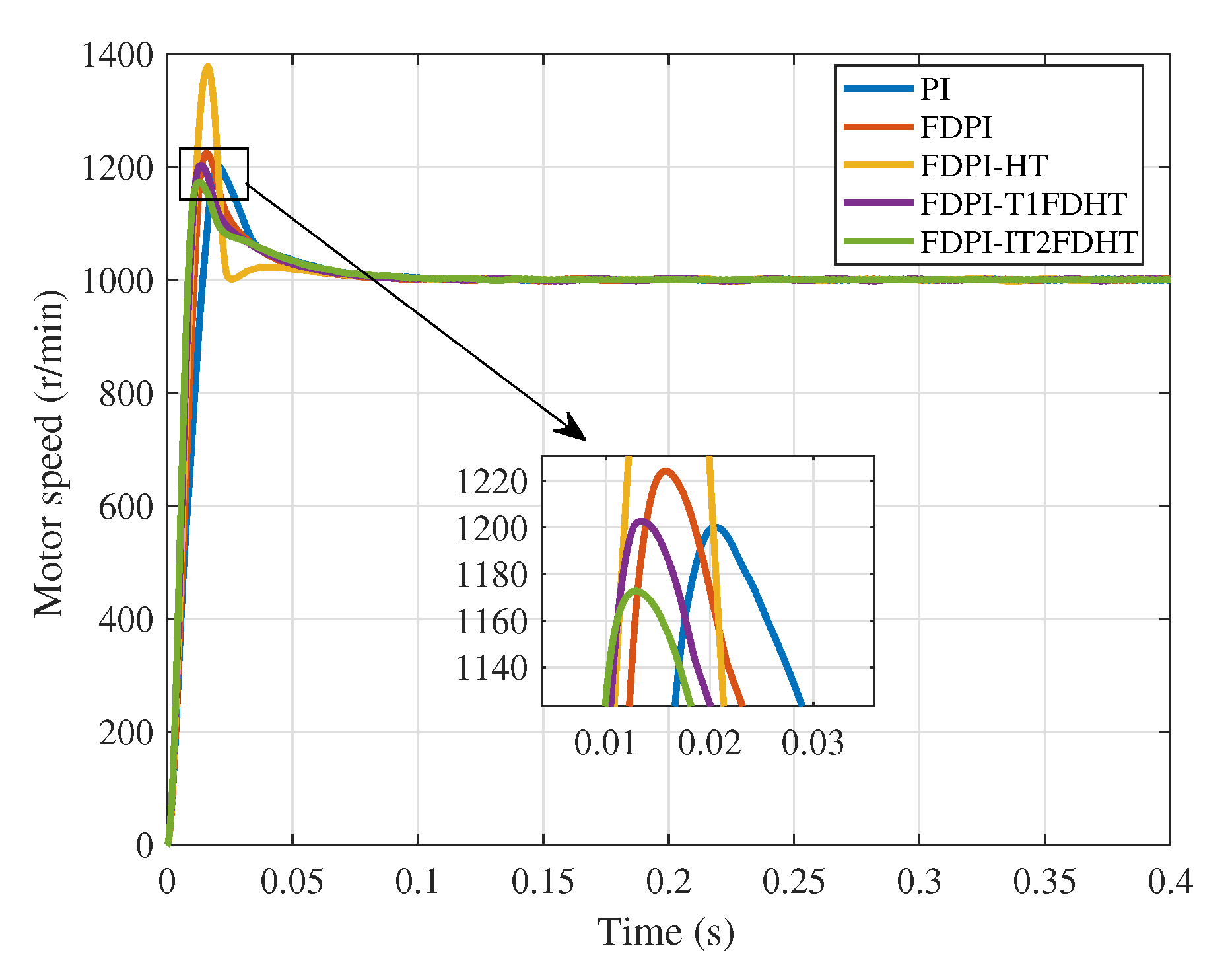
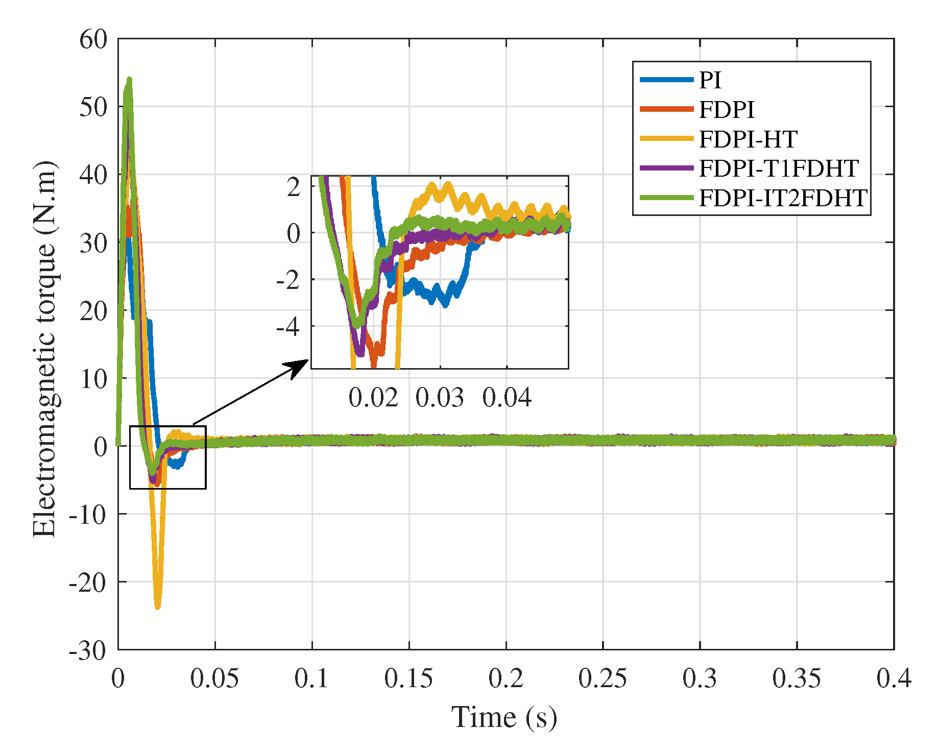
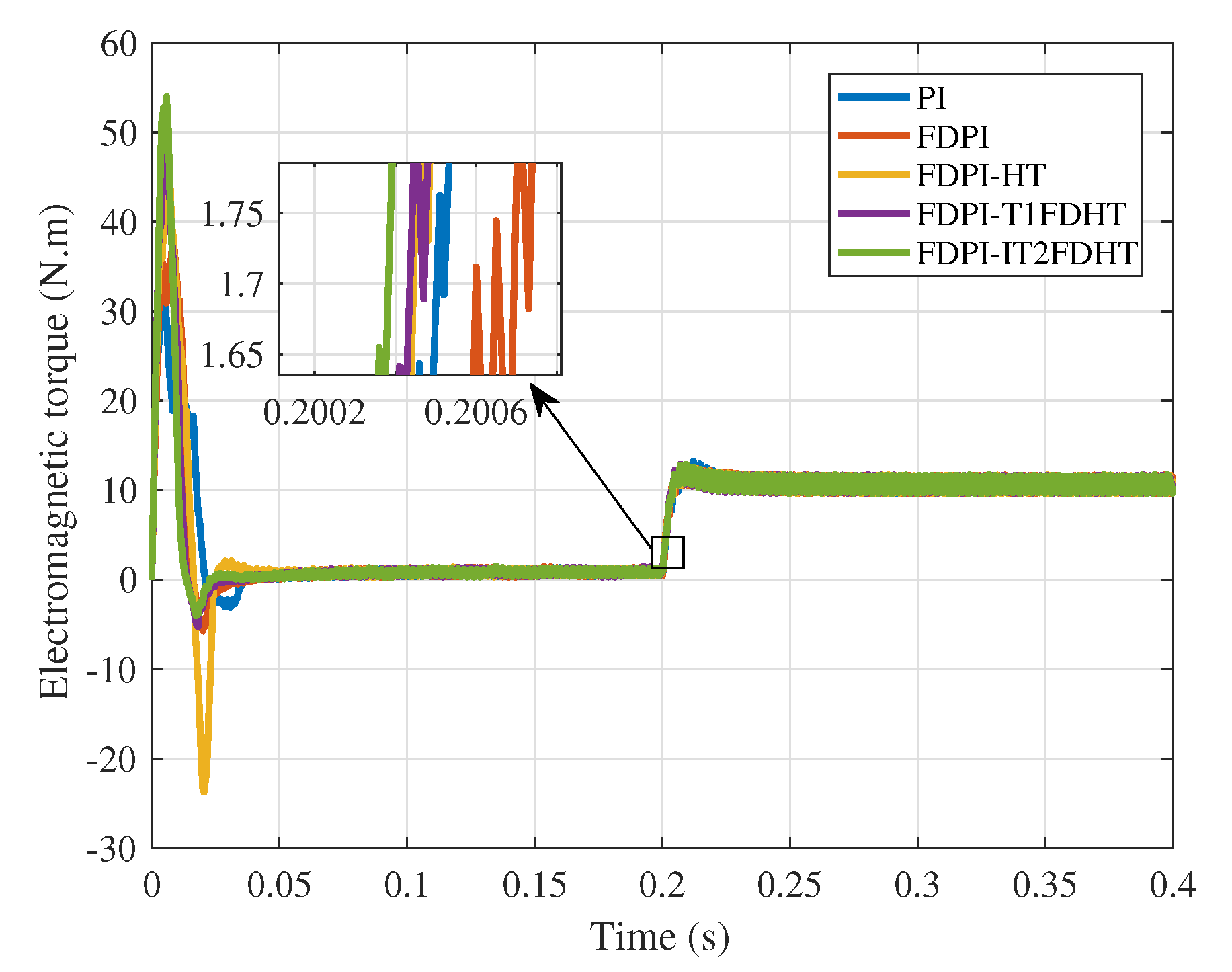
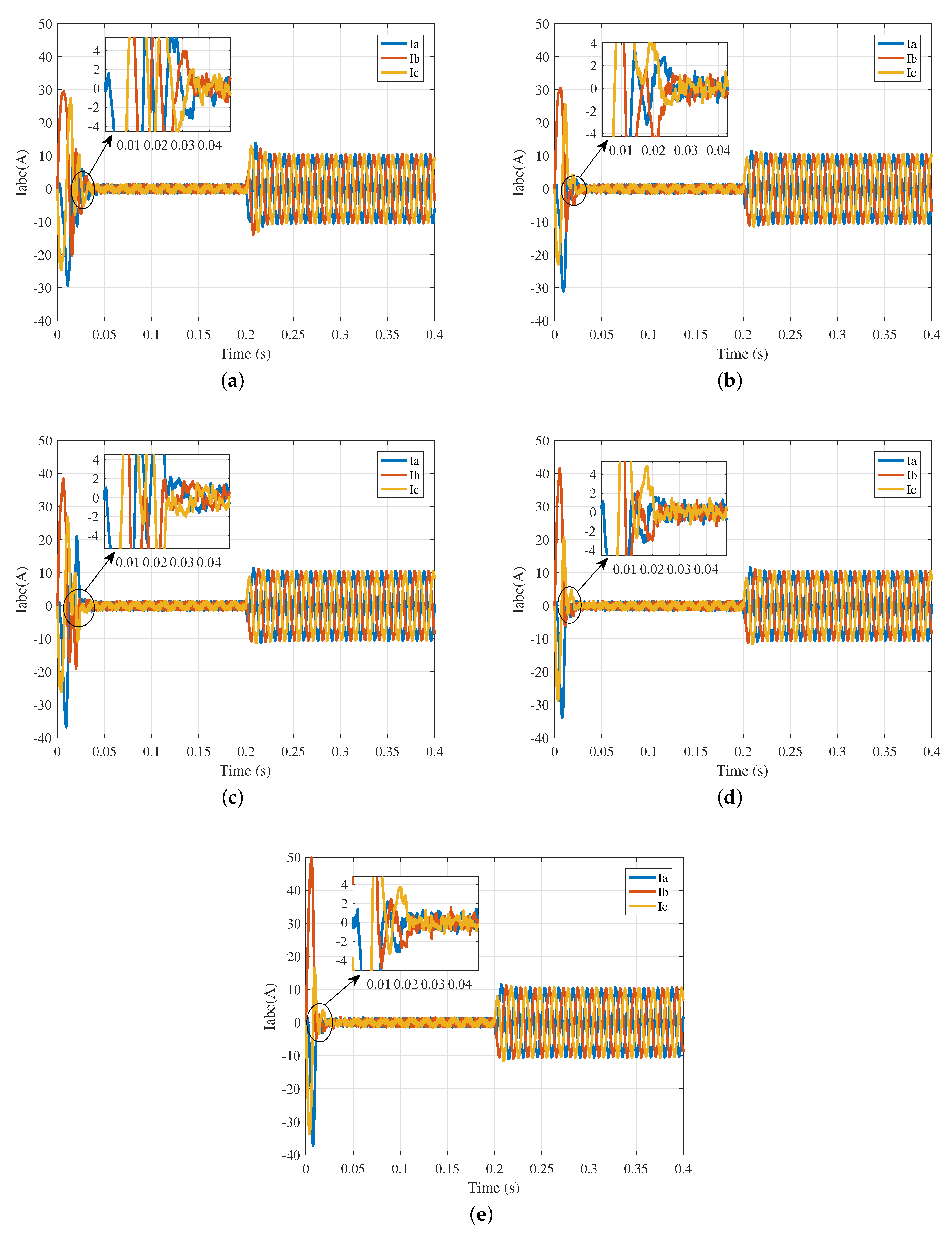
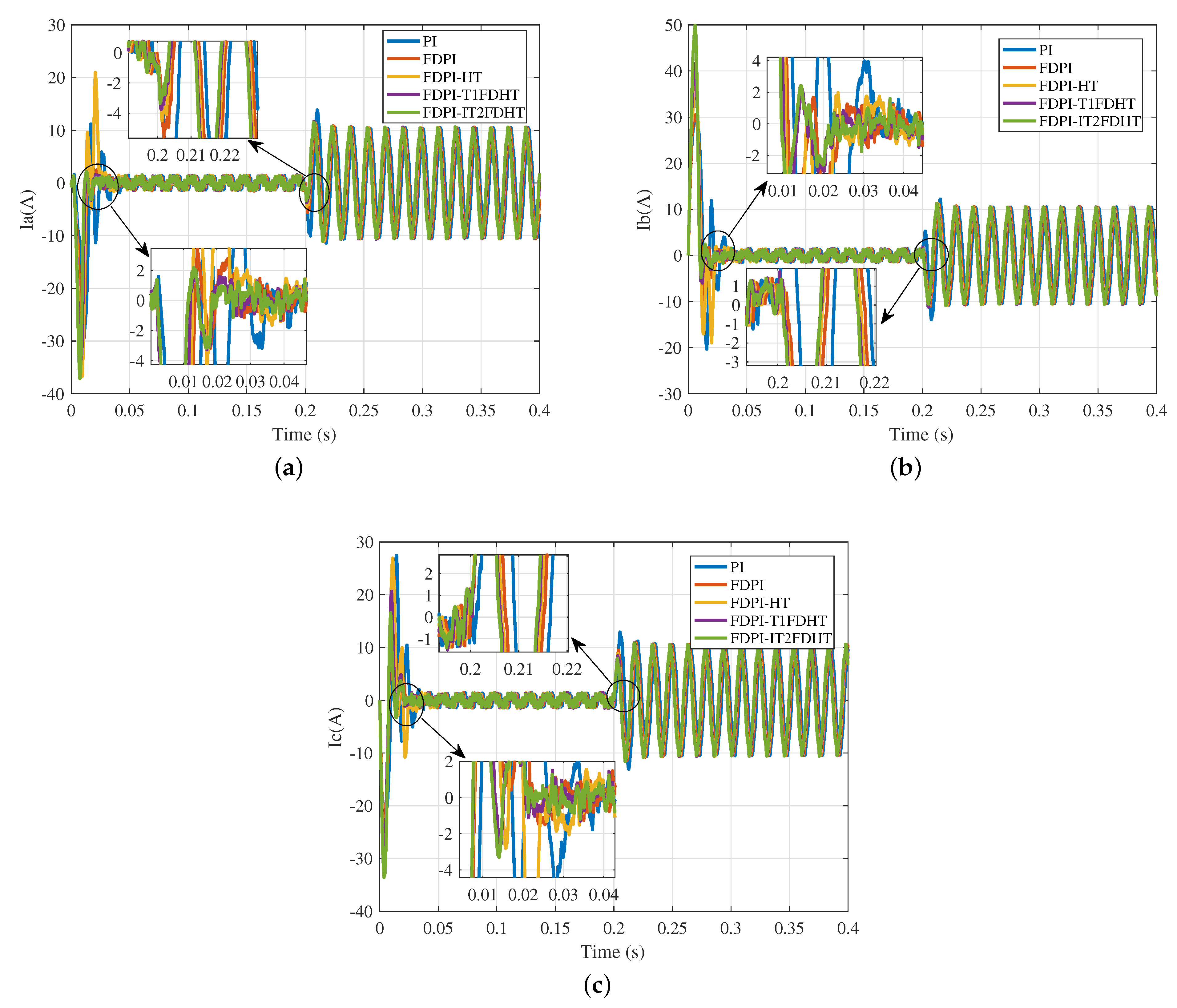
In this paper, a FDPI-IT2FDHT is proposed for PMSM to enhance the ability of dynamic response. Furthermore, to show the superiority of the designed method, PI, FDPI, FDPI-HT, and FDPI-T1FDHT are provided as well. Numerous comparative simulations suggest that FDPI with dynamic high type structure, especially FDPI-IT2FDHT, is superior to other methods in terms of dynamic characteristics and disturbance rejection, both under no-load and load conditions of the motor.

Future work will focus on improvement of FLS. Although the dynamic performance of FDPI-IT2FDHT is better than that of FDPI-T1FDHT at no load, the load oscillation of FDPI-IT2FDHT is more intense than that of FDPI-T1FDHT when a load is added, which indicates that the IT2FDHT designed in this paper is not superior to T1FDHT in all aspects and needs to be improved. Besides, we will regard experimental verification as the core of our future work.

References

1. Shi, Z.; Zhang, P.; Lin, J.; Ding, H. Permanent Magnet Synchronous Motor Speed Control Based on Improved Active Disturbance Rejection Control. Actuators 2021, 10, 147. [Google Scholar] [CrossRef]
2. Sun, X.; Shi, Z.; Lei, G.; Guo, Y.; Zhu, J. Analysis and design optimization of a permanent magnet synchronous motor for a campus patrol electric vehicle. IEEE Trans. Veh. Technol. 2019, 68, 10535–10544. [Google Scholar] [CrossRef]
3. Wang, X.; Chen, F.; Zhu, R.; Huang, X.; Sang, N.; Yang, G.; Zhang, C. A Review on Disturbance Analysis and Suppression for Permanent Magnet Linear Synchronous Motor. Actuators 2021, 10, 77. [Google Scholar] [CrossRef]
4. Rodríguez, J.; Kennel, R.M.; Espinoza, J.R.; Trincado, M.; Silva, C.A.; Rojas, C.A. High-performance control strategies for electrical drives: An experimental assessment. IEEE Trans. Ind. Electron. 2011, 59, 812–820. [Google Scholar] [CrossRef]
5. Adase, L.A.; Alsofyani, I.M.; Lee, K.B. Predictive torque control with simple duty-ratio regulator of PMSM for minimizing torque and flux ripples. IEEE Access 2019, 8, 2373–2381. [Google Scholar] [CrossRef]
6. Casadei, D.; Profumo, F.; Serra, G.; Tani, A. FOC and DTC: Two viable schemes for induction motors torque control. IEEE Trans. Power Electron. 2002, 17, 779–787. [Google Scholar] [CrossRef] [Green Version]
7. Gong, C.; Hu, Y.; Gao, J.; Wang, Y.; Yan, L. An improved delay-suppressed sliding-mode observer for sensorless vector-controlled PMSM. IEEE Trans. Ind. Electron. 2019, 67, 5913–5923. [Google Scholar] [CrossRef]
8. Sant, A.V.; Khadkikar, V.; Xiao, W.; Zeineldin, H.H. Four-axis vector-controlled dual-rotor PMSM for plug-in electric vehicles. IEEE Trans. Ind. Electron. 2014, 62, 3202–3212. [Google Scholar] [CrossRef]
9. Lakhe, R.K.; Chaoui, H.; Alzayed, M.; Liu, S. Universal Control of Permanent Magnet Synchronous Motors with Uncertain Dynamics. Actuators 2021, 10, 49. [Google Scholar] [CrossRef]
10. Feng, G.; Lai, C.; Kar, N.C. Speed harmonic based decoupled torque ripple minimization control for permanent magnet synchronous machine with minimized loss. IEEE Trans. Energy Convers. 2020, 35, 1796–1805. [Google Scholar] [CrossRef]
11. Moon, H.T.; Kim, H.S.; Youn, M.J. A discrete-time predictive current control for PMSM. IEEE Trans. Power Electron. 2003, 18, 464–472. [Google Scholar] [CrossRef]
12. Guclu, R.; Gulez, K. Neural network control of seat vibrations of a non-linear full vehicle model using PMSM. Math. Comput. Model. 2008, 47, 1356–1371. [Google Scholar] [CrossRef]
13. Xing, Q.J.; Dong, E.B.; Chen, J.; Jiang, Y.H. Dynamic high-type control for the servo system of an photoelectric theodolite. Electron. Opt. Control 2007, 3, 146–149. [Google Scholar]
14. Golnaraghi, F.; Kuo, B.C. Automatic Control Systems; McGraw-Hill Education: New York, NY, USA, 2017. [Google Scholar]
15. Tang, T.; Ma, J.; Ge, R. PID-I controller of charge coupled device-based tracking loop for fast-steering mirror. Opt. Eng. 2011, 50, 043002. [Google Scholar] [CrossRef]
16. Papadopoulos, K.G.; Papastefanaki, E.N.; Margaris, N.I. Explicit analytical PID tuning rules for the design of type-III control loops. IEEE Trans. Ind. Electron. 2012, 60, 4650–4664. [Google Scholar] [CrossRef]
17. Castillo, O.; Amador-Angulo, L.; Castro, J.R.; Garcia-Valdez, M. A comparative study of type-1 fuzzy logic systems, interval type-2 fuzzy logic systems and generalized type-2 fuzzy logic systems in control problems. Inf. Sci. 2016, 354, 257–274. [Google Scholar] [CrossRef]
18. Zhao, T.; Liu, J.; Dian, S. Finite-time control for interval type-2 fuzzy time-delay systems with norm-bounded uncertainties and limited communication capacity. Inf. Sci. 2019, 483, 153–173. [Google Scholar] [CrossRef]
19. Tong, W.; Zhao, T.; Duan, Q.; Zhang, H.; Mao, Y. Non-singleton interval type-2 fuzzy PID control for high precision electro-optical tracking system. ISA Trans. 2021, in press. [Google Scholar] [CrossRef]
20. Zhao, T.; Dian, S. State feedback control for interval type-2 fuzzy systems with time-varying delay and unreliable communication links. IEEE Trans. Fuzzy Syst. 2017, 26, 951–966. [Google Scholar] [CrossRef]
21. Barkat, S.; Tlemçani, A.; Nouri, H. Noninteracting adaptive control of PMSM using interval type-2 fuzzy logic systems. IEEE Trans. Fuzzy Syst. 2011, 19, 925–936. [Google Scholar] [CrossRef]
22. Chaoui, H.; Khayamy, M.; Aljarboua, A.A. Adaptive interval type-2 fuzzy logic control for PMSM drives with a modified reference frame. IEEE Trans. Ind. Electron. 2017, 64, 3786–3797. [Google Scholar] [CrossRef]
23. Whitley, D. A genetic algorithm tutorial. Stat. Comput. 1994, 4, 65–85. [Google Scholar] [CrossRef]
24. Marini, F.; Walczak, B. Particle swarm optimization (PSO). A tutorial. Chemom. Intell. Lab. Syst. 2015, 149, 153–165. [Google Scholar] [CrossRef]
25. Omkar, S.; Khandelwal, R.; Ananth, T.; Naik, G.N.; Gopalakrishnan, S. Quantum behaved Particle Swarm Optimization (QPSO) for multi-objective design optimization of composite structures. Expert Syst. Appl. 2009, 36, 11312–11322. [Google Scholar] [CrossRef]
26. Thike, R.; Pillay, P. Mathematical model of an interior pmsm with aligned magnet and reluctance torques. IEEE Trans. Transp. Electrif. 2020, 6, 647–658. [Google Scholar] [CrossRef]
27. Liu, T.T.; Tan, Y.; Wu, G.; Wang, S.M. Simulation of PMSM vector control system based on Matlab/Simulink. In Proceedings of the 2009 International Conference on Measuring Technology and Mechatronics Automation, Zhangjiajie, China, 11–12 April 2009; Volume 2, pp. 343–346. [Google Scholar]
28. Zhu, H.; Xiao, X.; Li, Y. PI type dynamic decoupling control scheme for PMSM high speed operation. In Proceedings of the 2010 Twenty-Fifth Annual IEEE Applied Power Electronics Conference and Exposition (APEC), Palm Springs, CA, USA, 21–25 February 2010; pp. 1736–1739. [Google Scholar]
29. Xingye, G.; Chuang, L.; Yuefei, Z.; Kai, W. Analysis and dynamic decoupling control schemes for PMSM current Loop. In Proceedings of the 2016 IEEE International Conference on Aircraft Utility Systems (AUS), Beijing, China, 10–12 October 2016; pp. 570–574. [Google Scholar]
30. Nie, M.; Tan, W.W. Towards an efficient type-reduction method for interval type-2 fuzzy logic systems. In Proceedings of the 2008 IEEE International Conference on Fuzzy Systems (IEEE World Congress on Computational Intelligence), Hong Kong, China, 1–6 June 2008; pp. 1425–1432. [Google Scholar]
31. Leonhard, W. Control of Electrical Drives; Springer Science & Business Media: New York, NY, USA, 2001. [Google Scholar]
Figure 1. Structure of the PMSM vector control system.
Actuators 10 00293 g001
Figure 2. Current closed-loop control block diagram.
Actuators 10 00293 g002
Figure 3. Structure of the voltage feed-forward decoupling PI.
Actuators 10 00293 g003
Figure 4. Structure of HT based on feed-forward decoupling PI.
Actuators 10 00293 g004
Figure 5. Comparison of HT control effect.
Actuators 10 00293 g005
Figure 6. Structure diagram of a T1FLS.
Actuators 10 00293 g006
Figure 7. Structure of FDHT based on feed-forward decoupling PI.
Actuators 10 00293 g007
Figure 8. MFs of input and output variables. (a) MFs of input variable E; (b) MFs of input variable E C ; (c) MFs of output variable U.
Actuators 10 00293 g008
Figure 9. Structure diagram of an IT2FLS.
Actuators 10 00293 g009
Figure 10. MFs of input variables in the IT2FLS. (a) MFs of input variable E; (b) MFs of input variable E C .
Actuators 10 00293 g010
Figure 11. Structure of the PMSM vector control system applying FDPI-FDHT.
Actuators 10 00293 g011
Figure 12. Motor speed tracking results under no-load situation.
Actuators 10 00293 g012
Figure 13. Electromagnetic torque response results in the no-load case.
Actuators 10 00293 g013
Figure 14. Motor speed tracking results under load situation.
Actuators 10 00293 g014
Figure 15. Electromagnetic torque response results in the load case.
Actuators 10 00293 g015
Figure 16. Voltage responses of u d and u q . (a) PI; (b) FDPI; (c) FDPI-HT; (d) FDPI-T1FDHT; (e) FDPI-IT2FDHT.
Actuators 10 00293 g016
Figure 17. Three-phase current variation curves. (a) PI; (b) FDPI; (c) FDPI-HT; (d) FDPI-T1FDHT; (e) FDPI-IT2FDHT.
Actuators 10 00293 g017
Figure 18. Current variation of Ia, Ib and Ic. (a) Ia; (b) Ib; (c) Ic.
Actuators 10 00293 g018