Adaptive Cuckoo Search-Extreme Learning Machine Based Prognosis for Electric Scooter System under Intermittent Fault

Abstract

In this paper, an adaptive Cuckoo search extreme learning machine (ACS-ELM)-based prognosis method is developed for an electric scooter system with intermittent faults. Firstly, bond-graph-based fault detection and isolation is carried out to find possible faulty components in the electric scooter system. Secondly, submodels are decomposed from the global model using structural model decomposition, followed by adaptive Cuckoo search (ACS)-based distributed fault estimation with less computational burden. Then, as the intermittent fault gradually deteriorates in magnitude, and possesses the characteristics of discontinuity and stochasticity, a set of fault features that can describe the intermittent fault’s evolutionary trend are captured with the aid of tumbling window. With the obtained dataset, which represents the fault features, the ACS-ELM is developed to model the intermittent fault degradation trend and predict the remaining useful life of the intermittently faulty component when the physical degradation model is unavailable. In the ACS-ELM, the ACS is employed to optimize the input weights and hidden layer biases of an extreme learning machine, to improve the algorithm performance. Finally, the proposed methodologies are validated by a series of simulation and experiment results based on the electric scooter system.

1. Introduction

Mechatronic systems, which involve the synergistic integration of mechanical and electrical structures, are essential parts of modern industrial systems [1,2,3,4,5]. Recently, with the increasing requirements for the reliability of mechatronic systems in industrial applications, fault diagnosis and prognosis, as an important technique to ensure the operational safety and stability of systems, has been a popular topic for researchers and practitioners [6,7].

In recent decades, research into fault diagnosis for mechatronic systems has had many achievements [6,7,8,9,10,11,12,13,14]. Fault diagnosis can generally be classified into data-driven methods and model-based methods. The data-driven diagnosis methods do not need to construct accurate physical models of systems; feature data under normal and faulty conditions, extracted from sensor measurements, are needed to implement the fault diagnosis procedure. However, in some cases, the application of data-driven methods may be limited, as it is difficult to obtain feature data under faulty conditions. Compared with data-driven methods, model-based methods can achieve better diagnostic accuracy due to the employment of physical models. However, system modeling is usually not a trivial task. Fortunately, among the various system modeling methods, the bond graph (BG) is an efficient and graphical modeling tool, which can model complex systems with multiple energy domains. The BG technique has been widely applied for fault diagnosis in mechatronic systems, and many significant results have been obtained [13,14]. In [13], the BG and analytical redundancy relations (ARRs)-based fault diagnosis method for continuous systems is extended to hybrid systems (including continuous dynamics and discrete modes) by introducing the concepts of hybrid BG and global ARRs, where both discrete faults and continuous faults can be detected and isolated. It is noteworthy that the aforementioned model-based fault diagnosis methods are developed based on the centralized architecture or global system model, which may lead a heavy computational burden in the centralized fault estimation with increases in system scale. To address this problem, the structural-model-decomposition-based distributed fault estimation method is developed in [14,15], where a set of local submodels are decomposed from the global model that is suitable for estimation. The computationally independent local estimation is formed based on these local submodels, resulting in a scalable distributed estimation approach that allows for the local sub-problems to be solved in parallel, thus decreasing the computational burden.

Differing from the relatively mature fault diagnosis technology for mechatronic systems, the research on prognosis is still in the development stage. Some relevant works can be found in [15,16,17,18,19,20,21,22]. The prognosis methods can be divided into two strategies, i.e., model-based methods and data-driven methods. The model-based methods typically attempt to construct mathematical models to describe the degradation process of faulty components. In [16], the improved Wiener degradation process is proposed for the prognosis of incipient faults in the hybrid mechatronic system. In [18], an adaptive hybrid differential evolution algorithm is used to identify the degradation behavior of incipient faults, by which the remaining useful life (RUL) of faulty components can be predicted. However, in real systems, it is difficult or even impossible to accurately establish physical degradation models for faulty components, which limits the applications of the model-based prognostic method. Unlike the model-based methods, data-driven methods do not need to establish an accurate mathematical model of the monitoring object. Based on the collected system historical data, mining the hidden information in the data for prognosis is a more practical method. At present, neural networks, which can predict the future evolutionary trend according to historical degradation data when the physical degradation model of the faulty component is unavailable, have gradually become popular methods in the data-driven prognosis field [21,22]. Among the various neural networks, the extreme learning machine (ELM) possesses the merits of good generalization and a fast learning ability [23,24]. Therefore, ELM has been used to solve many prognosis problems [25,26,27]. For example, in [26], an enhanced multi-sensor prognostic model based on Kalman filter-online sequential ELM and logistic regression model is designed for the RUL prediction of an aircraft engine. It is notable that the aforementioned works mainly focus on the prognosis for permanent faults, while intermittent faults, which are also common in mechatronic systems, are not discussed. Unlike permanent faults, intermittent faults possess discontinuity and stochasticity. If the effective prognosis approach cannot quickly be implemented for the predictive maintenance purpose in the early stage of intermittent faults, intermittent faults may evolve into permanent faults. Recently, a method to address the prognosis of the electric scooter system with intermittent faults was introduced in [28]. However, this work only solves the problem of RUL prediction under the assumption of the monotonic degradation of intermittent fault magnitude, and does not concern the stochasticity of intermittent faults.. Moreover, the RUL prediction research for intermittently faulty components in [28] does not consider the fact that the degradation model of the faulty component is usually unknown in real applications.

Based on the above discussions, the prognosis of intermittent faults is still a challenging issue. Specifically, there are two major problems to be solved. Firstly, considering the discontinuity of intermittent faults and the randomness of fault appearance and disappearance, the construction of intermittent fault features based on the fault estimation results is an essential problem. Secondly, the degradation models of intermittently faulty components are usually unknown in practical applications. Thus, without the exact degradation model, predicting the RUL of the intermittently faulty component based on established intermittent fault degradation features is challenging.

An electric scooter is an essential vehicular transportation mode for people with different mobility difficulties when travelling. Note that various electrical and mechanical components in the electric scooter may suffer from intermittent faults due to aging and frequent usage. It is easy to neglect the influence of intermittent faults on the system’s normal operation at the early stage. If an effective diagnosis and prognosis scheme is not predesigned for intermittent faults in the electric scooter, and with the continuous degradation of intermittently faulty components due to frequent usage, intermittent faults may eventually evolve into permanent faults, which will lead to system failure, and disastrous consequences. Therefore, it is necessary to develop a prognosis method for an electric scooter with intermittent faults. Therefore, an adaptive Cuckoo search extreme learning machine (ACS-ELM)-based prognosis method for an electric scooter with intermittent faults is proposed in this paper. The main contributions of this work are twofold:

(1) An integrated condition-monitoring framework combining distributed model-based diagnosis and data-driven prognosis (which contains the merits of both methods) is developed. On the one hand, the BG-based structural model decomposition is used to build submodels from the global model, based on which the distributed intermittent fault estimation can be implemented with less computational burden. On the other hand, considering the fact that the physical degradation models are usually unknown in practice, the data-driven prognosis method is developed to predict the RULs of intermittently faulty components.

(2) As intermittent faults gradually deteriorate, and possesses discontinuity and stochasticity, the intermittent fault features are captured with the aid of tumbling window (TW). Then, the ACS-ELM is proposed to model the intermittent fault feature evolutionary trend, as well as the RUL prediction of the intermittently faulty component, where ACS-ELM is developed by introducing adaptive Cuckoo search (ACS) into the ELM to optimize input weights and hidden layer biases.

This paper is organized as follows. Section 2 presents the FDI framework under intermittent fault for an electric scooter based on a diagnostic bond graph (DBG) model. Section 3 discusses the distributed intermittent fault estimation based on structural model decomposition. Section 4 proposes the prognosis method for intermittently faulty components using ACS-ELM. Section 5 analyzes the simulation and presents the experimental results. Finally, Section 6 concludes this paper.

2. DBG Based FDI for Electric Scooter

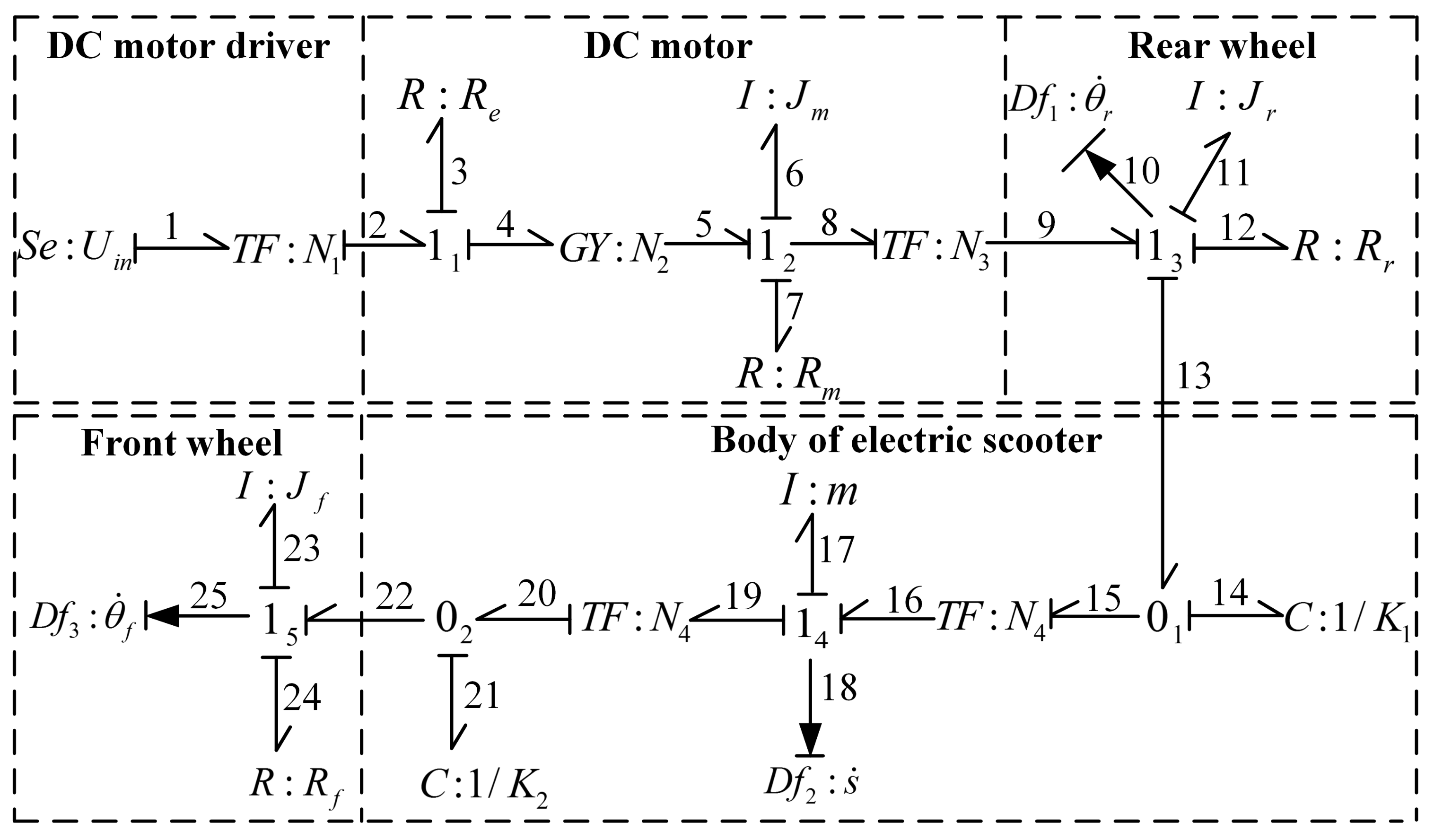
2.1. DBG Model of Electric Scooter

The structure diagram of the electric scooter is given in Figure 1, based on which its DBG model can be built, as shown in Figure 2. The DBG model of the electric scooter contains five parts, i.e., DC motor driver, DC motor, rear wheels, body, and front wheels. Descriptions of the main parameters of the model are summarized in

Table 1. Nomenclatures.

Parameter	Description
$U_{in}$	Input signal
$N_1$	Voltage-to-current ratio
$N_2$	Current-to-torque constant
$N_3$	Reduction ratio
$N_4$	Wheel radius
$K_1$, $K_2$	Transmission axes rigidity
m	Scooter mass
$R_e$	Electrical resistance
$R_{mv}$	Motor viscous friction coefficient
$R_{mc}$	Motor Coulomb friction torque
$J_m$	Motor inertia
$R_{rv}$	Rear wheel viscous friction coefficient
$R_{rc}$	Rear wheel Coulomb friction torque
$J_r$	Rear wheel inertia
$R_{fv}$	Front wheel viscous friction coefficient
$R_{fc}$	Front wheel Coulomb friction torque
$J_f$	Front wheel inertia

. In the DBG model of the electric scooter system, the mechanical friction $R_m$ of the DC motor consists of a viscous friction coefficient $R_{mv}$ and Coulomb friction torque $R_{mc}$. Similarly, the rear wheel friction $R_r$ contains a viscous friction coefficient $R_{rv}$ and Coulomb friction torque $R_{rc}$. The front wheel friction $R_f$ also contains a viscous friction coefficient $R_{fv}$ and Coulomb friction torque $R_{fc}$. Additionally, there are three flow sensors in the BG model: $D{f}_1:{\dot{\theta }}_r$ and $D{f}_3:{\dot{\theta }}_f$ are used to measure the angular velocities of rear wheels and front wheels, respectively, and $D{f}_2:\dot{s}$ is adopted to measure the line velocity of the electric scooter body.

2.2. FDI Method

Based on the DBG model in Figure 2, three modified analytical redundancy relations (MARRs) can be derived: (1)–(3). Differing from the traditional ARRs, MARRs is derived by introducing the efficiency factors to model the multiplicative faults of non-parametric components (including actuators and sensors).

$$\begin{array}{cc}\hfill {MARR}_1& =\frac{N_1·N_2}{N_3}·{\beta }_{U_{in}}·U_{in}-\frac{R_{mv}}{N_3^2}·\frac{d}{dt}\left(\frac{{\theta }_r}{{\beta }_{{\theta }_r}}\right)-\frac{R_{mc}}{N_3}·sign\left[\frac{d}{dt}\left(\frac{{\theta }_r}{{\beta }_{{\theta }_r}}\right)\right]\hfill \\ \hfill & -\frac{J_m}{N_3^2}·\frac{d^2}{d{t}^2}\left(\frac{{\theta }_r}{{\beta }_{{\theta }_r}}\right)-R_{rv}·\frac{d}{dt}\left(\frac{{\theta }_r}{{\beta }_{{\theta }_r}}\right)-R_{rc}·sign\left[\frac{d}{dt}\left(\frac{{\theta }_r}{{\beta }_{{\theta }_r}}\right)\right]\hfill \\ \hfill & -J_r·\frac{d^2}{d{t}^2}\left(\frac{{\theta }_r}{{\beta }_{{\theta }_r}}\right)-K_1·\left(\frac{{\theta }_r}{{\beta }_{\theta r}}-N_4·\frac{s}{{\beta }_s}\right)\hfill \end{array}$$

(1)

$$\begin{array}{cc}\hfill {MARR}_2& =K_1·N_4·\left(\frac{{\theta }_r}{{\beta }_{{\theta }_r}}-N_4·\frac{s}{{\beta }_s}\right)-m·\frac{d^2}{d{t}^2}\left(\frac{s}{{\beta }_s}\right)-K_2·N_4·\left(N_4·\frac{s}{{\beta }_s}-\frac{{\theta }_f}{{\beta }_{{\theta }_f}}\right)\hfill \end{array}$$

(2)

$$\begin{array}{cc}\hfill {MARR}_3& =K_2·\left(N_4·\frac{s}{{\beta }_s}-\frac{{\theta }_f}{{\beta }_{{\theta }_f}}\right)-R_{fv}·\frac{d}{dt}\left(\frac{{\theta }_f}{{\beta }_{{\theta }_f}}\right)-J_f·\frac{d^2}{d{t}^2}\left(\frac{{\theta }_f}{{\beta }_{{\theta }_f}}\right)\hfill \\ \hfill & -R_{fc}·sign\left[\frac{d}{dt}\left(\frac{{\theta }_f}{{\beta }_{{\theta }_f}}\right)\right]\hfill \end{array}$$

(3)

where ${\beta }_{U_{in}}$, ${\beta }_{{\theta }_r}$, ${\beta }_s$, and ${\beta }_{{\theta }_f}$ denote the efficiency factors of non-parametric components (i.e., $U_{in}$, ${\theta }_r$, s, and ${\theta }_f$).

If the residuals (numerical evaluations of MARRs) exceed the preset thresholds, the intermittent faults can be detected. The fault detection results can be represented by a binary coherence vector CV = $\left[c{v}_{1}c{v}_{2}c{v}_3\right],$ $c{v}_i\in \left\{0,1\right\},i=1,\dots ,3$, which indicates the consistency of residuals (zero for consistent and nonzero for inconsistent). To investigate the fault isolability, the fault signature matrix (FSM), which represents the cause–effect relationships between component faults and residuals, is given in

Table 2. FSM of electric scooter.

	${\mathit{r}}_1$	${\mathit{r}}_2$	${\mathit{r}}_3$	${\mathit{D}}_{\mathit{b}}$	${\mathit{I}}_{\mathit{b}}$
$U_{in}$	1	0	0	1	0
$R_{rv}$	1	0	0	1	0
${\beta }_{{\theta }_r}$	1	1	0	1	0
${\beta }_s$	1	1	1	1	0
${\beta }_{{\theta }_f}$	0	1	1	1	0
$R_{fc}$	0	0	1	1	0
$R_{fv}$	0	0	1	1	0

. If a nonzero CV is obtained from the fault detection process, the fault isolation procedure can be implemented by comparing the CV with the FSM. Then, a set of possible faults (SPF) can be determined.

3. Distributed Intermittent Fault Estimation

3.1. Parameterization of Intermittently Faulty Component

The intermittent fault estimation aims to identify the intermittent fault magnitude, with appearing and disappearing instants for possible faulty components in SPF. Thus, the value change in $\theta$ ($\theta$ represents the parameter or efficiency factor in Table 2) under intermittent faults in the time interval $t\in [t_s,t_e]$ can be described by the following function:

$$\begin{array}{cc}\hfill \theta \left(t,{\mathit{F}}_{\theta },{\mathit{\lambda }}_{\theta },{\mathit{\mu }}_{\theta }\right)& =F_{nom,\theta }·\epsilon \left(t\right)-\left(F_{nom,\theta }-F_{\theta }^1\right)·\epsilon \left(t-{\lambda }_{\theta }^1\right)+\left(F_{nom,\theta }-F_{\theta }^1\right)·\epsilon \left(t-{\mu }_{\theta }^1\right)\hfill \\ \hfill & -\cdots -\left(F_{nom,\theta }-F_{\theta }^p\right)·\epsilon \left(t-{\lambda }_{\theta }^p\right)+\left(F_{nom,\theta }-F_{\theta }^p\right)·\epsilon \left(t-{\mu }_{\theta }^p\right)\hfill \end{array}$$

(4)

where $\epsilon (\ast )$ is the unit step function, $F_{nom,\theta }$ is the nominal value of $\theta$, ${\mathit{F}}_{\theta }=[F_{\theta }^1{F}_{\theta }^2...F_{\theta }^p]$ is the fault magnitude vector, ${\mathit{\lambda }}_{\theta }=[{\lambda }_{\theta }^1{\lambda }_{\theta }^2...{\lambda }_{\theta }^p]$ is the fault appearing instant vector, ${\mathit{\mu }}_{\theta }=[{\mu }_{\theta }^1{\mu }_{\theta }^2...{\mu }_{\theta }^p]$ is the fault disappearing instant vector, $t_s\le {\lambda }_{\theta }^1<{\mu }_{\theta }^1<{\lambda }_{\theta }^2<...<{\lambda }_{\theta }^p<{\mu }_{\theta }^p\le t_e$. Thus, $\theta (\ast )$ is the parameterized function of the faulty component with three sets of variables (i.e., ${\mathit{F}}_{\theta },{\mathit{\lambda }}_{\theta }$, and ${\mathit{\mu }}_{\theta }$) to be identified. Based on (4), the value changes in all possible faulty components in SPF can be described by parameterization functions.

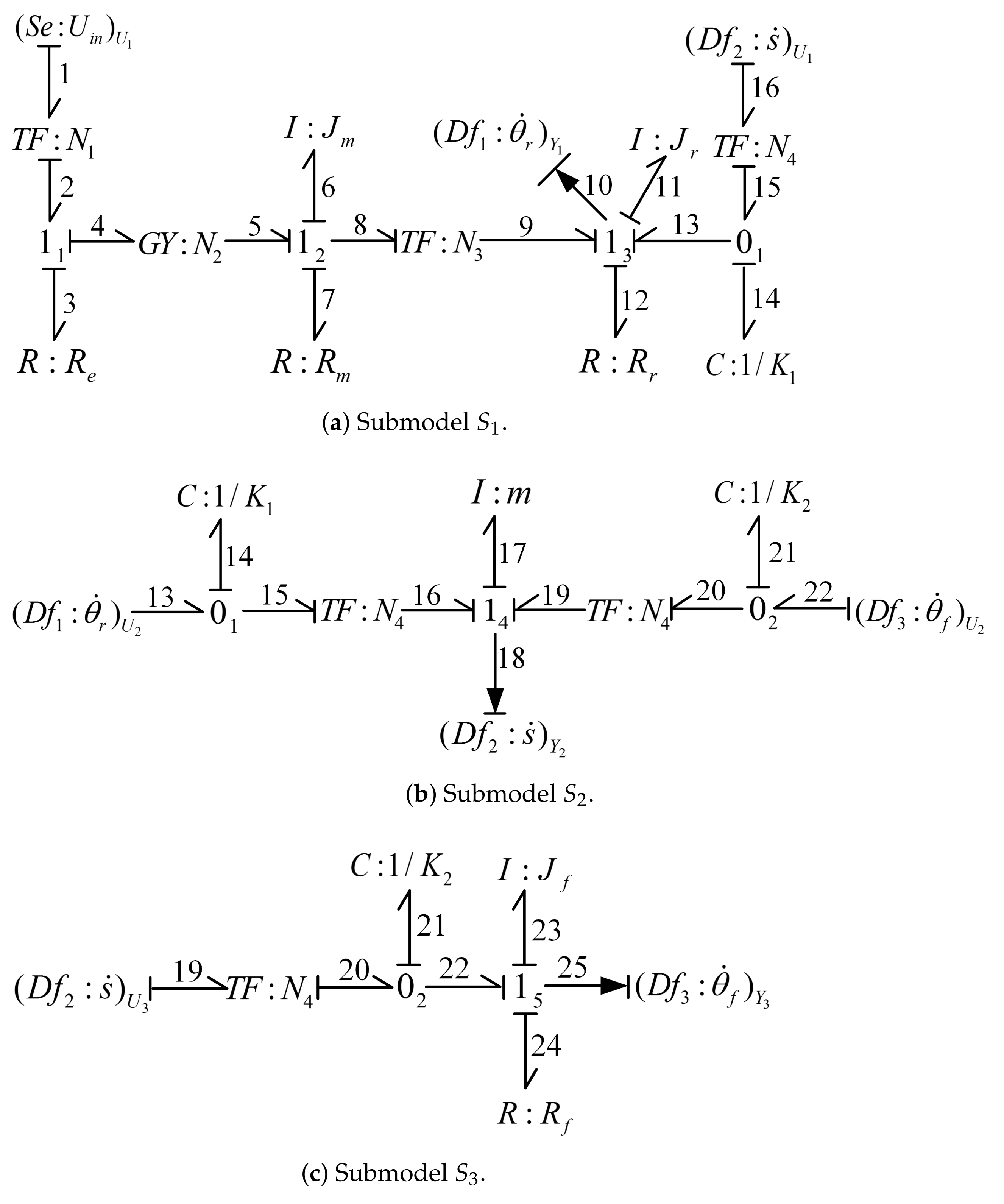
3.2. Construction of Submodels by Structural Model Decomposition

Since a large number of unknown variables need to be identified under the multiple intermittent faults condition (i.e., one has to identify the fault magnitude vector, fault-appearing instant vector and fault-disappearing instant vector for each fault candidate in SPF), there is a heavy computational burden if the centralized fault estimation method, based on the global model, is used. Therefore, the use of a distributed fault estimation technique is recommended to achieve better computational efficiency. The distributed fault estimation is accomplished based on the submodels that were decomposed from the global model using structural model decomposition [14,15]. For illustration, the global model and the submodel can be defined as follows.

Definition I: (Global model) A global model is represented by $G=(U,Y,\mathsf{\Theta })$, where U and Y are the sets of inputs and outputs of the global model, respectively, $\mathsf{\Theta }$ is the set of parameters and efficiency factors.

Definition II: (Submodel) The ith submodel is represented by $S_i=(U_i,Y_i,{\mathsf{\Theta }}_i)$, where $U_i\subset (U\cup Y)$ and $Y_i$ are the sets of local inputs and local output of the ith submodel, respectively, ${\mathsf{\Theta }}_i\subset \mathsf{\Theta }$ is the set of parameters and efficiency factors in the ith submodel.

Theoretically, the number of submodels is determined by the number of sensors in the global model. Therefore, three submodels, as shown in Figure 3, are built from the global DBG model of the electric scooter system. Based on Figure 3, the submodel MARRs can be derived as follows.

$$\begin{array}{cc}\hfill {MARR}_{S_1}& =\frac{N_1·N_2}{N_3}·{\beta }_{U_{in}}·{\left(U_{in}\right)}_{U_1}-\frac{R_{mv}}{N_3^2}·\frac{d}{dt}\left[\frac{{\left({\theta }_r\right)}_{Y_1}}{{\beta }_{{\theta }_r}}\right]-\frac{R_{mc}}{N_3}·sign\left\{\frac{d}{dt}\left[\frac{{\left({\theta }_r\right)}_{Y_1}}{{\beta }_{{\theta }_r}}\right]\right\}\hfill \\ \hfill & -\frac{J_m}{N_3^2}·\frac{d^2}{d{t}^2}\left[\frac{{\left({\theta }_r\right)}_{Y_1}}{{\beta }_{{\theta }_r}}\right]-R_{rc}·sign\left\{\frac{d}{dt}\left[\frac{{\left({\theta }_r\right)}_{Y_1}}{{\beta }_{{\theta }_r}}\right]\right\}-R_{rv}·\frac{d}{dt}\left[\frac{{\left({\theta }_r\right)}_{Y_1}}{{\beta }_{{\theta }_r}}\right]\hfill \\ \hfill & -J_r·\frac{d^2}{d{t}^2}\left[\frac{{\left({\theta }_r\right)}_{Y_1}}{{\beta }_{{\theta }_r}}\right]+K_1·\left[N_4·\frac{{\left(s\right)}_{U_1}}{{\beta }_s}-\frac{{\left({\theta }_r\right)}_{Y_1}}{{\beta }_{{\theta }_r}}\right]\hfill \end{array}$$

(5)

$$\begin{array}{cc}\hfill {MARR}_{S_2}& =K_1·N_4·\left[\frac{{\left({\theta }_r\right)}_{U_2}}{{\beta }_{{\theta }_r}}-N_4·\frac{{\left(s\right)}_{Y_2}}{{\beta }_s}\right]-m·\frac{d^2}{d{t}^2}\left[\frac{{\left(s\right)}_{Y_2}}{{\beta }_s}\right]\hfill \\ \hfill & +K_2·N_4·\left[\frac{{\left({\theta }_f\right)}_{U_2}}{{\beta }_{{\theta }_f}}-N_4·\frac{{\left(s\right)}_{Y_2}}{{\beta }_s}\right]\hfill \end{array}$$

(6)

$$\begin{array}{cc}\hfill {MARR}_{S_3}& =K_2·\left[N_4·\frac{{\left(s\right)}_{U_3}}{{\beta }_s}-\frac{{\left({\theta }_f\right)}_{Y_3}}{{\beta }_{\theta }}\right]-R_{fc}·sign\left\{\frac{d}{dt}\left[\frac{{\left({\theta }_f\right)}_{Y_3}}{{\beta }_{{\theta }_f}}\right]\right\}\hfill \\ \hfill & -R_{fv}·\frac{d}{dt}\left[\frac{{\left({\theta }_f\right)}_{Y_3}}{{\beta }_{{\theta }_f}}\right]-J_f·\frac{d^2}{d{t}^2}\left[\frac{{\left({\theta }_f\right)}_{Y_3}}{{\beta }_{{\theta }_f}}\right]\hfill \end{array}$$

(7)

In Figure 3 and (5)–(7), ${(\ast )}_{U_i}$ and ${(\ast )}_{Y_i}$ denote that ∗ is treated as the local input and output of the submodel $S_i$, $i=1,\dots ,3$, respectively. Note that the output (i.e., sensor measurement) in the global model may be treated as a local input or local output in different submodels. However, for the faulty sensor, regardless of the function it plays in the submodel (i.e., local input or local output), the efficiency factor should remain the same to ensure consistent detection results from different submodels.

In the electric scooter system, multiple intermittent faults are considered. Two typical cases are discussed in detail as follows.

Case I: Intermittent faults occur in ${\beta }_{U_{in}}$ and $R_{fc}$, CV = [1 0 1] and SPF = $\left\{{\beta }_{U_{in}},R_{rv},R_{fv},R_{fc}\right\}$ can be obtained by implementing the FDI procedure. Based on the SPF, ${\beta }_{U_{in}}$ and $R_{rv}$ are located at submodel $S_1$, while $R_{fv}$ and $R_{fc}$ are located at submodel $S_3$. Therefore, the $S_1$-based local estimator and the $S_3$-based local estimator can be implemented in parallel to identify ${\beta }_{U_{in}},R_{rv}$ and $R_{fv},R_{fc}$, respectively.

Case II: The intermittent fault occurs in ${\beta }_{{\theta }_r}$, CV = [1 1 0] and SPF = $\left\{{\beta }_{U_{in}},R_{rv},{\beta }_{{\theta }_r}\right\}$ are obtained. ${\beta }_{U_{in}}$ and $R_{rv}$ are located at submodel $S_1$, while ${\beta }_{{\theta }_r}$ exists in both submodels, $S_1$ and $S_2$. Since the submodel $S_1$ contains all possible faulty components in SPF, the $S_1$-based local estimator can be used to identify ${\beta }_{U_{in}},R_{rv}$, and ${\beta }_{{\theta }_r}$.

3.3. Distributed Fault Estimation via ACS Algorithm

Since the ${MARR}_{S_i}$ of the submodel $S_i$ is the function of $\theta$, and $\theta$ can be represented as the function of the unknown variables to be identified based on (4). The distributed fault estimation problem for submodel $S_i$ can be considered as the optimization problem using the following fitness function:

$$\begin{array}{c}\hfill F_{fit}=1/(\sum _{r=1}^R|{MARR}_{S_i,r}|+\rho )\end{array}$$

(8)

where R is the number of samples. The possible faults in an ${MARR}_{S_i}$ need to be represented by (4), such that the corresponding unknown variables can be obtained by the optimization algorithm, and $\rho$ is a small constant to avoid zero division.

After the fitness function of each submodel is obtained, the submodel-based local estimators that are affected by faults can be activated. ACS is utilized for fault parameter identification in the local estimators, while ACS is developed by introducing the adaptive step-size scaling factor into the standard Cuckoo search (CS). The CS, as a natural heuristic algorithm, is proposed to be inspired by brood parasitism and Levy flight (LF) foraging behaviors of cuckoos [29]. Suppose that $z_d^{l+1}$ and $z_d^l$ denote the positions of the lth and the $(l+1)$th generations of the cuckoo d, respectively. Then, the LF-based position updating formulation is expressed as

$$z_d^{l+1}=z_d^l+\alpha \otimes Levy(s,\gamma )$$

(9)

where $\alpha$ is the step-size scaling factor, ⊗ denotes the entry-wise multiplication, $Levy(s,\gamma )$ represents the LF random search path, and the random step-size obeys the Levy distribution as follows:

$$Levy\sim u=t^{-\gamma },1<\gamma \le 3$$

(10)

The Mantegna algorithm, which can achieve a symmetric Levy stable distribution, is usually an effective means of generating a random step-size that obeys the Levy distribution. Specifically, the step-size s is calculated via two variables with Gaussian distribution, as follows:

$$s=\frac{A}{{\left|B\right|}^{1/\gamma }},A\sim N(0,{\sigma }^2),B\sim N(0,1)$$

(11)

where

$$\sigma ={\left[\frac{\mathsf{\Gamma }(1+\gamma )}{\gamma \mathsf{\Gamma }\left(\right(1+\gamma )/2)}·\frac{sin(\pi \gamma /2)}{2^{(\gamma -1)/2}}\right]}^{1/\gamma }$$

(12)

The Levy index $\gamma =1.5$ and the step-size scaling factor $\alpha =1$ are default setups for the standard CS. However, the standard CS lacks the dynamical adaptability of search step-size, which may cause difficulties in algorithm convergence and lower estimation accuracy [30]. Therefore, the ACS is proposed to alleviate this problem, where the dynamic adaptive strategy of the step-size scaling factor based on (13) is introduced to the original CS. Using (13), the dynamic adaptive strategy is expressed by a nonlinear piece-wise function, where the larger $\alpha$ at the early searching stage helps the algorithm to converge to near the optimal solution quickly, while the smaller $\alpha$ at a later stage can achieve fine-tuning near the optimal solution.

$$\begin{array}{cc}\hfill & {\alpha }^l=\left\{\begin{array}{cc}{\alpha }_{max}\left[1-\frac{2e}{e^2-1}sinh{\left(\frac{l}{l_{max}}\right)}^2\right],\hfill & l<\frac{1}{3}{l}_{max}\hfill \\ {\alpha }_{min}+\left[1-\frac{2e}{e^2-1}sinh{\left(\frac{l}{l_{max}}\right)}^{\frac{1}{2}}\right],\hfill & \frac{1}{3}{l}_{max}\le l<\frac{2}{3}{l}_{max}\hfill \\ {\alpha }_{min},\hfill & l\ge \frac{2}{3}{l}_{max}\hfill \end{array}\right.\hfill \end{array}$$

(13)

where ${\alpha }_{max}$, ${\alpha }_{min}$, and ${\alpha }^l$ represent the maximum, the minimum and the lth generation step-size scaling factor of the algorithm, respectively. l is the current iteration number, and $l_{max}$ is the maximum number of iterations.

4. ACS-ELM Based Prognosis under Intermittent Fault

4.1. ELM Theory

When the value changes in intermittently faulty components are identified by ACS-based distributed fault estimation, the prognosis module can be activated to predict the RULs of intermittently faulty components. If the degradation model is predefined, the RUL of the faulty component can be successfully predicted using identification results, while the actual physical degradation model is usually unknown for most industrial applications. Therefore, neural networks, which can predict future behaviors based on historical data, have gradually become an important means of implementing RUL prediction. Among the various neural networks, ELM is a kind of single hidden-layer feedforward neural network, which possesses the advantages of fewer training parameters, a faster learning speed, and a stronger generalization ability [23,24,25,26,27]. When applying ELM to the prognosis of intermittently faulty components, the basic principle of ELM is introduced as follows.

Suppose that an arbitrary distinct sample set is $(X_i,$$Y_i)$, where $X_i={[x_{i1},x_{i2},\dots ,x_{in}]}^T\in R^n$ and $Y_i={[y_{i1},y_{i2},\dots ,y_{im}]}^T\in R^m$. The single hidden layer neural network with L hidden layer nodes can be expressed as

$$\sum _{i=1}^L{\mathit{\beta }}_{i}g(W_i·X_j+b_i)=o_j,j=1,\dots ,N$$

(14)

where $g(\ast )$ is the activation function, $W_i={[w_{i1},w_{i2},\dots ,w_{in}]}^T$ and ${\mathit{\beta }}_i={[{\beta }_{i1},{\beta }_{i2},\dots ,{\beta }_{im}]}^T$ denote input weight vector and output weight vector, respectively, $b_i$ is the bias of the ith hidden node, $W_i·X_j$ represents the inner product of $W_i$ and $X_j$. The learning goal of a single hidden-layer neural network is to minimize the output error, i.e., ${\sum }_{j=1}^N\left|\right|o_j-Y_j\left|\right|=0$. Thus, ${\mathit{\beta }}_i$, $W_i$, and $b_i$ exist, such that

$$\sum _{i=1}^L{\mathit{\beta }}_{i}g(W_i·X_j+b_i)=Y_j,j=1,\dots ,N$$

(15)

where input weight matrix, hidden layer bias vector, and input matrix can be expressed as $\mathbf{W}=[W_1{W}_2\dots W_L]$, $\mathit{b}=[b_1{b}_2\dots b_L]$, and $\mathbf{X}=[X_1{X}_2\dots X_N]$, respectively. Thus, (15) can also be represented by matrix form, as follows:

$$\begin{array}{cc}\hfill & \mathbf{H}(\mathbf{W},\mathit{b},\mathbf{X})\mathsf{\beta }=\mathbf{Y}\hfill \end{array}$$

(16)

where

$$\begin{array}{cc}\hfill & \mathbf{H}={\left[\begin{array}{ccc}g(W_1·X_1+b_1)& \cdots & g(W_L·X_1+b_L)\\ ⋮& \cdots & ⋮\\ g(W_1·X_N+b_1)& \cdots & g(W_L·X_N+b_L)\end{array}\right]}_{N\times L}\hfill \\ \hfill & \mathsf{\beta }={\left[\begin{array}{ccc}{\mathit{\beta }}_1^T& \cdots & {\mathit{\beta }}_L^T\end{array}\right]}_{L\times m}^T,\mathbf{Y}={\left[\begin{array}{ccc}{Y}_1^T& \cdots & Y_L^T\end{array}\right]}_{N\times m}^T\hfill \end{array}$$

(17)

Since the input weight matrix $\mathbf{W}$ and hidden layer bias matrix $\mathit{b}$ are randomly generated, the hidden layer output matrix $\mathbf{H}$ can be directly calculated based on (16). Therefore, the ELM aims to find the solution of a linear system $\mathbf{H}\mathsf{\beta }=\mathbf{Y}$, and the output weight $\widehat{\mathsf{\beta }}$ can be calculated as

$$\begin{array}{cc}\hfill \left|\right|\mathbf{H}\widehat{\mathsf{\beta }}-\mathbf{Y}\left|\right|& =min\left|\right|\mathbf{H}\mathsf{\beta }-\mathbf{Y}\left|\right|,\mathsf{\beta }\in R^{L\times m}\hfill \\ \hfill \widehat{\mathsf{\beta }}& ={\mathbf{H}}^{†}\mathbf{Y}\hfill \end{array}$$

(18)

where ${\mathbf{H}}^{†}$ is the Moore–Penrose generalized inverse of $\mathbf{H}$.

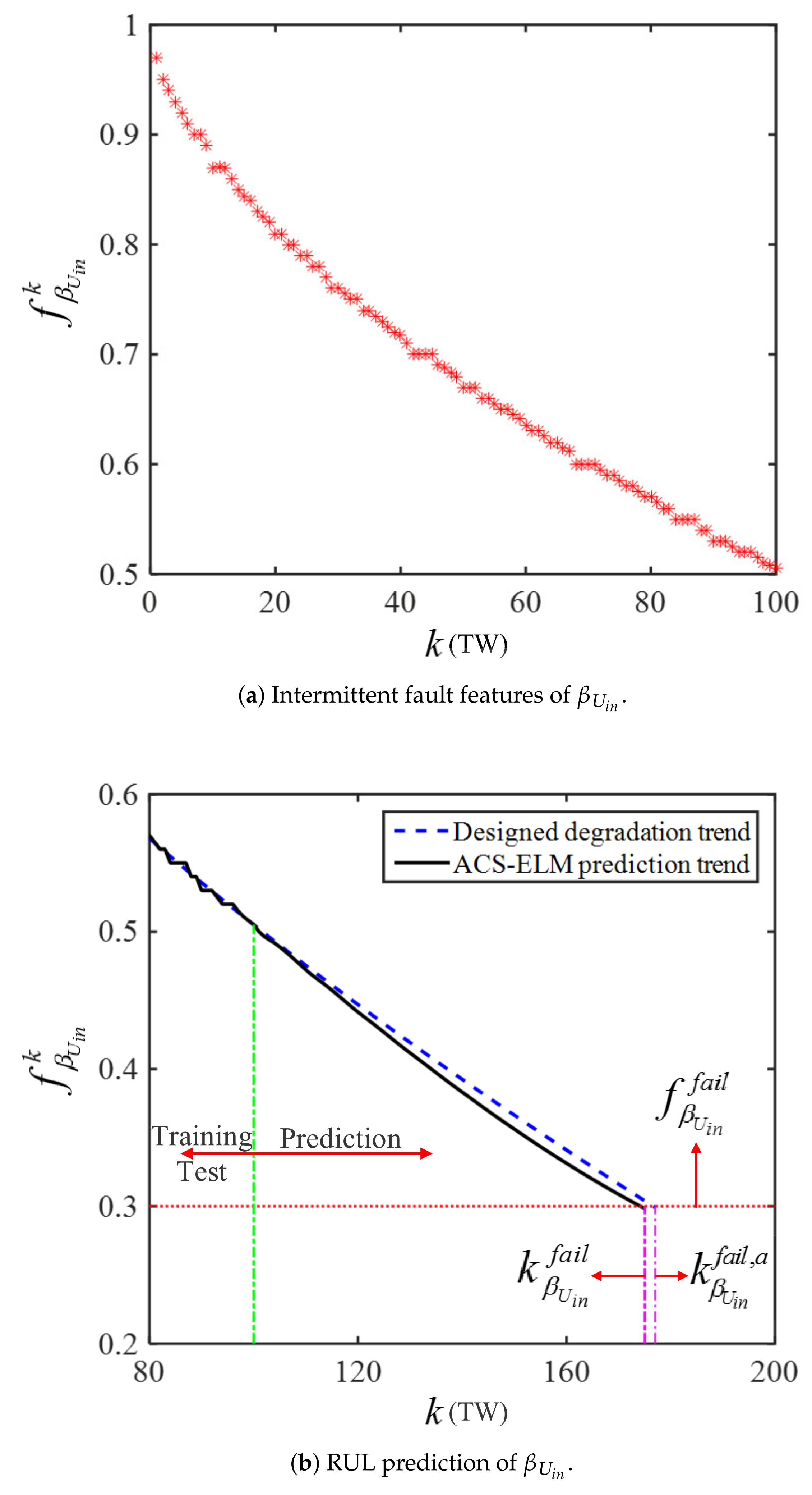
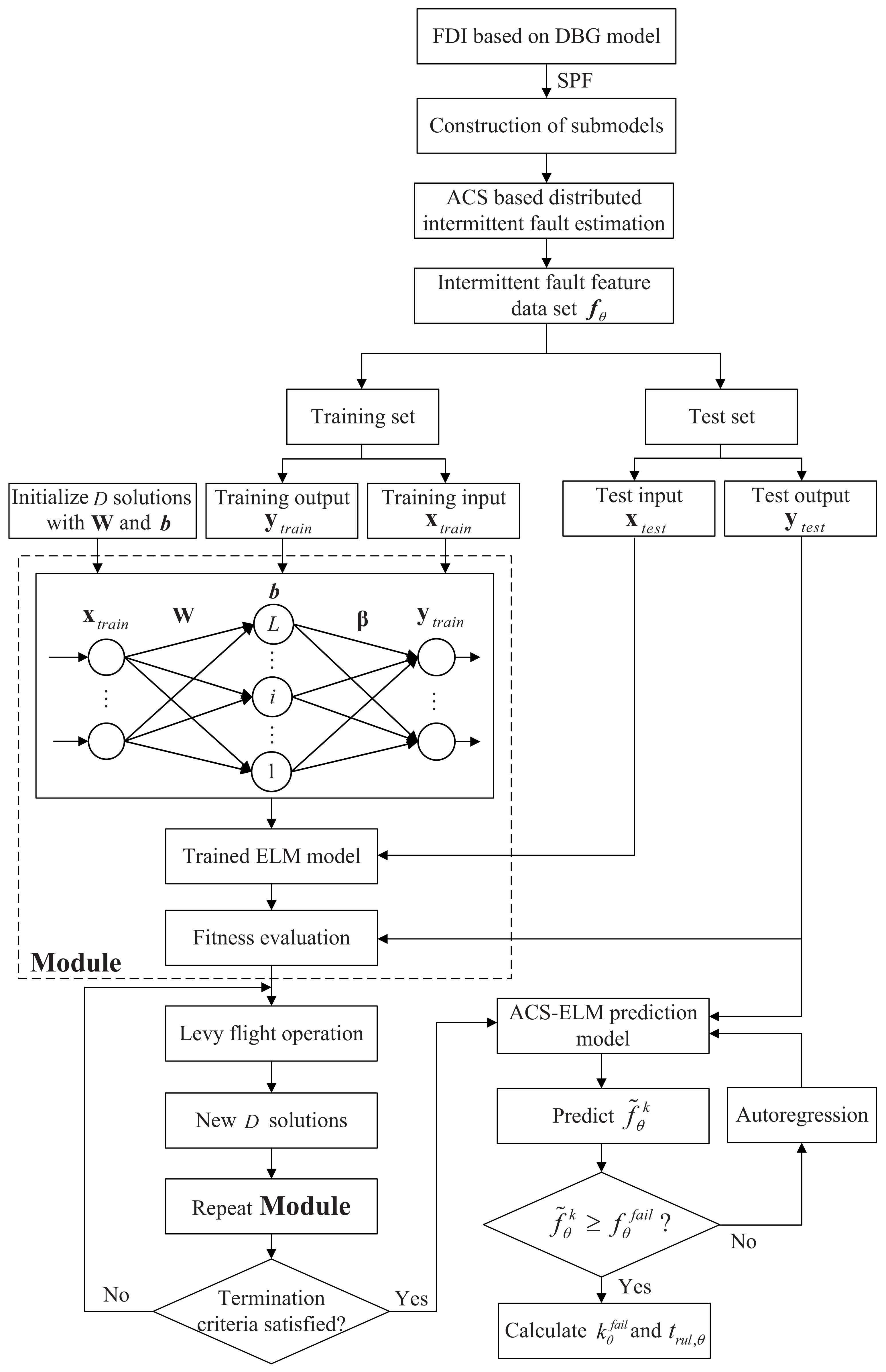
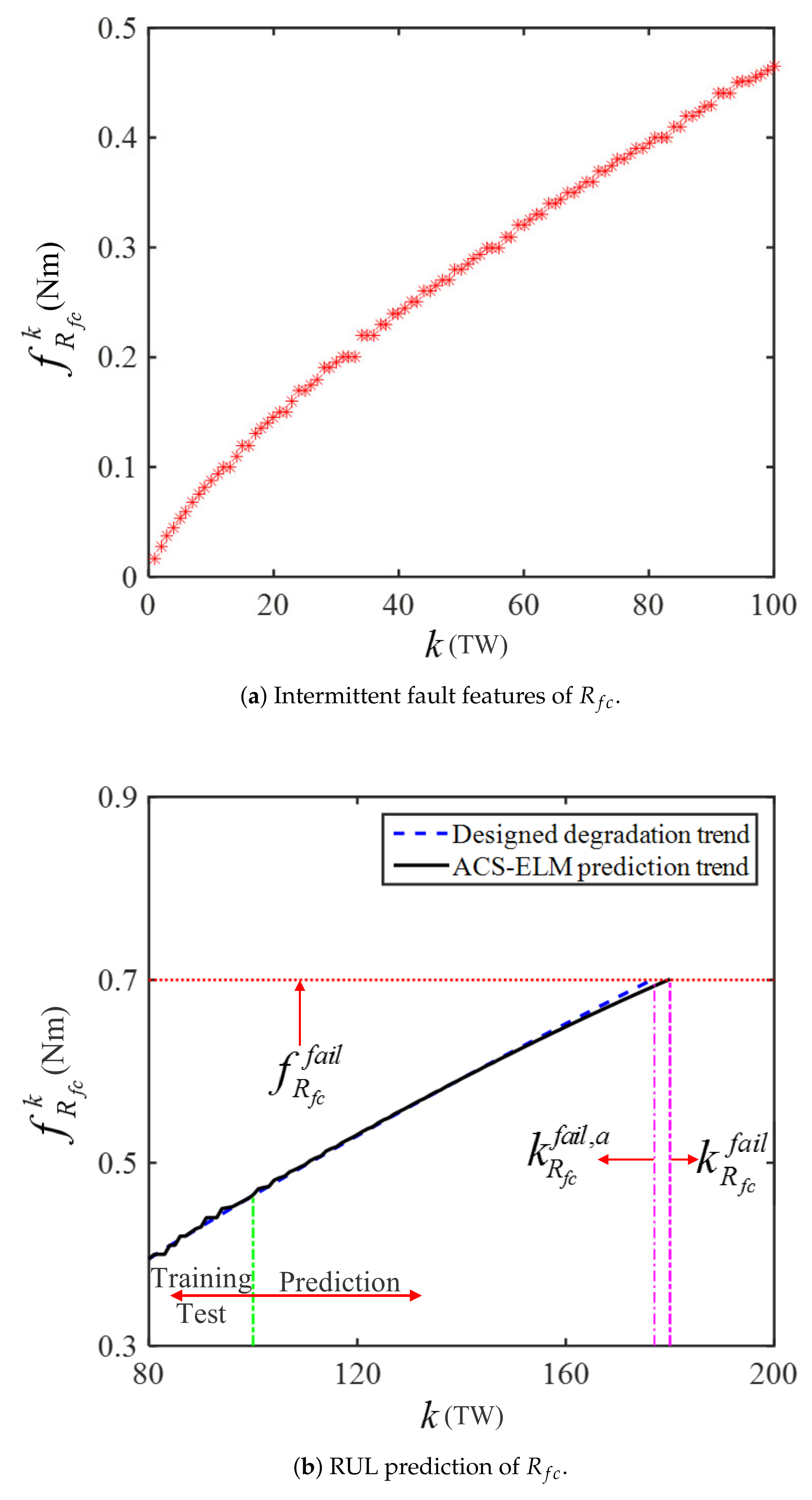
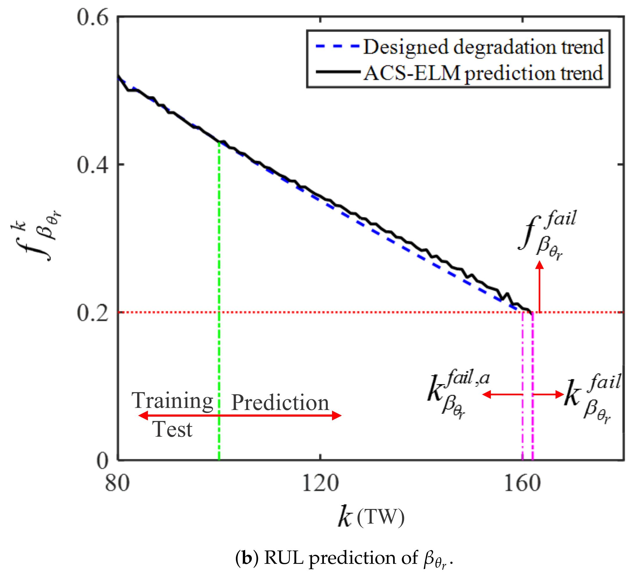
4.2. RUL Prediction for Intermittently Faulty Components Using ACS-ELM

Based on the ELM theory, the main steps of RUL prediction for intermittently faulty components using ACS-ELM approach can be described as follows.

Step 1: Construct an intermittent fault feature dataset.

To activate the ACS-ELM based prognoser, the intermittent fault features, which are used to build the training/test dataset, need to be constructed from the identification results. However, if the training/test set is determined via simply recording each intermittent fault magnitude as a fault feature, the intermittent fault features cannot be obtained at equal time intervals due to the discontinuity of intermittent faults and the randomness of fault appearance and disappearance, meaning that the one-step-ahead prediction of ELM cannot be properly implemented. To address this problem, the TW with a fixed length $L_{TW}$ is defined as the sampling length of the intermittent fault feature construction process, while the maximum fault magnitude in TW is treated as the intermittent fault feature. Therefore, the intermittent fault feature dataset can be expressed as follows:

$${\mathit{f}}_{\theta }=\left\{f_{\theta }^1,\dots ,f_{\theta }^k,\dots ,f_{\theta }^Q\right\},k=1,\dots ,Q,Q\in {\mathrm{N}}_{+}$$

(19)

$$\begin{array}{cc}\hfill f_{\theta }^k=& F_{nom,\theta }\pm max\left\{|F_{\theta }^{k,m}-F_{nom,\theta }|\right\},m=1,\dots ,M\hfill \end{array}$$

(20)

where Q is the number of intermittent fault features in the time interval $t\in [t_{d,\theta },t_{d,\theta }+Q·L_{TW}]$; $t_{d,\theta }$ is the instant at which the intermittent fault first occurs; $f_{\theta }^k$ represents the fault feature of $\theta$ in the kth TW; $F_{\theta }^{k,m}$ denotes the magnitude of the mth fault appearance in the kth TW for $\theta$; the sign “±” is determined by the relation between $F_{\theta }^{k,m}$ and $F_{nom,\theta }$; the sign is “+” when $F_{\theta }^{k,m}>F_{nom,\theta }$ and “−” otherwise; M is the number of fault appearances in the kth TW.

To obtain enough intermittent fault features to establish the ELM prediction model, the evolutionary trend of intermittent faults over a long period must be acknowledged. Therefore, the corresponding local estimators containing SPF are activated once every $L_{TW}$ after the first intermittent fault is detected. Then, the intermittent fault feature in this TW can be obtained according to (20). After that, the above process is repeated with $L_{TW}$ as the period until the intermittent fault feature dataset ${\mathit{f}}_{\theta }$ is determined, as shown in (19).

Step 2: Determine the input/output matrix and choose a training/test set.

When the intermittent fault feature dataset ${\mathit{f}}_{\theta }$ is obtained, as the ELM uses the one-step-ahead prediction strategy to implement RUL estimation, the first U data in ${\mathit{f}}_{\theta }$ are taken as the inputs and the following are treated as the output. Thus, the input matrix $\mathbf{x}$ and the output matrix $\mathbf{y}$ can be expressed as:

$$\begin{array}{c}\hfill \mathbf{x}={\left[\begin{array}{cccc}{f}_{\theta }^1& f_{\theta }^2& \cdots & f_{\theta }^U\\ f_{\theta }^2& f_{\theta }^3& \cdots & f_{\theta }^{U+1}\\ ⋮& ⋮& \ddots & ⋮\\ f_{\theta }^{Q-U}& f_{\theta }^{Q-U+1}& \cdots & f_{\theta }^{Q-1}\end{array}\right]}_{(Q-U)\times U},\mathbf{y}={\left[\begin{array}{c}{f}_{\theta }^{U+1}\\ f_{\theta }^{U+2}\\ ⋮\\ f_{\theta }^Q\end{array}\right]}_{(Q-U)\times 1}\end{array}$$

(21)

To train the ELM model for RUL prediction, the first V rows and the remaining $Q-U-V$ rows of $\mathbf{x}$ and $\mathbf{y}$ are treated as the training set $\left\{{\mathbf{x}}_{train},{\mathbf{y}}_{train}\right\}$ and test set $\left\{{\mathbf{x}}_{test},{\mathbf{y}}_{test}\right\}$, which can be represented as:

$$\begin{array}{c}\hfill {\mathbf{x}}_{train}={\left[\begin{array}{cccc}{f}_{\theta }^1& f_{\theta }^2& \cdots & f_{\theta }^U\\ f_{\theta }^2& f_{\theta }^3& \cdots & f_{\theta }^{U+1}\\ ⋮& ⋮& \ddots & ⋮\\ f_{\theta }^V& f_{\theta }^{V+1}& \cdots & f_{\theta }^{U+V-1}\end{array}\right]}_{V\times U},{\mathbf{y}}_{train}={\left[\begin{array}{c}{f}_{\theta }^{U+1}\\ f_{\theta }^{U+2}\\ ⋮\\ f_{\theta }^{U+V}\end{array}\right]}_{V\times 1}\end{array}$$

(22)

$$\begin{array}{c}\hfill {\mathbf{x}}_{test}={\left[\begin{array}{cccc}{f}_{\theta }^{V+1}& f_{\theta }^{V+2}& \cdots & f_{\theta }^{V+U}\\ f_{\theta }^{V+2}& f_{\theta }^{V+3}& \cdots & f_{\theta }^{V+U+1}\\ ⋮& ⋮& \ddots & ⋮\\ f_{\theta }^{Q-U}& f_{\theta }^{Q-U+1}& \cdots & f_{\theta }^{Q-1}\end{array}\right]}_{(Q-U-V)\times U},{\mathbf{y}}_{test}={\left[\begin{array}{c}{f}_{\theta }^{V+U+1}\\ f_{\theta }^{V+U+2}\\ ⋮\\ f_{\theta }^Q\end{array}\right]}_{(Q-U-V)\times 1}\end{array}$$

(23)

Step 3: Optimize the input weights and hidden layer biases using ACS.

To establish the canonical ELM model, the input weight matrix $\mathbf{W}$ and the hidden layer bias vector $\mathit{b}$ are randomly selected. However, the random selection of $\mathbf{W}$ and $\mathit{b}$ may lead to reductions in the generalization ability and prediction accuracy of the canonical ELM. To address the above problems, the ACS algorithm developed in Section 3.3 is adopted to optimize the input weights and hidden layer biases of ELM so that an optimal ELM model can be selected, i.e., ACS-ELM.

For ACS-ELM, a host nest $z_d$ (each host nest represents a feasible solution) in the population is composed of input weights and hidden layer biases. The fitness function is formulated by the mean square error of the ELM model output and the real output ${\mathbf{y}}_{test}$, which can be expressed as

$$G_{fit}=\frac{1}{Q-U-V}·\sum _{j=1}^{Q-U-V}{({\tilde{f}}_{\theta }^j-f_{\theta }^j)}^2$$

(24)

where ${\tilde{f}}_{\theta }^j$ is the actual output after ${\mathbf{x}}_{test}$ is substituted into the trained ELM model; $f_{\theta }^j$ is the desired output in the test set (i.e., ${\mathbf{y}}_{test}$). By minimizing the fitness function, the optimal solutions, including input weight matrix, hidden layer bias vector, and output weight matrix, can be determined, after which the ACS-ELM is obtained.

Step 4: Predict the RUL of intermittently faulty components.

When the ACS-ELM prediction model is determined, taking ${\mathbf{y}}_{test}$ as the initial input of the ACS-ELM prediction model, the one-step-ahead prediction procedure is implemented to predict the next intermittent fault feature until the predicted feature value ${\tilde{f}}_{\theta }^k$ exceeds the predefined threshold, i.e., $f_{\theta }^{fail}$. However, the RUL of the intermittently faulty component is predicted based on TW sampling, and the ACS-ELM-model-based prediction result refers to the $k_{\theta }^{fail}$th TW, in which the failure threshold $f_{\theta }^{fail}$ is exceeded. Therefore, the end-of-life (EOL) and RUL of the intermittently faulty component can be calculated as:

$$t_{eol,\theta }\in \left(t_{d,\theta }+(k_{\theta }^{fail}-1)·L_{TW},t_{d,\theta }+k_{\theta }^{fail}·L_{TW}\right]$$

(25)

$$\begin{array}{cc}\hfill & t_{rul,\theta }=t_{eol,\theta }-t_{d,\theta }-Q·L_{TW}\Rightarrow \hfill \\ \hfill & t_{rul,\theta }\in \left((k_{\theta }^{fail}-1-Q)·L_{TW},(k_{\theta }^{fail}-Q)·L_{TW}\right]\hfill \end{array}$$

(26)

Note that $\theta$ did not reach $f_{\theta }^{fail}$ at time $t_{d,\theta }+(k_{\theta }^{fail}-1)·L_{TW}$, and exceeded $f_{\theta }^{fail}$ at time $t_{d,\theta }+k_{\theta }^{fail}·L_{TW}$, while the exact intermittent fault condition cannot be determined in the time interval $t\in (t_{d,\theta }+(k_{\theta }^{fail}-1)·L_{TW},t_{d,\theta }+k_{\theta }^{fail}·L_{TW}]$ due to the stochasticity of intermittent faults. Therefore, the EOL and RUL of the intermittently faulty component are depicted by time intervals, as shown in (25) and (26), in which the magnitude of at least one fault will exceed the failure threshold rather than all faults.

Based on the above descriptions, the RUL prediction procedure for the intermittently faulty component using ACS-ELM is summarized in Figure 4.

5. Simulation and Experiment Results

To verify the effectiveness of the ACS-based distributed intermittent fault estimation method and the ACS-ELM-based intermittently faulty component prognosis method, a series of simulation and experiment analyses are carried out based on the electric scooter system in this section. The nominal values of the electric scooter system parameter are given in

Table 3. Nominal values of electric scooter parameter.

Nominal Parameter Values
$N_1$	0.2 A/V	$N_2$	1 Nm/A
$N_4$	1/0.105 m	$N_3$	1/18
$K_1$	10 Nm/rad	$K_2$	10 Nm/rad
$R_{mv}$	$1.72\times {10}^{-3}$ Nms/rad	$R_{mc}$	$5.63\times {10}^{-2}$ Nm
$R_{rv}$	$3.55\times {10}^{-3}$ Nms/rad	$R_{rc}$	$6.05\times {10}^{-2}$ Nm
$R_{fv}$	$1\times {10}^{-3}$ Nms/rad	$R_{fc}$	$1.86\times {10}^{-3}$ Nm
$J_m$	$5.03\times {10}^{-4}$ kgm${}^2$	$J_r$	$4.87\times {10}^{-3}$ kgm${}^2$
$J_f$	$6.97\times {10}^{-3}$ kgm${}^2$	$R_e$	1
m	20.7 kg

[28]. The sampling times are set as 0.02 s in both the simulation and experiment studies, and the intermittent fault feature sampling length (i.e., $L_{TW}$) is 10 s.

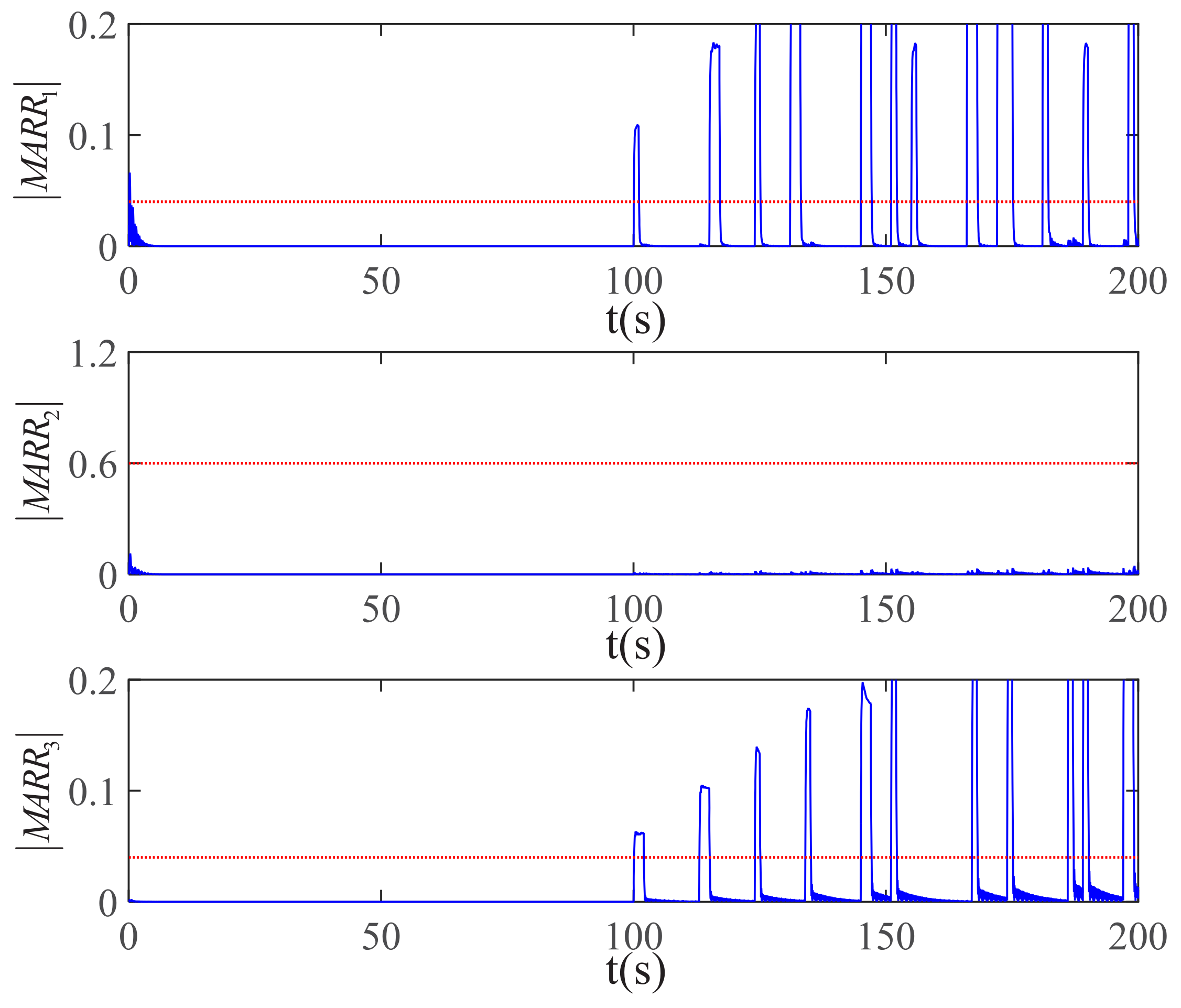
5.1. Simulation Study

In the simulation study, the fault scenario described in the Case I of Section 3.2 is considered, where intermittent faults occur in ${\beta }_{U_{in}}$ and $R_{fc}$. The simulation procedure is implemented in the MATLAB/Simulink environment, where the BG model of the electric scooter system is shown in Figure 2. The runtime of the electric scooter model in the simulation is 1100s; when the simulation runs to 100s, intermittent faults occur in ${\beta }_{U_{in}}$ and $R_{fc}$ simultaneously. The designed degradation processes of intermittent fault features of ${\beta }_{U_{in}}$ and $R_{fc}$ in TW are expressed as $f_{{\beta }_{U_{in}}}=1-0.03·k^{0.6088}$ and $f_{R_{fc}}=0.0167·k^{0.7221}+1.86\times {10}^{-3}$. Note that the intermittent faults of ${\beta }_{U_{in}}$ and $R_{fc}$ are both designed for the situation where the intermittent fault gradually deteriorates in magnitude, and possesses stochasticity in fault appearance and disappearance.

Firstly, the residual responses are shown in Figure 5, where dashed lines are thresholds and solid lines are residuals. The thresholds in the simulation process were chosen by observing the residual responses under normal simulation model conditions (i.e., 0.04 for $|{MARR}_1|$, 0.6 for $|{MARR}_2|$, and 0.04 for $|{MARR}_3|$). Only the residual responses of $t\in [0,200]$s are demonstrated in Figure 5 for easy observation, while the detection processes of the later 900s were similar to $t\in [0,200]$s, and were no longer on display. From Figure 6, it can be observed that ${MARR}_1$ and ${MARR}_3$ intermittently exceed their thresholds; accordingly, a CV can be determined as CV = [1 0 1], and the SPF was obtained by comparing CV with FSM, i.e., SPF = $\left\{{\beta }_{U_{in}},R_{rv},R_{fv},R_{fc}\right\}$.

Then, based on the descriptions of Case I of Section 3.2, $\left\{{\beta }_{U_{in}},R_{rv}\right\}$ and $\left\{R_{fv},R_{fc}\right\}$ can be estimated in parallel by a $S_1$-based local estimator and $S_3$-based local estimator. According to the construction method of the intermittent fault feature dataset, the $S_1$-based local estimator and the $S_3$-based local estimator are activated once every $L_{TW}=10$s to identify the magnitude and appearing and disappearing instants of each intermittent fault in the corresponding TW after the first intermittent fault is detected; then, the intermittent fault feature in each TW can be determined by (20). To obtain enough intermittent fault features to build the ACS-ELM prediction model, monitoring of the intermittent fault degradation process in the simulation lasts for 1000s (from 100s to 1100s), i.e., $Q=100$. Therefore, the distributed fault estimators need to be sequentially implemented 100 times to capture 100 intermittent fault features. From the estimation results, the actual values of $R_{rv}$ and $R_{fv}$ are consistent with their nominal values. Therefore, $R_{rv}$ and $R_{fv}$ can be excluded from the SPF, and it can be concluded that ${\beta }_{U_{in}}$ and $R_{fc}$ suffer from intermittent faults. To demonstrate the effectiveness and accuracy of the ACS-based distributed fault estimation approach, the identification results of the first two TWs are taken as examples for illustration. With these in mind, the distributed fault estimation results of ${\beta }_{U_{in}}$ and $R_{rv}$ of the first two TWs are shown in

Table 4. Comparison of designed values and estimated values.

(a) ${\beta }_{U_{in}}$
	TW${}_1$			TW${}_2$
${\beta }_{U_{in}}$	${\lambda }_{{\beta }_{U_{in}}}^1$(s)	${\mu }_{{\beta }_{U_{in}}}^1$(s)	$F_{{\beta }_{U_{in}}}^1$	${\lambda }_{{\beta }_{U_{in}}}^2$(s)	${\mu }_{{\beta }_{U_{in}}}^2$(s)	$F_{{\beta }_{U_{in}}}^2$
Designed value	100	101	0.97	115	117	0.95
Estimated value	100.0032	101.0023	0.9705	114.9978	117.0019	0.9509
(b) $R_{fc}$
	TW${}_1$			TW${}_2$
$R_{fc}$(Nm)	${\lambda }_{R_{fc}}^1$(s)	${\mu }_{R_{fc}}^1$(s)	$F_{R_{fc}}^1$	${\lambda }_{R_{fc}}^2$(s)	${\mu }_{R_{fc}}^2$(s)	$F_{R_{fc}}^2$
Designed value	100	102	1.8 $\times {10}^{-2}$	113	115	2.9 $\times {10}^{-2}$
Estimated value	100.0024	102.1015	1.806 $\times {10}^{-2}$	113.0012	114.9985	2.911 $\times {10}^{-2}$

. Table 4 shows the fault estimation results (including magnitude, appearing and disappearing instants of each intermittent fault in two TWs) versus the designed values. Thus, based on (20), $f_{{\beta }_{U_{in}}}^1=0.9705$, $f_{{\beta }_{U_{in}}}^2=0.9509$ and $f_{R_{fc}}^1=1.806\times {10}^{-2}$, $f_{R_{fc}}^2=2.911\times {10}^{-2}$ are determined. When the ACS-based distributed fault estimation process is terminated, all intermittent fault features are determined to form the intermittent fault feature dataset.

After that, the intermittent fault feature datasets of ${\beta }_{U_{in}}$ and $R_{fc}$, i.e., ${\mathit{f}}_{{\beta }_{U_{in}}}$ and ${\mathit{f}}_{R_{fc}}$, are depicted in Figure 6a and Figure 7a, respectively, where ${\mathit{f}}_{{\beta }_{U_{in}}}$ = $\left\{f_{{\beta }_{U_{in}}}^1,f_{{\beta }_{U_{in}}}^2,\dots ,f_{{\beta }_{U_{in}}}^{100}\right\}$ and ${\mathit{f}}_{R_{fc}}=\left\{f_{R_{fc}}^1,f_{R_{fc}}^2,\dots ,f_{R_{fc}}^{100}\right\}$ are both illustrated by 100 discrete points. With ${\mathit{f}}_{{\beta }_{U_{in}}}$ and ${\mathit{f}}_{R_{fc}}$, the ACS-ELM-based prognosis module introduced in Section 4.2 can be activated to predict the RULs of ${\beta }_{U_{in}}$ and $R_{fc}$. The ACS-ELM parameters are set as $Q=100$, $U=15$, $L=15$, $V=50$, and $g(\ast )=\frac{1}{1+exp(\ast )}$. The failure thresholds of ${\beta }_{U_{in}}$ and $R_{fc}$ are preset as $f_{{\beta }_{U_{in}}}^{fail}=0.3$ and $f_{R_{fc}}^{fail}=0.7$ Nm. The prediction results of ${\beta }_{U_{in}}$ and $R_{fc}$ using the ACS-ELM approach are illustrated in Figure 6b and Figure 7b. From Figure 6b, ${\beta }_{U_{in}}$ exceeds its failure threshold in the 175th TW, i.e., $k_{{\beta }_{U_{in}}}^{fail}=175$, thus the ranges of RUL of ${\beta }_{U_{in}}$ can be calculated as $t_{rul,{\beta }_{U_{in}}}\in ((k_{{\beta }_{U_{in}}}^{fail}-1-Q)·L_{TW},(k_{{\beta }_{U_{in}}}^{fail}-Q)·L_{TW}]=(740,750]$s based on (26). Similarly, it is clear that the prediction results of $R_{fc}$ are $k_{R_{fc}}^{fail}=180$ and $t_{rul,R_{fc}}\in (790,800]$s from Figure 7b.

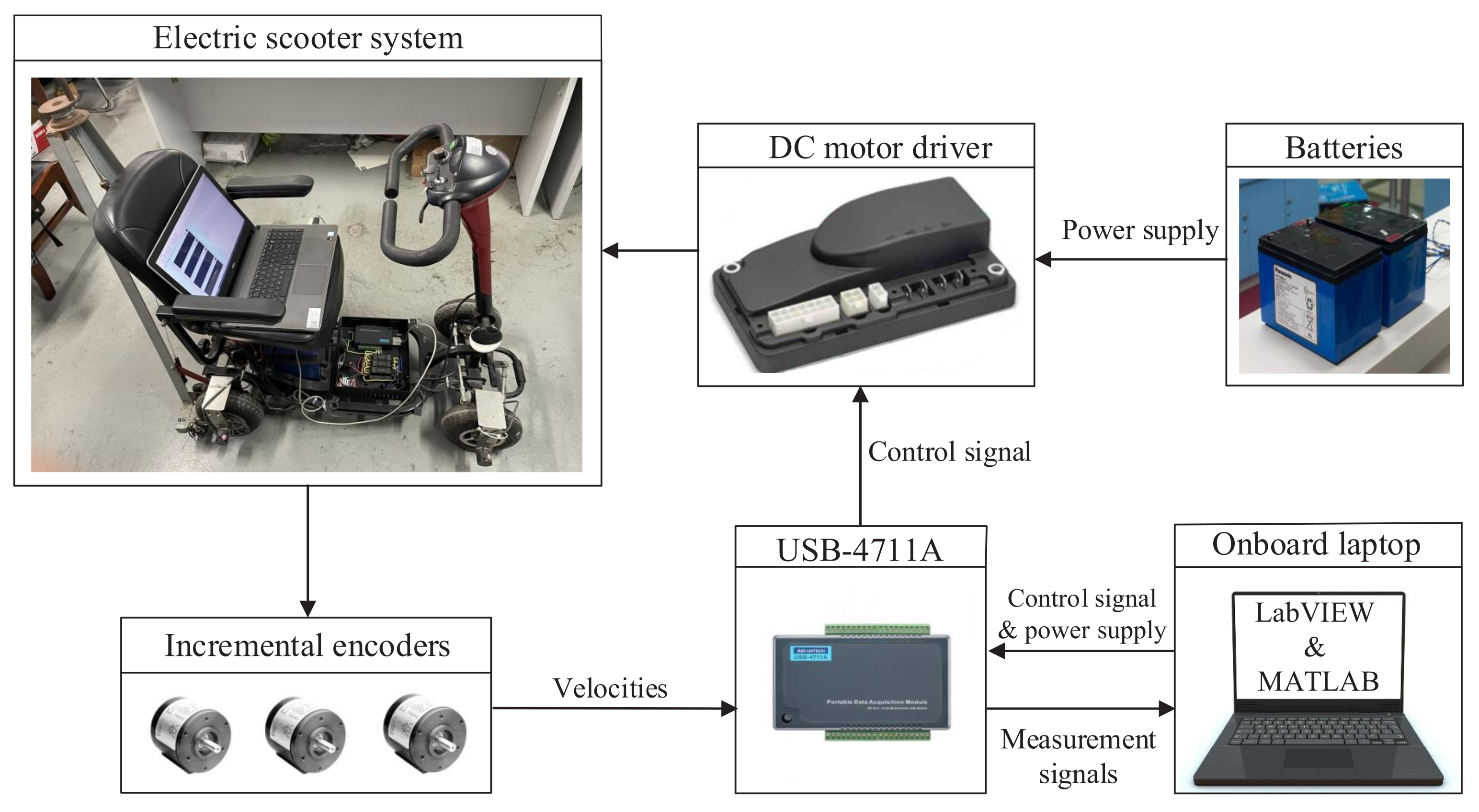
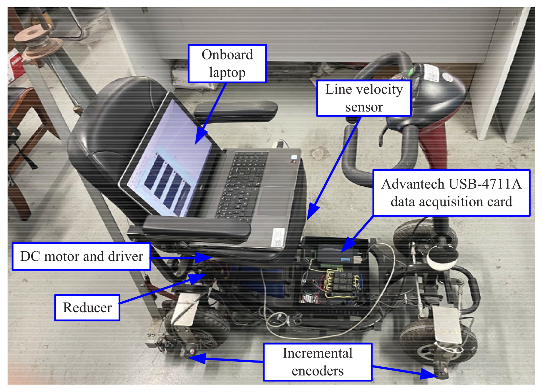
5.2. Experiment Study

To further investigate the performance of the proposed prognosis method under the experimental environment, the fault scenario described in the Case II of Section 3.2 was considered, where ${\theta }_r$ (i.e., ${\beta }_{{\theta }_r}$) suffers from intermittent faults. The designed degradation process of intermittent fault features of ${\beta }_{{\theta }_r}$ in TW was expressed as $f_{{\beta }_{{\theta }_r}}=1-0.02·k^{0.7268}$. A diagram of the experimental platform workflow is given in Figure 8. The lead–acid batteries (model: 12 V 20 AH lead–acid batteries) supplied power to the DC motor driver. The control signal to the DC motor driver (model: CRRTIS 1212-2201, nominal voltage 24 V, drive current 45 Amps, peak boost current 55 Amps, maximum boost duration 10 s) was provided by the USB data acquisition card (model: Advantech USB-4711A, USB 2.0 interface, 16 analog input channels, 12 bit resolution, sampling rate 150 kS/s), powered by the onboard laptop. The velocities of the electric scooter were measured by three incremental encoders (model: Omron E6B2-CWZ3E, resolution ratio 1000P/R, rated voltage 24 V). The onboard laptop provided voltage to the data acquisition card and sent an input signal to the motor driver. The FDI procedure of the electric scooter system was accomplished by the LabVIEW module, while distributed fault estimation and ACS-ELM based prognosis were conducted by introducing MATLAB script node into LabVIEW, based on which the co-simulation between MATLAB and LabVIEW could be implemented. The proposed methods were implemented in MATLAB R2015a and LabVIEW 2014 using an onboard laptop with an Intel Core i7-6500 2.6 GHz CPU with 8 GB memory and Microsoft Windows 7 Enterprise SP1 64-bit operating system.

Firstly, the fault detection results shown in Figure 9 indicate that the CV = [1 1 0] and SPF = $\left\{{\beta }_{U_{in}},R_{rv},{\beta }_{{\theta }_r}\right\}$. Note that a low-pass filter $\frac{5}{s+5}$ was used to deal with the measurement noises in the experiment and the thresholds of experiment had to be determined according to observations of the filtered residual responses of the actual system under healthy conditions (i.e., 0.2 for $|{MARR}_1|$, 3 for $|{MARR}_2|$, and 0.2 for $|{MARR}_3|$). Due to the description of Case II of Section 3.2, the submodel $S_1$ contained all possible faulty components in SPF, such that the $S_1$-based local estimator could be used to identify ${\beta }_{U_{in}},R_{rv}$, and ${\beta }_{{\theta }_r}$. Then, the ACS-based intermittent fault estimation for submodel $S_1$ was implemented; similar to the first fault scenario, the fault estimation results show that intermittent fault occured in ${\beta }_{{\theta }_r}$, while ${\beta }_{U_{in}}$ and $R_{rv}$ were fault-free. The intermittent fault feature dataset of ${\beta }_{{\theta }_r}$ was obtained according to (19) and (20), i.e., ${\mathit{f}}_{{\beta }_{{\theta }_r}}$ = $\left\{f_{{\beta }_{{\theta }_r}}^1,f_{{\beta }_{{\theta }_r}}^2,\dots ,f_{{\beta }_{{\theta }_r}}^{100}\right\}$, as illustrated in Figure 10a. Then, the parameters of ACS-ELM were set as $Q=100$, $U=15$, $L=15$, $V=50$, and $g(\ast )=\frac{1}{1+exp(\ast )}$. The obtained intermittent fault feature dataset ${\mathit{f}}_{{\beta }_{{\theta }_r}}$ was used to construct the ACS-ELM model, by which the RUL of ${\beta }_{{\theta }_r}$ could be predicted (the failure threshold of ${\beta }_{{\theta }_r}$ was preset as $f_{{\beta }_{{\theta }_r}}^{fail}=0.2$). Finally, the RUL prediction process is demonstrated in Figure 10b, and the prediction results were obtained as $k_{{\beta }_{{\theta }_r}}^{fail}=162$ and $t_{rul,{\beta }_{{\theta }_r}}\in (610,620]$s.

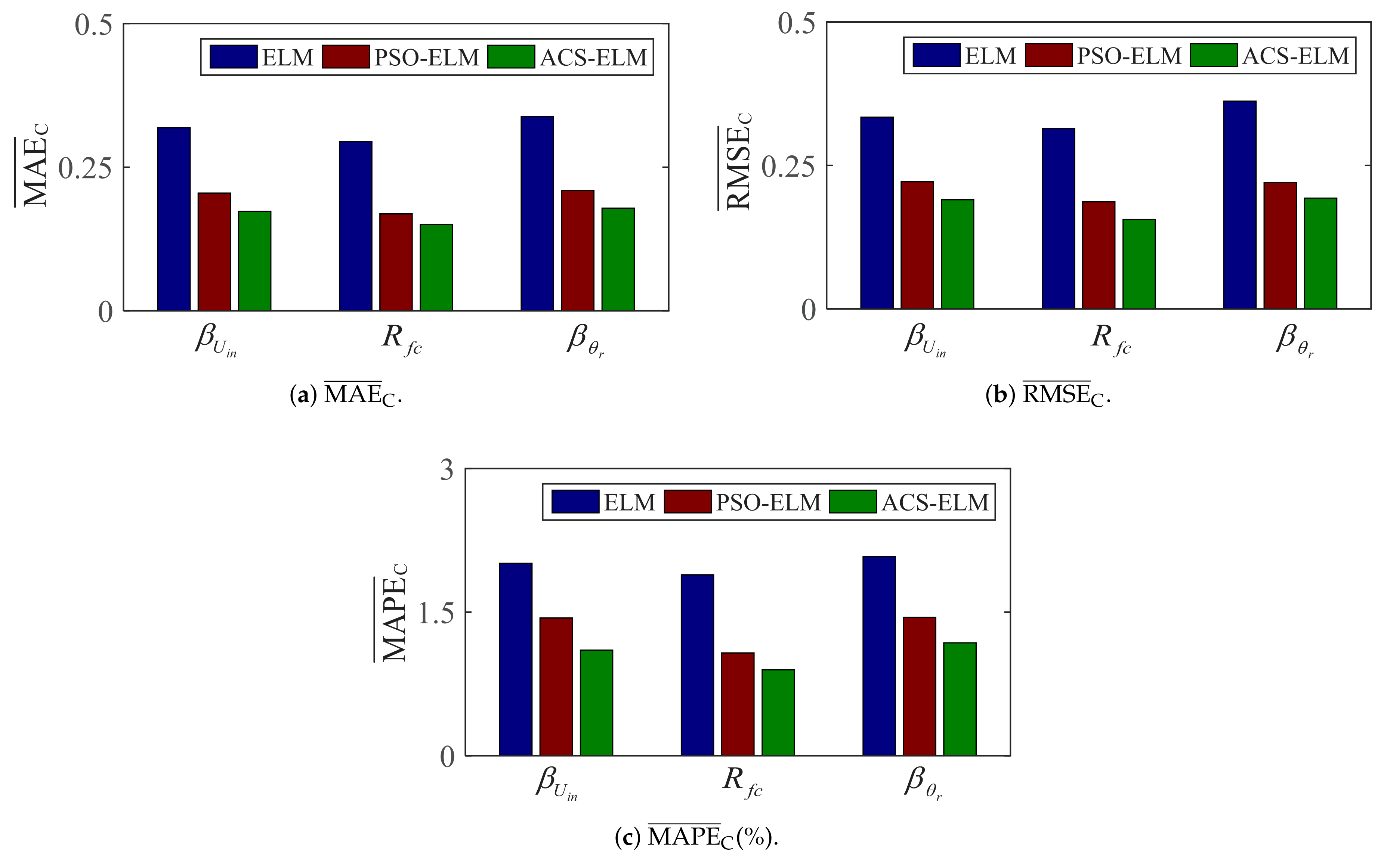
5.3. Analysis and Comparison

To evaluate the RUL prediction accuracy of ACS-ELM approach, three metrics, including mean absolute error (MAE), root means square error (RMSE), and mean absolute percentage error (MAPE), are adopted, which can be computed as

$$\mathrm{MAE}=\frac{1}{k_{\theta }^{fail}-Q}·\sum _{k=Q+1}^{k_{\theta }^{fail}}|{\widehat{f}}_{\theta }^k-f_{\theta }^{k,a}|$$

(27)

$$\mathrm{RMSE}=\sqrt{\frac{1}{k_{\theta }^{fail}-Q}·\sum _{k=Q+1}^{k_{\theta }^{fail}}|{\widehat{f}}_{\theta }^k-f_{\theta }^{k,a}{|}^2}$$

(28)

$$\mathrm{MAPE}=\frac{100\%}{k_{\theta }^{fail}-Q}·\sum _{k=Q+1}^{k_{\theta }^{fail}}\left|\frac{{\widehat{f}}_{\theta }^k-f_{\theta }^{k,a}}{f_{\theta }^{k,a}}\right|$$

(29)

where ${\widehat{f}}_{\theta }^k$ denotes the predicted intermittent fault feature in the kth TW for $\theta$; $f_{\theta }^{k,a}$ represents the designed intermittent fault feature in the kth TW according to the pre-designed degradation process of intermittent fault features for $\theta$.

According to the designed intermittent fault feature degradation processes of ${\beta }_{U_{in}}$, $R_{fc}$, and ${\beta }_{\theta r}$, i.e., $f_{{\beta }_{U_{in}}}=1-0.03·k^{0.6088}$, $f_{R_{fc}}=0.0167·k^{0.7221}+1.86\times {10}^{-3}$, and $f_{{\beta }_{{\theta }_r}}=1-0.02·k^{0.7268}$, the designed fault degradation trends of ${\beta }_{U_{in}}$, $R_{fc}$ and ${\beta }_{{\theta }_r}$ are depicted in Figure 6b, Figure 7b and Figure 10b, respectively. The evaluation metrics of the ACS-ELM-based RUL prediction results of the simulation and experiment are summarized in

Table 5. RUL prediction result evaluation of ACS-ELM.

	MAE	RMSE	MAPE(%)
${\beta }_{U_{in}}$	0.0071	0.0076	1.8773
$R_{fc}$	0.0022	0.0031	0.3630
${\beta }_{\theta r}$	0.0074	0.0084	2.6825

. Table 5 shows that the ACS-ELM-based prognosis for intermittently faulty components is accurate for both simulations and experiments.

Finally, a comparison study was conducted with traditional ELM and PSO-ELM [27] to validate the superiority of the proposed ACS-ELM-based prognosis method. To make a fair comparison, all approaches were tested on the same simulation or experiment data. Additionally, the population size, maximum iterations and search spaces of parameters for three algorithms were the same. Each approach used 30 independent tests (i.e., simulation for ${\beta }_{U_{in}}$ and $R_{fc}$, experiment for ${\beta }_{{\theta }_r}$). The mean value of MAE (i.e., $\overline{\mathrm{MAE}}$), obtained from 30 tests, was taken as the comparison index of algorithm performance, as were the mean values of RMSE and MAPE (i.e., $\overline{\mathrm{RMSE}}$ and $\overline{\mathrm{MAPE}}$). The comparison results of ELM, PSO-ELM, and ACS-ELM are summarized in

Table 6. Comparison of RUL prediction performance.

	Algorithm	$\overline{\mathbf{MAE}}$	$\overline{\mathbf{RMSE}}$	$\overline{\mathbf{MAPE}}$(%)
${\beta }_{U_{in}}$	ELM	0.0324	0.0373	8.1226
	PSO-ELM	0.0086	0.0109	2.9753
	ACS-ELM	0.0052	0.0069	1.3394
$R_{fc}$	ELM	0.0255	0.0312	6.7490
	PSO-ELM	0.0048	0.0065	1.2562
	ACS-ELM	0.0034	0.0038	0.7221
${\beta }_{\theta r}$	ELM	0.0387	0.0475	8.9917
	PSO-ELM	0.0092	0.0107	3.0169
	ACS-ELM	0.0057	0.0072	1.6385

. Meanwhile, the comparison results of the RUL prediction performance for different algorithms are depicted in Figure 11, where the cube roots of $\overline{\mathrm{MAE}}$, $\overline{\mathrm{RMSE}}$, and $\overline{\mathrm{MAPE}}$ (i.e., ${\overline{\mathrm{MAE}}}_{\mathrm{C}}$, ${\overline{\mathrm{RMSE}}}_{\mathrm{C}}$, and ${\overline{\mathrm{MAPE}}}_{\mathrm{C}}$) are calculated and illustrated in Figure 11 for observation. According to Table 6, compared with the standard ELM and PSO-ELM, the average prediction evaluation indexes (i.e., MAE, RMSE, and MAPE, respectively) in 30 trials of ACS-ELM were reduced by 83.95%, 81.50%, 83.51% (ELM compared to ACS-ELM) and 39.53%, 36.70%, 54.98% (PSO-ELM compared to ACS-ELM) for ${\beta }_{U_{in}}$, 86.67%, 87.82%, 89.45% and 29.17%, 41.54%, 42.52% for $R_{fc}$, 85.27%, 84.84%, 81.78% and 38.04%, 32.71%, 45.69% for ${\beta }_{{\theta }_r}$. It can be concluded that ACS-ELM performs better than traditional ELM and PSO-ELM in terms of RUL prediction under intermittent faults.

6. Conclusions

In this paper, an ACS-ELM-based prognosis method is developed for an electric scooter system with intermittent faults. The FDI framework helps to find possible faulty components. Based on the model’s structural decomposition and ACS algorithm, distributed fault estimation was implemented to identify the magnitude and the appearing and disappearing instants of each intermittent fault for faulty components. For the prognosis of intermittently faulty components, ACS-ELM was proposed to model the degradation process of intermittent fault features and predict the RUL of intermittently faulty components. A series of simulation and experiment results verified the effectiveness of the proposed methods. Through experiment and comparison studies, it is concluded that the ACS-ELM-based RUL prediction results of intermittently faulty components are accurate, and the ACS-ELM performs better than traditional ELM and PSO-ELM for prognosis under intermittent faults.

This work provides an effective method for the RUL prediction of intermittently faulty components under the condition of unavailable degradation models. Several challenging issues still need to be addressed. Future research directions will focus on the following two aspects. First, this work only considers the RUL prediction method of the intermittent fault magnitude degradation process based on ACS-ELM, while intermittent fault degradation can also be reflected in terms of duration. It is necessary to apply the proposed method to RUL predictions of the intermittent fault duration degradation process. Secondly, as the system working conditions (road conditions, system input, system mode, etc.) often change in practice, RUL predictions of intermittent faults under variations in system working conditions should be considered in future work.

References

1. Stoll, J.T.; Schanz, K.; Pott, A. Mechatronic control system for a compliant and precise pneumatic rotary drive unit. Actuators 2020, 9, 1. [Google Scholar] [CrossRef] [Green Version]
2. Zhang, J.; Wang, H.; Zheng, J.; Cao, Z.; Man, Z.; Yu, M.; Chen, L. Adaptive sliding mode-based lateral stability control of steer-by-wire vehicles with experimental validations. IEEE Trans. Veh. Technol. 2020, 69, 9589–9600. [Google Scholar] [CrossRef]
3. Aguzzi, J.; Costa, C.; Calisti, M.; Funari, V.; Stefanni, S.; Danovaro, R.; Gomes, H.I.; Vecchi, F.; Dartnell, L.R.; Weiss, P.; et al. Research trends and future perspectives in marine biomimicking robotics. Sensors 2021, 21, 3778. [Google Scholar] [CrossRef] [PubMed]
4. Shi, Y.; Shen, C.; Fang, H.; Li, H. Advanced control in marine mechatronic systems: A survey. IEEE/ASME Trans. Mechatron. 2017, 22, 1121–1131. [Google Scholar] [CrossRef]
5. Zhang, J.; Wang, H.; Ma, M.; Yu, M.; Yazdani, A.; Chen, L. Active front steering-based electronic stability control for steer-by-wire vehicles via terminal sliding mode and extreme learning machine. IEEE Trans. Veh. Technol. 2020, 69, 14713–14726. [Google Scholar] [CrossRef]
6. Cai, B.; Zhao, Y.; Liu, H.; Xie, M. A data-driven fault diagnosis methodology in three-phase inverters for PMSM drive systems. IEEE Trans. Power Electron. 2017, 32, 5590–5600. [Google Scholar] [CrossRef]
7. Zhang, J.; Yao, H.; Rizzoni, G. Fault diagnosis for electric drive systems of electrified vehicles based on structural analysis. IEEE Trans. Veh. Technol. 2017, 66, 1027–1039. [Google Scholar] [CrossRef]
8. Wang, X.; Wang, Z.; Xu, Z.; Cheng, M.; Wang, W.; Hu, Y. Comprehensive diagnosis and tolerance strategies for electrical faults and sensor faults in dual three-phase PMSM drives. IEEE Trans. Power Electron. 2019, 34, 6669–6684. [Google Scholar] [CrossRef]
9. Sundstrom, C.; Frisk, E.; Nielsen, L. Selecting and utilizing sequential residual generators in FDI applied to hybrid vehicles. IEEE Trans. Syst. Man Cybern. Syst. 2014, 44, 172–185. [Google Scholar] [CrossRef] [Green Version]
10. Yaramasu, M.; Cao, A.; Liu, G.; Wu, B. Aircraft electric system intermittent arc fault detection and location. IEEE Trans. Aerosp. Electron. Syst. 2015, 51, 45–51. [Google Scholar] [CrossRef]
11. Yan, R.; He, X.; Wang, Z.; Zhou, D. Detection, isolation and diagnosability analysis of intermittent faults in stochastic systems. Int. J. Control 2018, 9, 480–494. [Google Scholar] [CrossRef]
12. Obeid, N.H.; Battiston, A.; Boileau, T.; Nahid-Mobarakeh, B. Early intermittent interturn fault detection and localization for a permanent magnet synchronous motor of electrical vehicles using wavelet transform. IEEE Trans. Transport. Electrific. 2017, 3, 694–702. [Google Scholar] [CrossRef]
13. Arogeti, S.A.; Wang, D.; Low, C.B.; Yu, M. Fault detection isolation and estimation in a vehicle steering system. IEEE Trans. Ind. Electron. 2012, 59, 4810–4820. [Google Scholar] [CrossRef]
14. Bregon, A.; Daigle, M.J.; Roychoudhury, I.; Biswas, G.; Koutsoukos, X.; Pulido, B. An event-based distributed diagnosis framework using structural model decomposition. Artif. Intell. 2014, 210, 1–35. [Google Scholar] [CrossRef]
15. Daigle, M.J.; Bregon, A.; Roychoudhury, I. Distributed prognostics based on structural model decomposition. IEEE Trans. Reliab. 2014, 63, 495–510. [Google Scholar] [CrossRef] [Green Version]
16. Yu, M.; Lu, H.; Wang, H.; Xiao, C.; Lan, D.; Chen, J. Computational intelligence-based prognosis for hybrid mechatronic system using improved wiener process. Actuators 2021, 10, 213. [Google Scholar] [CrossRef]
17. Nguyen, V.; Seshadrinath, J.; Wang, D.; Nadarajan, S.; Vaiyapuri, V. Model-based diagnosis and RUL estimation of induction machines under interturn fault. IEEE Trans. Ind. Appl. 2017, 53, 2690–2701. [Google Scholar] [CrossRef]
18. Yu, M.; Wang, D. Model-based health monitoring for a vehicle steering system with multiple faults of unknown types. IEEE Trans. Ind. Electron. 2014, 61, 3574–3586. [Google Scholar]
19. Yu, M.; Xia, H.; He, Y.; Wang, H.; Jiang, C.; Chen, S.; Li, M.; Xu, J. Scheduled health monitoring of hybrid systems with multiple distinct faults. IEEE Trans. Ind. Electron. 2017, 64, 1517–1528. [Google Scholar] [CrossRef]
20. Lei, Y.; Li, N.; Gontarz, S.; Lin, J.; Radkowski, S.; Dybala, J. A model-based method for remaining useful life prediction of machinery. IEEE Trans. Reliab. 2016, 5, 1314–1326. [Google Scholar] [CrossRef]
21. Liu, R.; Yang, B.; Hauptmann, A.G. Simultaneous bearing fault recognition and remaining useful life prediction using joint-loss convolutional neural network. IEEE Trans. Ind. Inform. 2020, 16, 87–96. [Google Scholar] [CrossRef]
22. Xiao, L.; Duan, F.; Tang, J.; Abbott, D. A noise-boosted remaining useful life prediction method for rotating machines under different conditions. IEEE Trans. Instrum. Meas. 2021, 70, 1–12. [Google Scholar]
23. Huang, G.; Zhu, Q.; Siew, C. Extreme learning machine: Theory and applications. Neurocomputing 2006, 70, 489–501. [Google Scholar] [CrossRef]
24. Song, J.; Dong, F.; Zhao, J.; Wang, H.; He, Z.; Wang, L. An efficient multiobjective design optimization method for a PMSLM based on an extreme learning machine. IEEE Trans. Ind. Electron. 2019, 66, 1001–1011. [Google Scholar] [CrossRef]
25. Skordilis, E.; Moghaddass, R. A double hybrid state-space model for real-time sensor-driven monitoring of deteriorating systems. IEEE Trans. Autom. Sci. Eng. 2020, 17, 72–87. [Google Scholar] [CrossRef]
26. Lu, F.; Wu, J.; Huang, J.; Qiu, X. Aircraft engine degradation prognostics based on logistic regression and novel OS-ELM algorithm. Aerosp. Sci. Technol. 2019, 84, 661–671. [Google Scholar] [CrossRef]
27. Zeng, N.; Zhang, H.; Liu, W.; Liang, J.; Alsaadi, F.E. A switching delayed PSO optimized extreme learning machine for short-term load forecasting. Neurocomputing 2017, 240, 175–182. [Google Scholar] [CrossRef]
28. Yu, M.; Lu, H.; Wang, H.; Xiao, C.; Lan, D. Compound fault diagnosis and sequential prognosis for electric scooter with uncertainties. Actuators 2020, 9, 128. [Google Scholar] [CrossRef]
29. Gandomi, A.H.; Yang, X.; Alavi, A.H. Cuckoo search algorithm: A metaheuristic approach to solve structural optimization problems. Eng. Comput. 2013, 29, 17–35. [Google Scholar] [CrossRef]
30. Wang, Q.; Chai, M.; Liu, H.; Tang, T. Optimized control of virtual coupling at junctions: A cooperative game-based approach. Actuators 2021, 10, 207. [Google Scholar] [CrossRef]
Figure 1. Structure diagram of electric scooter.
Actuators 10 00283 g001
Figure 2. DBG model of electric scooter.
Actuators 10 00283 g002
Figure 3. Submodels of electric scooter.
Actuators 10 00283 g003
Figure 4. The framework of ACS-ELM based prognosis under intermittent fault.
Actuators 10 00283 g004
Figure 5. Residual responses under β U i n and R f c faults.
Actuators 10 00283 g005
Figure 6. Estimation and prediction results of β U i n .
Actuators 10 00283 g006
Figure 7. Estimation and prediction results of R f c .
Actuators 10 00283 g007
Figure 8. Diagram of experimental platform workflow.
Actuators 10 00283 g008
Figure 9. Residual responses under β θ r fault.
Actuators 10 00283 g009
Figure 10. Estimation and prediction results of β θ r .
Actuators 10 00283 g010aActuators 10 00283 g010b
Figure 11. Histogram of RUL prediction performance.
Actuators 10 00283 g011