Prescribed Performance Control with Sliding-Mode Dynamic Surface for a Glue Pump Motor Based on Extended State Observers

Abstract

The actuator of a particleboard glue-dosing system, the glue pump motor, is affected by external disturbances and unknown uncertainty. In order to achieve accurate glue-flow tracking, in this paper, a glue pump motor compound control method was designed. First, the prescribed performance control method is used to improve the transient behaviors, and the error of the glue flow tracking is guaranteed to converge to a preset range, as a result of the design of an appropriate performance function. Second, two extended state observers were designed to estimate the state vector and the disturbance, in order to improve the robustness of the controlled system. To further strengthen the steady-state performance of the system, the sliding-mode dynamic surface control method was introduced to compensate for uncertainties and disturbances. Finally, a Lyapunov stability analysis was conducted, in order to prove that all of the signals are bounded in a closed-loop system, and the effectiveness and feasibility of the proposed method were verified through numerical simulation.

1. Introduction

Particleboard is widely used in the wood industry, due to its highly comprehensive rate of utilization of wood resources, its uniform structure, and its good processing ability. As an important procedure in particleboard production, the process of glue-dosing affects the quality of the board. However, the glue pump motor in a particleboard glue-dosing system can enter the nonlinear range and is affected by external disturbances and unknown uncertainties as it operates. Hence, it is necessary to study this kind of actuator [1,2,3]. In the design of actual control systems, the performance is influenced by many factors, such as external disturbances, internal uncertainties, unmodeled dynamics, and so on. To address these problems, many control strategies have been presented, such as sliding-mode control (SMC) [4,5,6], backstepping control [7,8], and adaptive control [9,10,11].

However, the current research in the field of nonlinear control typically focuses on stable performance, and less attention is paid to the transient performance of the system, which includes the overshoot and convergence rate [12,13,14]. With an increase in the complexity of controlled system models and their real-time performance, the control accuracy requirements become more stringent; hence, Reference [15] introduced the prescribed performance control (PPC) strategy for this problem. With this method, the tracking error is guaranteed to converge to an arbitrarily small range, and the convergence speed and overshoot can meet the preset conditions. PPC has greatly aroused the attention of scholars [16,17,18,19,20,21]. In [16], a compound adaptive formation control method for the unmanned surface vehicle platoon formation control problem was proposed, where the formation error always evolved in a bounded, predefined region, according to the prescribed performance specification. For the problem of precise and fast trajectory tracking control for a free-flying space manipulator, a novel PPC based on an adaptive sliding-mode disturbance observer has been proposed [17], where the stability and accuracy of the attitude control systems of the base spacecraft were guaranteed. In [18], the problem of attitude tracking control in spacecraft was studied, and the prescribed performance method guaranteed that the spacecraft was subject to actuator faults and input saturation. In [19], a path-following controller for a surface vessel was presented, and a performance-constrained guidance law based on an error transform function was proposed, in order to ensure that the position tracking error was within the specified convergence speed and maximum overshoot range. For the asymptotic tracking control problem for nonaffine systems with disturbance, an improved decentralized PPC method was introduced to deal with the uncertain actuator nonlinearity in [20], which ensured the finite-time convergence of the error manifold to a predefined region. In [21], an adaptive PPC method was presented for a class of uncertain strict feedback nonaffine nonlinear systems with fuzzy logic systems to resolve the disturbance.

Through the analysis of the previous research results, it can be seen that the PPC method can improve the transient performance of a system; however, the traditional method usually uses a logarithmic function as the transformation function, and the constraint condition of the performance function for the system is in the form of an inequality, which can lead to highly complex control laws. Thus, the complexity of the derivation of the controller is increased, and its implementation is hindered. Considering this problem, some scholars have proposed improved methods for simplifying the controller design [11,22,23]. In [22], a special error transformation was proposed, which transforms the original constrained system into an output-constrained system. Their results demonstrated that the improved system was able to guarantee the specified performance. For an output-constrained system, References [11,23] used a barrier Lyapunov function (BLF) to prevent constraint violations and derived a stabilizing function with lower complexity by ensuring the boundedness of the BLF. In this way, the constraint of the transformation error output was satisfied.

As a constructive method, through reverse design, backstepping control can make the process of the design of a controller systematic and structured [7,8]. By recursively constructing the Lyapunov function of the whole system, the structural characteristics of the system are utilized, such that the trajectory of the closed-loop system is bounded and converges to the equilibrium point. In this respect, backstepping has been combined with PPC to simplify the design of controllers [24,25,26]. However, in the process of designing a backstepping controller, repeated differentiation of virtual control variables is needed, leading to the complexity explosion problem [27,28]. To offset this defect, Reference [29] introduced the first order into each step, in order to calculate the derivatives of the virtual control law, and it was shown that the proposed method—the dynamic surface control (DSC) method—allowed for a design where the model was not differentiated. Subsequently, References [30,31,32,33] combined the DSC method with PPC, in order to avoid the problems of complexity and improve the performance of controllers. In [30], an adaptive PPC method was introduced, in order to enhance the transient performance in the dynamic positioning of ships, where an adaptive method was incorporated into the dynamic surface to improve the robustness of the system. For an electrohydraulic system, Reference [31] proposed a PPC method based on a dynamic surface, in order to restrict the position tracking error. Furthermore, they designed a V function for the unknown uncertainty using the DSC method.

Meanwhile, in view of the fast response and strong robustness of SMC, some studies have combined it with DSC by introducing a sliding-mode surface into the process of dynamic surface design [34,35,36]. In [34], DSC was combined with adaptive fuzzy sliding-mode control, in order to improve the dynamic performance of a gyroscope, and it was shown that the combination of the two methods had better control performance and improved the timeliness and effectiveness of tracking. In [35], an adaptive control scheme for a ball-screw-driven system with high position tracking precision by using sliding-mode dynamic surface control (SMDSC) was proposed. In [36], a novel integral-dynamics surface control was proposed, in order to ensure the accurate tracking control of fully actuated mechanical systems, and a quasi-terminal sliding-mode (TSM) was produced in the trajectories of the tracking error to adjust the error convergence rate.

However, the ability of the SMDSC to compensate for disturbances and unknown uncertainties is limited, and it often requires a large switching gain to eliminate external disturbances and uncertainties, leading to chattering and effects on the stability of the system. Thus, other methods are still needed to assist in dealing with such uncertainties and disturbances [37,38]. In [37], an adaptive sliding-mode disturbance rejection controller with prescribed performance was proposed to ensure the transient and steady-state performances of the trajectory tracking control for robotic manipulators driven by electric motors. For the linear induction motor system, Reference [38] proposed a novel prescribed-performance-based model-free adaptive-sliding-mode-constrained control to resolve the trajectory tracking problem. Nevertheless, many variables are difficult to directly measure, and this increases the economic costs. Therefore, in the case of the estimation of state variables and the treatment of uncertainty, the study of system control schemes is an important subject, having both theoretical significance and practical requirements.

To solve the problem mentioned above, David G. Luenberger introduced the idea of reconstructing the state vector of a linear system [39]. The state vector is reconstructed by an observer in order to obtain a linear system, which is incorporated into a controlled system, providing the observed state to the system. In consideration of the superiority of the state observer, some scholars have improved it in recent years [40,41]. As for the compensation of disturbances by the control, References [42,43,44] presented an extended state observer (ESO) to observe the total disturbance and unknown uncertainty as new state variables and compensated for them in the feedback loop. In [42], an adaptive multiple-input multiple-output ESO was presented, in order to estimate the nonmeasurable linear and angular velocities, as well as the unknown external disturbance, which was then canceled in a feed-forward manner. Considering the problem of the time-varying formation of multi-agent systems, Reference [43] constructed an extended state observer to estimate the disturbance compensation. Then, the influence of disturbance compensation on the formation center function was analyzed. In [44], an adaptive control method for active disturbance rejection for the problem of motion control in a hydraulic servo system was proposed. Two extended state observers were constructed for the uncertainties; high-gain feedback was avoided, and the tracking performance was expected to improve.

Motivated by the above discussions and inspired by the ESO design concept described in [44] and the integration of the prescribed performance output control [31], a compound control method that uses SMDSC is proposed for a glue pump motor in the presence of external disturbances and unknown uncertainties, including matched and unmatched uncertainties.

Compared with previous research on glue pump motors, the proposed controller combines the robust control performance of the sliding-mode dynamic surface, which realizes the global adjustment of the system without the chatter. At the same time, the prescribed performance function is introduced to ensure the convergence speed and overshoot of the output of the system. In order to achieve accurate and fast flow control for the particleboard glue tracking system to improve the production process of the particleboard, the contributions of this paper can be summarized as follows:

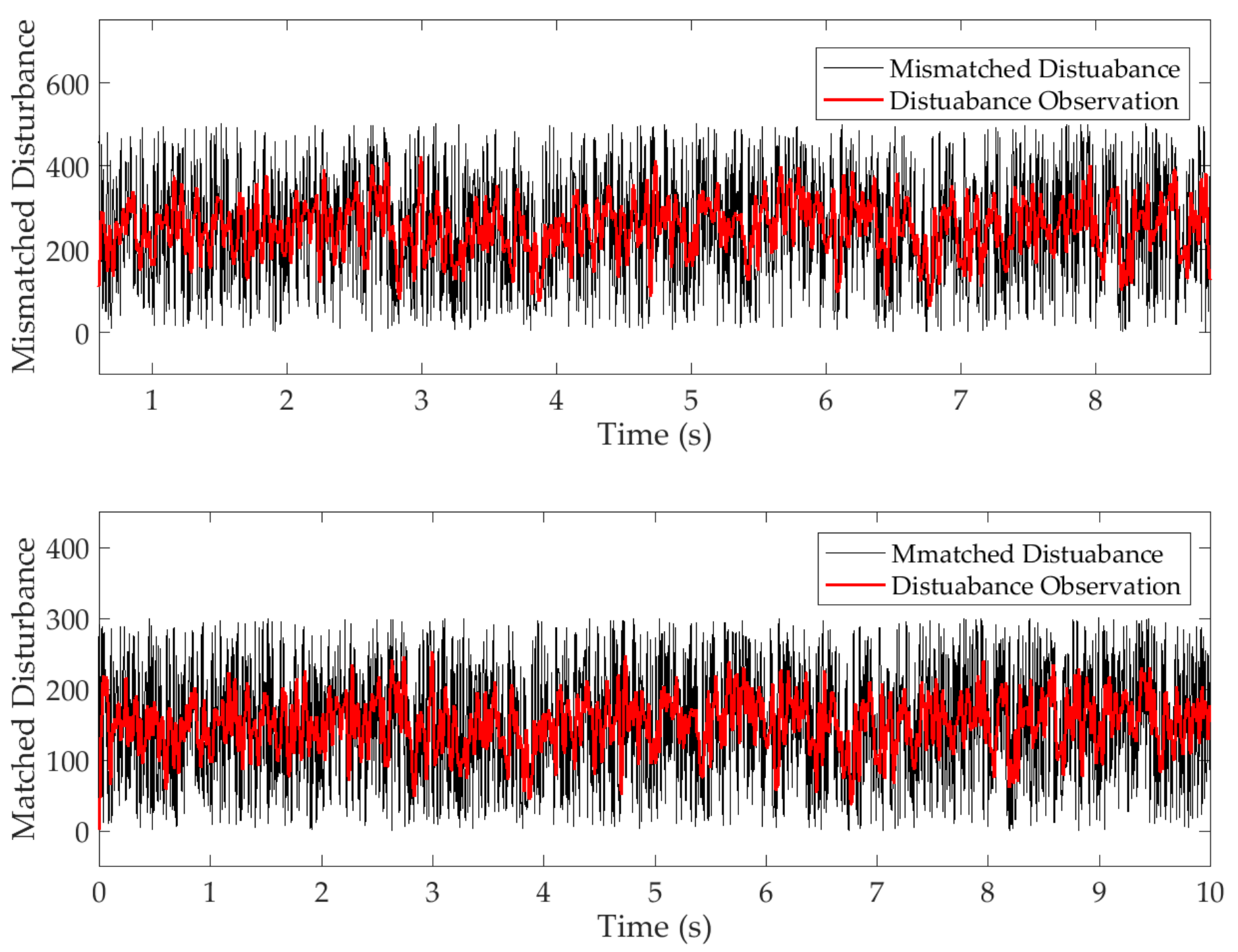
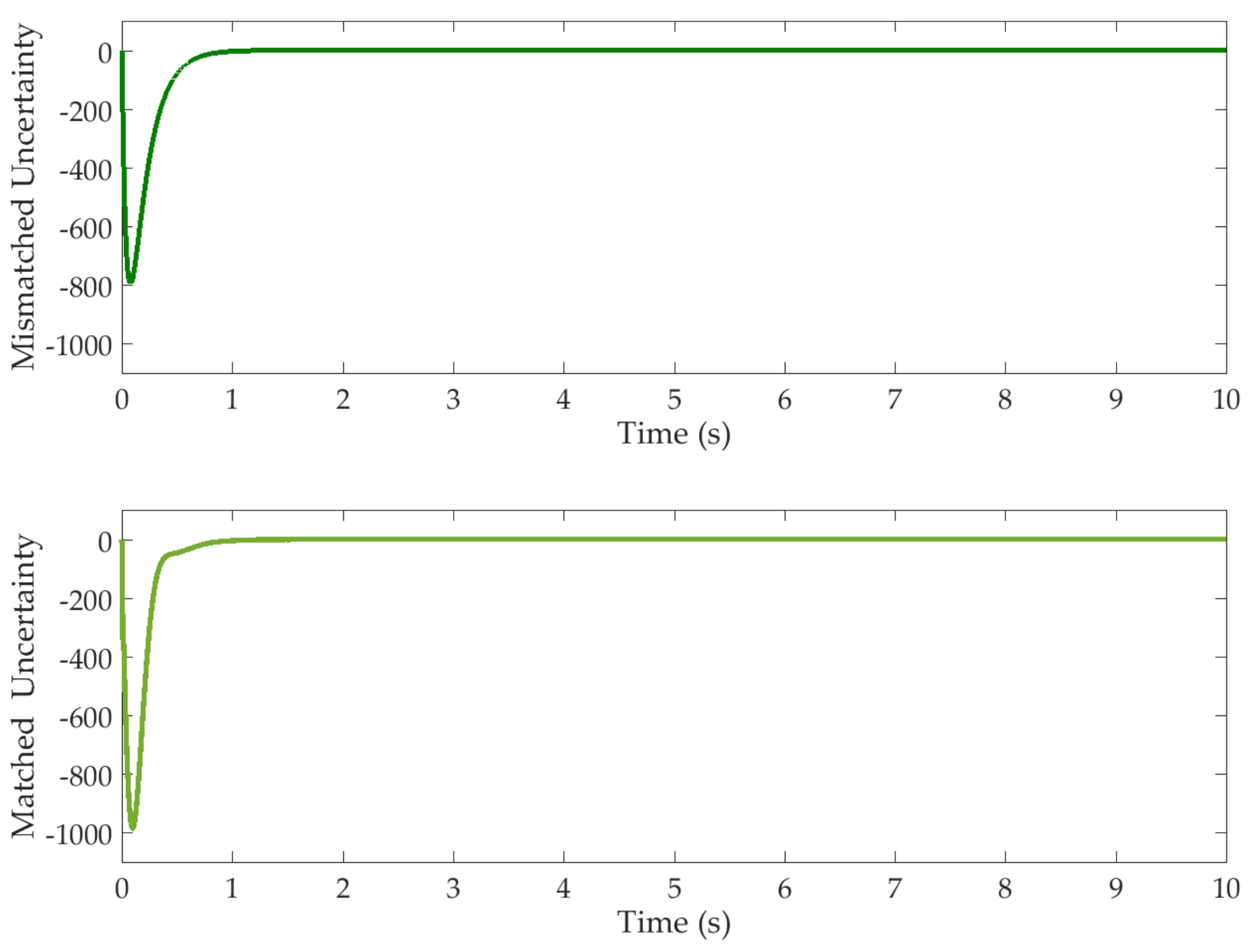
• Two extended state observers are constructed for each channel in a glue-dosing system that contains uncertainties. The matched and unmatched uncertainties are estimated, such that the compound controller can compensate for them in a feed-forward manner;
• A compound controller is proposed, in combination with the prescribed performance method and the sliding-mode dynamic surface control method. With this control scheme, the transient and steady-state performance of the system are guaranteed, by limiting the output error to a specified range. By introducing a specific error conversion function, the prescribed performance specifications are incorporated into a closed-loop design with the controller, which effectively promotes the derivation of the design process;
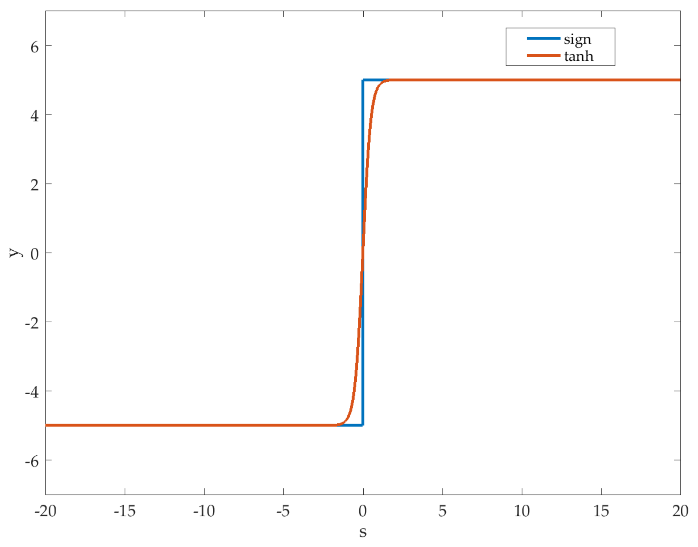
• Considering that the observers cannot completely estimate and compensate for the uncertainty in each channel, the sliding-mode surface with the hyperbolic tangent function is introduced into the dynamic surface, in which the complexity explosion problem is addressed by introducing a first-order filter into the control steps, and the learning burden of the ESOs is reduced without chattering to the actuator, in order to avoid high-gain or high-frequency feedback.

The remainder of this paper is organized as follows: In Section 2, the particleboard glue-dosing process is introduced and the mathematical model is established for the following design and analysis. Section 3 provides the design process of the compound controller design process, including the PPC scheme, the ESOs, and the SMDSC method. The convergence of the closed-loop system is proven after the design of the controller. In Section 4, simulation results are provided, in order to verify the effectiveness of the proposed controller. Finally, our conclusions are given in Section 5.

2. Process and Plant Description

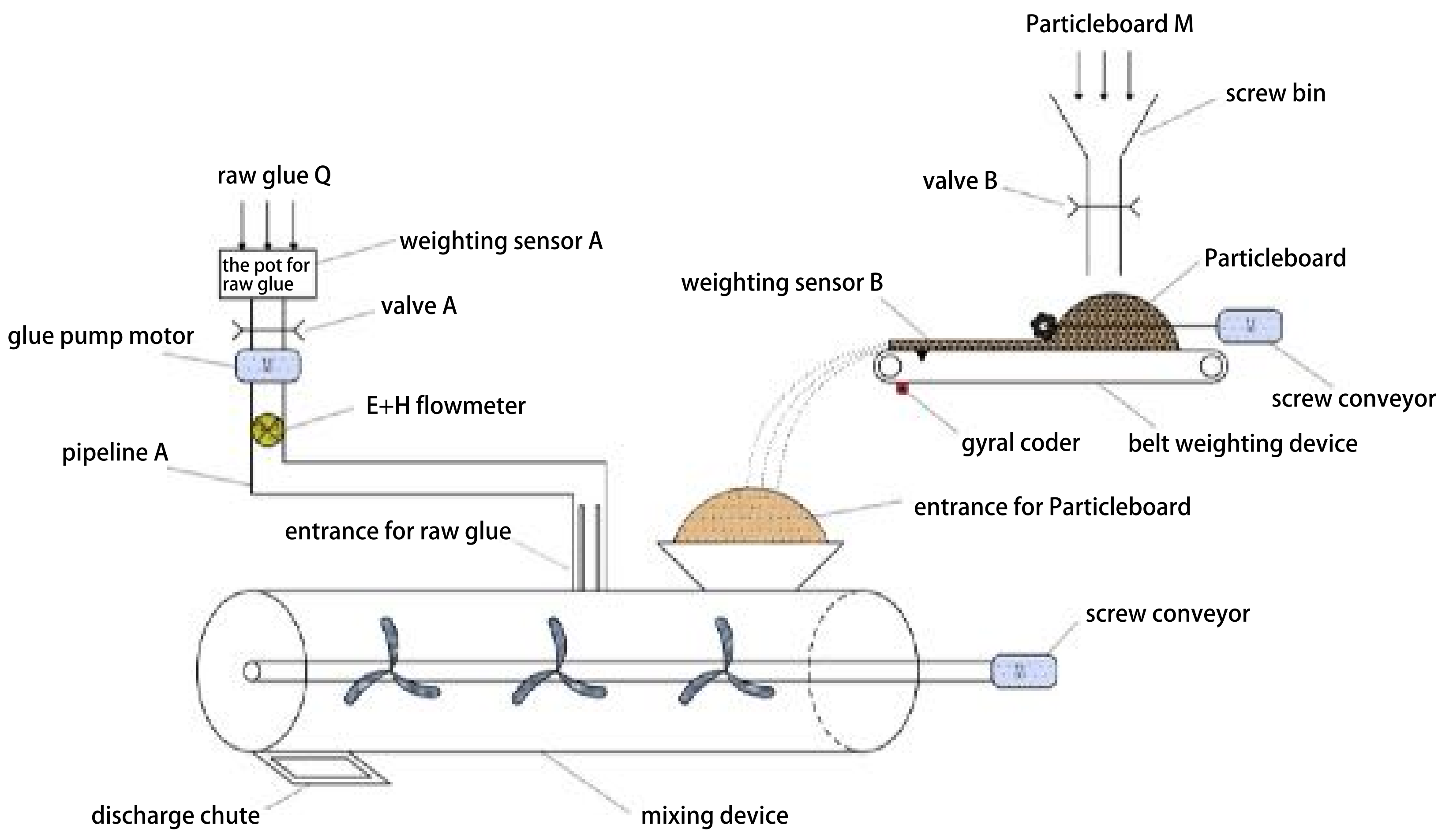
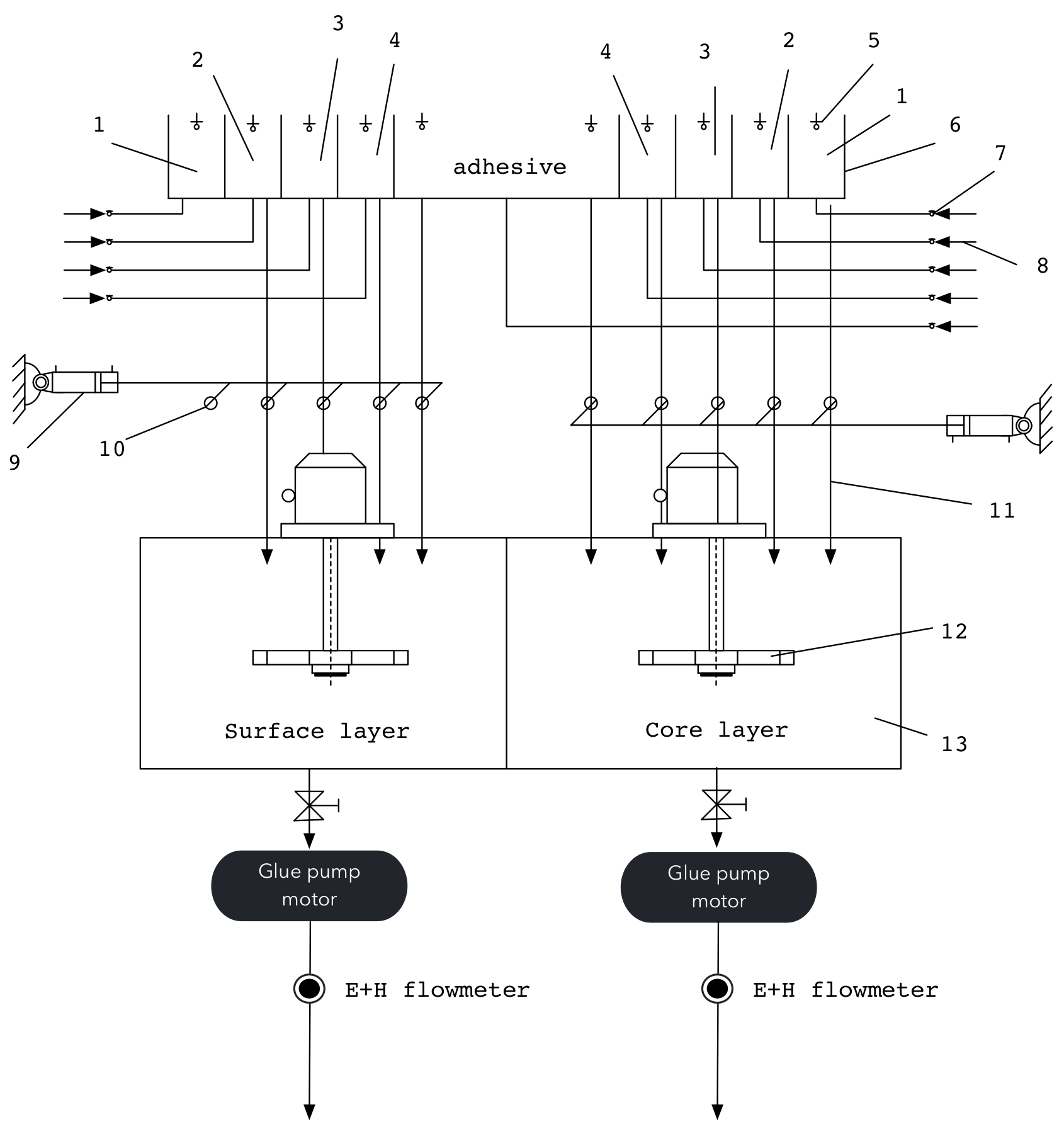
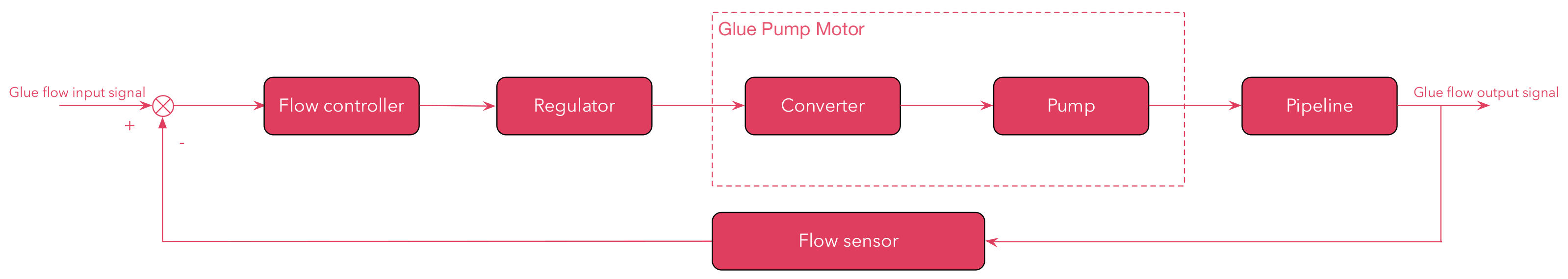
2.1. Particleboard Glue-Dosing Process

The glue-dosing process is one of the most important parts of particleboard production, as it defines its technical level. The key to judging the quality of the effects of the control of a glue-dosing system is determining whether the glue can be accurately mixed, according to the requirements of the formula. In the process of production, too much glue will lead to a high water content in the finished particleboard, which can result in blistering phenomena and increases in the rates of product waste, raw material wastes, and production costs. If the amount of glue is too small, the physical and mechanical properties of the particleboard, such as its static bending strength, plane tensile strength, and so on, may be reduced. The plasticity of the particleboard will also be reduced, which makes it more difficult to press, thus ultimately reducing the quality of the product. Therefore, the level of automation of particleboard glue-dosing control devices and actuators directly affects the market competitiveness and benefits of particleboard production enterprises.

Such a system is divided into two subprocesses—glue preparation and glue-dosing. The schematic diagrams of the particleboard glue-dosing process are shown in Figure 1 and Figure 2. In the preparation part, the volumes of various raw materials (including the curing agent, waterproofing agent, curing buffer agent, water, and adhesive) are measured using a liquid level detector. The raw materials then flow into the mixing case, as a result of gravity. A ball valve is used to control the amounts of raw materials. All raw materials are mixed by an agitator in the mixing case, which is divided into sections dedicated to the surface layer and the core layer of the particleboard.

After mixing the prepared glue in the glue mixing case, it flows to the glue pump motor through valve A and is measured by an E + H electromagnetic flowmeter. Then, the glue is transported to the mixing device through pipeline A. At the same time, the raw shaving particles are weighed by a belt-weighting device, then transported to the mixing device. In the process of the production of particleboard, two separate mixing devices are needed to stir the surface- and core-layer particles. For convenience, only one mixing device is shown in Figure 2. In order to simulate the process, a set of particleboard glue-dosing equipment (GMD-A-type) was used for this study, which is shown in Figure 3. The core actuator of the simulated system—that is, the glue pump motor—is shown in Figure 4.

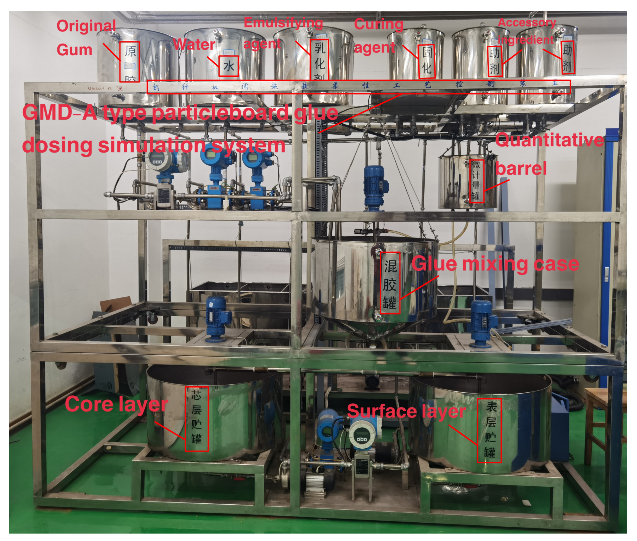
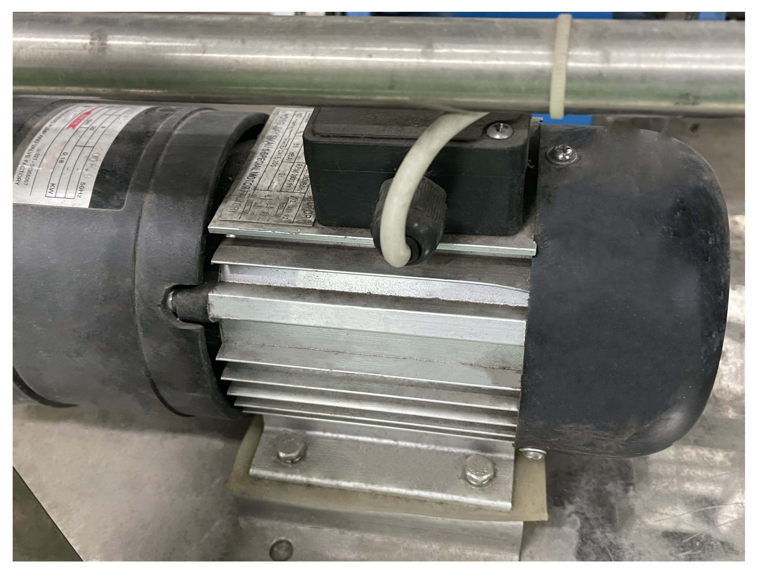
2.2. Plant Description

A schematic diagram of the glue-dosing process is shown in Figure 5. The desired glue flow signal is delivered to the system, and the real-time flow signal is measured by the electromagnetic flowmeter, which sends the output value back to the control system. By determining the difference between the two signals, the error value is obtained, which is processed by the flow regulator. Then, the regulation and the speed of the motor are changed by the frequency converter, in order to change the running speed of the gear pump. The change in the speed of the gear pump speed adjusts the amount of glue sent into the pipeline for glue flow control.

In [45], a simple and practical mathematical model for a variable-frequency voltage-regulating power supply system was derived. For a converter under the condition of a constant voltage frequency ratio in a squirrel cage motor, the linear model, with small deviation, is constructed as follows:

$$J\dot{\omega }=-(D+p{K}_0)\omega +p{K}_0{\omega }_1-pm,$$

(1)

$$K_0=\frac{p}{r_2}{\left(\frac{V_{10}}{{\omega }_{10}}\right)}^2,$$

(2)

where ${\omega }_1$ and $\omega$ represent the deviations of the stator’s power frequency and the rotor’s electric angular velocity, respectively; $V_{10}$ and ${\omega }_{10}$ represent the voltage and frequency values of the stator power supply at the static work point, respectively; p is the role pair number; $r_2$ represents the rotor resistance converted to the stator side; D represents the friction coefficient; m is the deviation of the load torque.

For the pump load, the torque is proportional to the square of the speed. When linearized with a small deviation, the relation of the deviation is [46]:

$$m=K_m\omega ,$$

(3)

where $K_m$ is a torque deviation constant. By substituting Equations (2) and (3) into Equation (1), the mathematical expression for the load of the pump motor is obtained as:

$$J\dot{\omega }=-(D+p{K}_0+K_m)\omega +p{K}_0{\omega }_1,$$

(4)

the transfer function is:

$$\frac{\omega \left(s\right)}{{\omega }_1\left(s\right)}=\frac{K_d}{1+T_{d}s},$$

(5)

where $T_d=(D+p{K}_0+K_m)/J$, $K_d=p{K}_0/J$.

In the working process of the motor, the flywheel torque of its driving system is usually greater than the rate at which the speed of the load fluctuates. This can be ensured by adjusting the appropriate times for acceleration and deceleration. For the pump load, in order to reduce the water hammer effect, an integrator must be set, causing the output frequency to change slowly when the control signal changes:

$$\frac{{\omega }_1\left(s\right)}{c\left(s\right)}=\frac{K_v}{1+T_{v}s},$$

(6)

where c represents the control signal processed by the regulator and $K_v$ and $T_v$ are controller parameters.

In order to eliminate the static error in the control system, the flow regulator is set as an integral loop:

$$\frac{c\left(s\right)}{u\left(s\right)}=\frac{1}{C_{u}s},$$

(7)

where $C_u$ is a regulator parameter.

As for the mathematical model of the pump–pipeline part of the system, a set of partial differential equations can be used to fit the response curve of the glue flow:

$$\frac{y\left(s\right)}{\omega \left(s\right)}=\frac{(K_b-K_g)s}{1+T_{b}s},$$

(8)

where y represents the glue flow, $K_b$ is the control constant, $K_g$ represents the differential coefficient of the liquid’s antiregulation role, and $T_b$ represents the time constant of the glue inertia.

Through the above analysis, the nominal mathematical model of the dosing system for the glue pump motor is obtained through the combination of Equations (5)–(8):

$$\frac{y\left(s\right)}{u\left(s\right)}=\frac{(K_b-K_g)K_v{K}_d}{C_u(1+T_{b}s)(1+T_{d}s)(1+T_{v}s)}.$$

(9)

As the actuator and sensor can be disturbed in the working process of the glue pump motor system, they will enter the nonlinear region under high-frequency conditions. In the pump–pipeline part of the system, the pipeline pressure has an impact on the glue flow. Therefore, the state equation of the system with disturbances and uncertainties is obtained by referring to the nominal model given in Equation (10):

$$\left\{\begin{array}{c}\dot{x_1}=x_2\hfill \\ \dot{x_2}=x_3+\Delta g(x_1,x_2,x_3)+d_1\hfill \\ \dot{x_3}=f(x_1,x_2,x_3)+ku+\Delta f(x_1,x_2,x_3)+d_2\hfill \\ y=x_1\hfill \end{array},\right.$$

(10)

where $\Delta g(x_1,x_2,x_3)=\Delta g_1{x}_1+\Delta g_2{x}_2+\Delta g_3{x}_3$ and $\Delta f(x_1,x_2,x_3)=\Delta f_1{x}_1+\Delta f_2{x}_2+\Delta f_3{x}_3$ represent the unmodeled dynamics, $d_1$ and $d_2$ are the external disturbances to the system, $k=(K_b-K_g)K_v{K}_d$, $f(x_1,x_2,x_3)=f_1{x}_1+f_2{x}_2+f_3{x}_3,f_1=C_u,f_2=(T_b{T}_d+T_b{T}_v+T_d{T}_v)C_u$, and $f_3=T_b{T}_d{T}_v{C}_u$.

Assumption 1.

The external disturbance $d_i$ and the unmodeled dynamics are bounded by $\left|d_i\right|⩽D_i(i=1,2)$ and $\left|\Delta g(x_1,x_2,x_3)\right|\le G$,$\left|\Delta f(x_1,x_2,x_3)\right|\le F$, in which $D_i$, G, and F are all unknown positive constants.

Assumption 2.

The desired trajectory y is a known bounded function of time, for which there exists a known bounded derivative.

Assumption 3.

The state $x=[x_1,x_2,x_3]$ is available for measurement.

Remark 1.

The disturbances $d_i(i=1,2)$ are caused by the operations of the motor and sensor, which are unknown and bounded. $\Delta g$ and $\Delta f$ represent the uncertainty of the parameters and some unmodeled dynamics caused by the application of the glue, as well as the pressure and temperature. Assumption 3 is given for the subsequent observer and controller design.

3. Controller Design

3.1. Prescribed Performance Control

In the design of the prescribed performance control, the performance function and error transfer function are proposed to control the steady-state and transient performance of the system, including the overshoot and convergence rate.

Considering the controlled system shown in Equation (10), we define the tracking error as follows:

$$e=y-y_d,$$

(11)

where $y_d$ is the desired tracking signal. In order to ensure the transient performance of the system, the performance function is defined as follows:

Definition 1.

A smooth function $\rho :{\Re }_{+}\to {\Re }_{+}$ is called a performance function ($\rho \in \mathcal{P}$) if [15]:

• ρ is positive and decreasing;
• ${\lim }_{t\to \infty }\rho \left(t\right)={\rho }_{\infty }>0$.

In general, a function that satisfies the conditions in Definition 1 can be used as a performance function. For this paper, the following performance function was selected [31]:

$$\rho \left(t\right)=(\rho \left(0\right)-\rho (\infty ))e^{-\nu t}+\rho (\infty ),$$

(12)

where $\rho \left(0\right)$ is the initial value of the performance function, $\rho (\infty )$ is a positive constant, and $\nu$ is an adjustable parameter.

To ensure the transient performance of the system, the tracking error of the system output satisfies the following inequality:

$$\left\{\begin{array}{c}-\delta \rho \left(t\right)<e<\rho \left(t\right),e\left(0\right)>0\hfill \\ -\rho \left(t\right)<e<\delta \rho \left(t\right),e\left(0\right)<0\hfill \end{array},\right.$$

(13)

where $0\le \delta \le 1$.

According to Equation (13), the tracking error is constrained in a specified range and, finally, converges to an arbitrarily small area, in which the upper bound of the system stability error is determined by $\rho (\infty )$. The slope of the performance function, $\rho \left(t\right)$, is the lower convergence speed of the tracking error, and the overshoot is constrained by $\delta \rho \left(0\right)$.

Through the above analysis, it can be found that the transient performance of the system can be controlled by changing the performance function shown in Equation (12). However, the form of the constraint is an inequality, which may lead to difficulties in the subsequent controller design. Under this condition, the error transfer function is introduced, in order to solve this problem.

Substituting Equation (11) into Equation (13) gives:

$$\left\{\begin{array}{c}-\delta \rho \left(t\right)+y_d<y<\rho \left(t\right)+y_d,e\left(0\right)>0\hfill \\ -\rho \left(t\right)+y_d<y<\delta \rho \left(t\right)+y_d,e\left(0\right)<0\hfill \end{array}.\right.$$

(14)

According to Equation (14), the nature of the prescribed system performance control problem is a kind of output-constrained problem, which the BLF method can effectively solve. The following BLF candidate was chosen:

$$V_1=\frac{1}{2}log\frac{1}{1-{\epsilon }^2},$$

(15)

where $\epsilon$ is the error transformation function, and

$$\epsilon =\frac{2z_1-(p\left(t\right)+q\left(t\right))}{q\left(t\right)-p\left(t\right)},$$

(16)

where $z_1=e$, $p\left(t\right)=-\rho \left(t\right)$, and $q\left(t\right)=\delta \rho \left(t\right)$.

For the convenience of analysis in the subsequent design, the following lemmas are introduced:

Lemma 1 ([47]).

Let $\mathcal{Z}=\{\xi \in \mathbb{R}:\left|\xi \right|<1\}\subset \mathbb{R}$ and $\mathcal{N}={\mathbb{R}}^l\times \mathcal{Z}\in {\mathbb{R}}^{l+1}$ be open sets. Considering the system:

$$\dot{\eta }=h(t,\eta ),$$

where $\eta ={[\mathcal{W},\xi ]}^T$, the function $h:{\mathbb{R}}_{+}\times \mathcal{N}\to {\mathbb{R}}^{l+1}$ is piecewise continuous at time t for ${\mathbb{R}}_{+}$ and satisfies the local Lipschitz condition for η. Assuming the existence of a connected and differentiable positive-definite function $\mathcal{U}:{\mathbb{R}}^l\times {\mathbb{R}}_{+}\to {\mathbb{R}}_{+}$, ${\mathcal{V}}_1:\mathcal{Z}\to {\mathbb{R}}_{+}$ satisfies

$$\left|\xi \right|\to 1,{\mathcal{V}}_1\left(\xi \right)\to \infty ,{\gamma }_1\left(∥\mathcal{W}∥\right)⩽\mathcal{U}(\mathcal{W},t)\le {\gamma }_1\left(∥\mathcal{W}∥\right),$$

where ${\gamma }_1$ and ${\gamma }_2$ are class $K_{\infty }$ functions. Let $\mathcal{V}\left(\eta \right)={\mathcal{V}}_1\left(\xi \right)+\mathcal{U}(\mathcal{W},t)$ and $\xi \left(0\right)\in \mathcal{Z}$. If the following inequality holds:

$$\dot{\mathcal{V}}=\frac{\partial \mathcal{V}}{\partial \eta }\le 0,$$

then $\xi \left(t\right)\in \mathcal{Z}$ when $t\ge 0$.

Lemma 2 ([48]).

For $\left|\epsilon \right|<1$ and any positive integer a, the following inequality holds:

$$log\frac{1}{1-{\epsilon }^{2a}}<\frac{{\epsilon }^{2a}}{1-{\epsilon }^{2a}}.$$

3.2. Extend State Observer Design

As the traditional ESO [42] can only observe and compensate for the matching uncertainty, it is not suitable for the system model given in Equation (10). By referring to [44], two ESOs were constructed:

$$\left\{\begin{array}{c}{\dot{\widehat{x}}}_1={\widehat{x}}_2+{\eta }_1{\omega }_{e1}(x_1-{\widehat{x}}_1)\hfill \\ {\dot{\widehat{x}}}_2=x_3+{\widehat{x}}_{e1}+{\eta }_2{\omega }_{e1}^2(x_1-{\widehat{x}}_1)\hfill \\ {\dot{\widehat{x}}}_{e1}={\eta }_3{\omega }_{e1}^3(x_1-{\widehat{x}}_1)\hfill \end{array},\right.$$

(17)

$$\left\{\begin{array}{c}{\dot{\widehat{x}}}_3=f(x_1,x_2,x_3)+ku+{\widehat{x}}_{e2}+{\zeta }_1{\omega }_{e2}(x_3-{\widehat{x}}_3)\hfill \\ {\dot{\widehat{x}}}_{e2}={\zeta }_2{\omega }_{e2}^2(x_3-{\widehat{x}}_3)\hfill \end{array},\right.$$

(18)

where $\widehat{x_i}(i=1,2,3)$ represent the observations of the state $x_i(i=1,2,3)$, the unmatched uncertainties $\Delta g(x_1,x_2,x_3)+d_1$ are extended as the additional state $x_{e1}$, the matched uncertainties $\Delta f(x_1,x_2,x_3)+d_2$ are extended as the additional state $x_{e2}$, ${\widehat{x}}_i(i=1,2)$ are the estimated values, and ${\omega }_{ei}$, ${\zeta }_i(i=1,2)$, and ${\eta }_i(i=1,2,3)$ are the tuning parameters for the observer bandwidth.

The system model shown in Equation (10) can be rewritten as follows:

$$\left\{\begin{array}{c}{\dot{x}}_1=x_2\hfill \\ {\dot{x}}_2=x_3+x_{e1}\hfill \\ {\dot{x}}_{e1}=h_1\left(t\right)\hfill \end{array},\right.$$

(19)

$$\left\{\begin{array}{c}{\dot{x}}_3=f(x_1,x_2,x_3)+ku+x_{e2}\hfill \\ {\dot{x}}_{e2}=h_2\left(t\right)\hfill \end{array},\right.$$

(20)

where $h_1\left(t\right)$, $h_2\left(t\right)$ represent the rate of change of the uncertainty, which are unknown but bounded by $H_1$ and $H_2$, which are expressed in terms of $D_i$, $F_i$, $G_i$, $\left|x_i\right|$, and u. The observational errors are defined as $\widetilde{x_i}=x_i-{\widehat{x}}_i$ and ${\tilde{x}}_{ei}=x_{ei}-{\widehat{x}}_{ei}$. Theorem 1 is given as follows.

Theorem 1.

Consider the system model described in (19). By appropriately choosing the observer gain $[{\eta }_1,{\eta }_2,{\eta }_3]$ providing the Hurwitz matrix (A3), there exist the positive-definite matrices P and Q that satisfy the Lyapunov Equation (A6). The estimated error ε is bounded by a region Ω described in (A9). As for Equation (12), the observer gain $[{\zeta }_1,{\zeta }_2]$ is chosen to provide the Hurwitz matrix (A12); there exist the positive-definite matrices $P_1$ and $Q_1$ that satisfy the Lyapunov Equation (A15). The estimated error ϖ is bounded by a region ${\mathsf{\Omega }}_1$ described in (A18).

Proof of Theorem 1.

See Appendix A. □

Remark 2.

Based on Theorem 1, the tuning parameter ${\tilde{x}}_{e1}$ is adjustable for reducing the boundary Ω and the tuning parameter ${\tilde{x}}_{e2}$ is adjustable for reducing the boundary ${\mathsf{\Omega }}_1$.

3.3. Design Steps for a Compound Controller

By using the sliding-mode dynamic surface control method combined with the design of the prescribed performance control described in Section 3.1 and the ESOs described in Section 3.2, the compound controller was designed. First, an appropriate BLF candidate was selected to construct the error conversion function, in order to solve the problem of the limitations of the system output, thus ensuring the preset performance of the system. Second, the error transfer function was introduced in the first subsystem of the process of dynamic surface design, while a first-order filter was applied in the second subsystem. The derivative of the virtual control input was calculated with the DSC method, in order to avoid the expansion of the differential term caused by the backstepping control method. Finally, the new variable was used as the input to the third subsystem, and the observations of the unknown uncertainties of the ESOs were used to realize the design of the control input.

Step 1: The tracking error of the first subsystem is:

$$z_1=x_1-y_d,$$

(21)

and the derivative with respect to time for $z_1$ is:

$$\begin{array}{cc}{\dot{z}}_1\hfill & ={\dot{x}}_1-{\dot{y}}_d\hfill \\ \hfill & =x_2-{\dot{y}}_d.\hfill \end{array}$$

(22)

The Lyapunov function is chosen as shown in Equation (15) for the first subsystem, and the derivative is:

$${\dot{V}}_1=\dot{\epsilon }\frac{\epsilon }{1-{\epsilon }^2}.$$

(23)

The derivative of the error transformation shown in Equation (16) with respect to time is as:

$$\dot{\epsilon }=\frac{2{\dot{z}}_1-(\dot{p}+\dot{q})}{q-p}-\frac{[2z_1-(p+q)](\dot{q}-\dot{p})}{{(q-p)}^2}.$$

(24)

Define the second subsystem tracking error $z_2$:

$$z_2=x_2-{\alpha }_1,$$

(25)

where ${\alpha }_1$ is the virtual control variable.

Considering Equations (22)–(25), we have:

$${\dot{V}}_1=[\frac{2(z_2+{\alpha }_1-{\dot{y}}_d)}{q-p}-2\frac{z_1(\dot{q}-\dot{p})-p\dot{q}+\dot{p}q}{{(q-p)}^2}]\frac{\epsilon }{1-{\epsilon }^2}.$$

(26)

To facilitate subsequent stability analyses in Section 3.4, the virtual control for the second subsystem ${\alpha }_1$ is designed as:

$${\alpha }_1=-k_1{z}_1+\frac{k_1(p+q)}{2}+{\dot{y}}_d+\frac{z_1(\dot{q}-\dot{p})-p\dot{q}+\dot{p}q}{{(q-p)}^2},$$

(27)

where $k_1>0$ is the tuning parameter.

Substituting Equation (27) to (26), we have:

$${\dot{V}}_1=\epsilon (-\frac{k_1\epsilon }{1-{\epsilon }^2}+\frac{2z_2}{(1-{\epsilon }^2)(q-p)}),$$

(28)

where $\left|\epsilon \right|<1$ according to Lemma 1.

Step 2: By differentiating the second subsystem tracking error $z_2$, we have:

$$\begin{array}{cc}{\dot{z}}_2\hfill & ={\dot{x}}_2-{\dot{\alpha }}_1\hfill \\ \hfill & =x_3+x_{e1}-{\dot{\alpha }}_1.\hfill \end{array}$$

(29)

According to Equation (26), the derivative of the virtual control ${\alpha }_1$ with respect to time is as:

$$\begin{array}{cc}{\dot{\alpha }}_1=\hfill & -k_1{\dot{z}}_1+\frac{k_1(\dot{p}+\dot{q})}{2}+{\ddot{y}}_d+\frac{[{\dot{z}}_1(\dot{q}-\dot{p})+z_1(\ddot{q}-\ddot{p})-p\ddot{q}+\ddot{p}q]}{q-p}\hfill \\ \hfill & -\frac{[z_1(\dot{q}-\dot{p})-p\dot{q}+\dot{p}q](\dot{q}-\dot{p})}{{(q-p)}^2}.\hfill \end{array}$$

(30)

The Lyapunov function of the second subsystem is chosen as:

$$V_2=\frac{1}{2}{z}_2^2.$$

(31)

For the reason of mismatch uncertainty, the virtual control of the third subsystem ${\alpha }_2$ combined with the ESO is designed as:

$${\alpha }_2=-k_2{z}_2+{\dot{\alpha }}_1-\frac{2\epsilon }{(1-{\epsilon }^2)(q-p)}-{\widehat{x}}_{e1},$$

(32)

where $k_2>0$ is the tuning parameter, which denotes the feedback gain.

The input ${\alpha }_2$ is passed through a first-order low-pass filter, and we take its output, ${\alpha }_{2d}$, as a new virtual control variable in the third subsystem:

$$\tau {\dot{\alpha }}_{2d}+{\alpha }_{2d}={\alpha }_2,$$

(33)

where $\tau$ is a time constant and ${\alpha }_{2d}\left(0\right)={\alpha }_2\left(0\right)$.

Hence, the tracking error of the third subsystem $z_3$ is:

$$\begin{array}{cc}{z}_3=\hfill & x_3-{\alpha }_{2d}\hfill \\ \hfill =& {\dot{z}}_2+{\dot{\alpha }}_1-x_{e1}-{\alpha }_{2d}.\hfill \end{array}$$

(34)

The filter error is:

$$e_{\alpha }={\alpha }_{2d}-{\alpha }_2.$$

(35)

By differentiating Equation (31):

$$\begin{array}{cc}{\dot{V}}_2=\hfill & z_2{\dot{z}}_2\hfill \\ \hfill =& z_2(z_3+x_{e1}+{\alpha }_{2d}-{\dot{\alpha }}_1)\hfill \\ \hfill =& z_2>(z_3+x_{e1}+e_{\alpha }-k_2{z}_2+{\dot{\alpha }}_1-\frac{2\epsilon }{(1-{\epsilon }^2)(q-p)}-{\widehat{x}}_{e1}-{\dot{\alpha }}_1>)\hfill \\ \hfill =& -k_2{z}_2^2+z_2{z}_3+e_{\alpha }{z}_2-\frac{2\epsilon z_2}{(1-{\epsilon }^2)(q-p)}+z_2{\tilde{x}}_{e1}.\hfill \end{array}$$

(36)

Step 3: By differentiating the third subsystem tracking error $z_3$, we have:

$$\begin{array}{cc}{\dot{z}}_3=\hfill & {\dot{x}}_3-{\dot{\alpha }}_{2d}\hfill \\ \hfill =& f\left(x\right)+ku+x_{e2}-{\dot{\alpha }}_{2d},\hfill \end{array}$$

(37)

where:

$$\begin{array}{cc}\hfill {\dot{\alpha }}_{2d}=& {\dot{\alpha }}_{2dc}+{\dot{\alpha }}_{2du}\hfill \\ \hfill {\dot{\alpha }}_{2dc}=& \frac{\partial {\alpha }_{2d}}{\partial t}+\frac{\partial {\alpha }_{2d}}{\partial x_1}{x}_2+\frac{\partial {\alpha }_{2d}}{\partial x_2}(x_3+{\widehat{x}}_{e1})+\frac{\partial {\alpha }_{2d}}{\partial {\widehat{x}}_{e1}}{\dot{\widehat{x}}}_{e1}\hfill \\ \hfill {\dot{\alpha }}_{2du}=& \frac{\partial {\alpha }_{2d}}{\partial x_2}{\widehat{x}}_{e1},\hfill \end{array}$$

(38)

In Equation (38), ${\dot{\alpha }}_{2dc}$ indicates that known and computable, which is used in the controller design, and ${\dot{\alpha }}_{2du}$ indicates the unknown part must be suppressed by some robust feedback due to uncertain nonlinearity [44]. ${\dot{\alpha }}_{2d}$ can be obtained from Equation (32). Considering that the observation cannot completely compensate for this uncertainty, it is necessary to strengthen the robust control in the third subsystem.

The third subsystem is defined as the sliding-mode surface referring to [49]:

$$s=z_3.$$

(39)

The Lyapunov function of the third subsystem is defined as:

$$V_3=\frac{1}{2}{s}^2,$$

(40)

and the derivative with respect to time is:

$$\begin{array}{cc}\hfill {\dot{V}}_3=& s\dot{s}\hfill \\ \hfill =& s(f\left(x\right)+ku+x_{e2}-{\dot{\alpha }}_{2d}).\hfill \end{array}$$

(41)

Based on Equations (37) and (41) and the SMC method, the control law u is designed as:

$$u=\frac{1}{k}(-k_3{z}_3-f\left(x\right)-z_2-{\widehat{x}}_{e2}+{\dot{\alpha }}_2-\gamma sgn\left(z_3\right)),$$

(42)

where $k_3$ is the tuning parameter and $\gamma$ is the switching term gain, which satisfies $\gamma \ge D_2+F$.

Remark 3.

In order to prevent the observers from being affected by noise interference, the appropriate observer gains were not chosen too high. Although this will lead to the decline of observation performance, the prescribed performance and sliding-mode dynamic surface control were used as a supplement to further improve the steady-state performance of the system. As for the control gain γ in sliding-mode control, let $\gamma \ge D_2+F$ to eliminate disturbance and uncertainty.

Considering the chattering of the control signal induced by the switching term $-\gamma sgn\left(z3\right)$, which may lead to the actuators’ damage, a hyperbolic tanh function $\theta \left(s\right)$ was introduced instead of $sgn\left(s\right)$:

$$\theta \left(s\right)=\frac{e^{\frac{s}{\mu }}-e^{-\frac{s}{\mu }}}{e^{\frac{s}{\mu }}+e^{-\frac{s}{\mu }}}$$

(43)

where $\mu >0$. The comparison between $y=5\theta \left(s\right)$ and $y=5sgn\left(s\right)$ is shown in Figure 6. It can be seen that the hyperbolic tangent function $\theta \left(s\right)$ can realize a smooth transition and avoid system chattering caused by high-frequency switching.

The configuration of the compound controller obtained through the above analysis is shown in Figure 7.

3.4. Stability Analyses

In this section, the stability of the system is analyzed by constructing the Lyapunov function. Before that, the following preparations are given below. First, define a set of scalars as:

$$\begin{array}{cc}\hfill {\mathsf{\Omega }}_1:=& \left\{(y_d,{\dot{y}}_d,{\ddot{y}}_d):y_d^2+{\dot{y}}_d^2+{\ddot{y}}_d{)}^2\le \upsilon \right\},\hfill \\ \hfill {\mathsf{\Omega }}_2:=& \left\{log\frac{1}{1-{\epsilon }^2}+z_2+z_3+e_{\alpha }\le 2\varphi \right\},\hfill \\ \hfill {\kappa }_1=& w_2{\omega }_{e1}^2,{\kappa }_2=w_3{\omega }_{e1}^2\left|\frac{\partial {\alpha }_2}{\partial x_2}\right|,{\kappa }_3=w_3{\omega }_{e2},\hfill \\ \hfill {\varsigma }_1=& \frac{{\mu }_2}{2}(w_{e1}-1),{\varsigma }_2=\frac{{\mu }_3}{2}(w_{e2}-1),\hfill \\ \hfill \vartheta =& \frac{{\mu }_2}{2}{(\frac{∥P_1{\theta }_1∥{\left|h_1\left(t\right)\right|}_{max}}{{\omega }_{e1}^2})}^2+\frac{{\mu }_3}{2}{(\frac{∥P_2{\theta }_4∥{\left|h_2\left(t\right)\right|}_{max}}{{\omega }_{e2}^2})}^2\hfill \end{array}$$

(44)

where $\upsilon$, $\varphi$, $w_2$, $w_3$, ${\mu }_2$, ${\mu }_3$ are positive constants and $P_1$, $P_2$ are positive definite matrices satisfying ${\eta }^T{P}_1+P_1\eta =-I$, ${\zeta }^T{P}_2+P_2\zeta =-I$.

Differentiating Equation (34), we obtain that:

$$\begin{array}{cc}\hfill {\dot{e}}_{\alpha }=& {\dot{\alpha }}_{2d}-{\dot{\alpha }}_2\hfill \\ \hfill =& \frac{{\alpha }_2-{\alpha }_{2d}}{\tau }-(-k_2{\dot{z}}_2+{\ddot{\alpha }}_1-{\dot{z}}_1-{\dot{\widehat{x}}}_{e1})+\frac{\partial }{\partial t}\left(\frac{2\epsilon }{(1-{\epsilon }^2)(q-p)}\right)\hfill \\ \hfill =& -\frac{e_{\alpha }}{\tau }+L\hfill \end{array},$$

(45)

where $L=-(-k_2{\dot{z}}_2+{\ddot{\alpha }}_1-{\dot{z}}_1-{\dot{\widehat{x}}}_{e1})+\frac{\partial }{\partial t}\left(\frac{2\epsilon }{(1-{\epsilon }^2)(q-p)}\right)$.

The Lyapunov function is constructed as:

$$\begin{array}{cc}\hfill V=& \sum _{i=1}^3{V}_i+\frac{1}{2}(e_{\alpha }^2+{\mu }_2{\tilde{X}}_{12}^T{P}_1{\tilde{X}}_{12}+{\mu }_3{\tilde{X}}_3^T{P}_2{\tilde{X}}_3)\hfill \\ \hfill =& V_c+V_o\hfill \end{array},$$

(46)

where $V_c={\sum }_{i=1}^3{V}_i+\frac{1}{2}{e}_{\alpha }^2$, $V_o=\frac{1}{2}({\mu }_2{\tilde{X}}_{12}^T{P}_1{\tilde{X}}_{12}+{\mu }_3{\tilde{X}}_3^T{P}_2{\tilde{X}}_3)$.

Invoking Equations (28), (36), (41), and (44), the derivative of Equation (45) is:

$$\begin{array}{cc}\hfill {\dot{V}}_c=& \sum _{i=1}^3{\dot{V}}_i+e_{\alpha }{\dot{e}}_{\alpha }\hfill \\ \hfill =& -\frac{k_1{\epsilon }^2}{1-{\epsilon }^2}-k_2{z}_2^2-k_3{z}_3^2-\gamma \left|z_3\right|-\frac{e_{\alpha }^2}{\tau }+L{e}_{\alpha }+z_2{e}_{\alpha }+z_2{\tilde{x}}_{e1}+z_3{\tilde{x}}_{e2}\hfill \\ \hfill {\dot{V}}_o=& -\frac{1}{2}({\mu }_2{\omega }_{e1}{∥{\tilde{X}}_{12}∥}^2+{\mu }_3{\omega }_{e2}{∥{\tilde{X}}_3∥}^2)\hfill \\ \hfill & +{\mu }_2{\tilde{X}}_{12}^T{P}_1{\theta }_2\frac{h_1\left(t\right)}{{\omega }_{e1}^2}+{\mu }_3{\tilde{X}}_3^T{P}_2{\theta }_4\frac{h_2\left(t\right)}{{\omega }_{e2}}\hfill \end{array},$$

(47)

The upper bound M of L in Equation (46) is defined on set ${\mathsf{\Omega }}_1\times {\mathsf{\Omega }}_2$, then $\frac{L^2}{M^2}-1\le 0$. According to Lemma 2 and Young’s inequality:

$$\begin{array}{cc}\hfill {\dot{V}}_c\le & -k_{1}log\frac{1}{1-{\epsilon }^2}-k_2{z}_2^2-k_3{z}_3^2-\gamma \left|z_3\right|\hfill \\ \hfill & -\frac{e_{\alpha }^2}{\tau }+L{e}_{\alpha }+\left|z_2\right|\left|e_{\alpha }\right|+\left|z_2\right|\left|{\tilde{x}}_{e1}\right|+\left|z_3\right|\left|{\tilde{x}}_{e2}\right|\hfill \\ \hfill \le & -k_{1}log\frac{1}{1-{\epsilon }^2}-k_2{z}_2^2-k_3{z}_3^2-\gamma \left|z_3\right|\hfill \\ \hfill & -\frac{e_{\alpha }^2}{\tau }+\frac{L^2{e}_{\alpha }^2+1}{2}+\frac{z_2^2+e_{\alpha }^2}{2}+\frac{z_2^2+{\tilde{x}}_{e1}^2}{2}+\frac{z_3^2+{\tilde{x}}_{e2}^2}{2}\hfill \\ \hfill \le & -k_{1}log\frac{1}{1-{\epsilon }^2}-\gamma \left|z_3\right|-(k_2-1)z_2^2-(k_3-\frac{1}{2})z_3^2\hfill \\ \hfill & -(\frac{1}{\tau }-\frac{1+L^2}{2})e_{\alpha }^2+\frac{1}{2}\Delta \hfill \end{array},$$

(48)

where $\Delta ={\tilde{x}}_{e1}^2+{\tilde{x}}_{e2}^2$, which depends on the observation error from the observation. Based on Remark 2, let ${\Delta }_{max}\ge \Delta$.

Consequently, the tuning parameters are chosen as:

$$k_1\ge \varrho ,k_2-1\ge \varrho ,k_3-\frac{1}{2}\ge \varrho ,\frac{1}{\tau }\ge \frac{(1+M^2)}{2}+\varrho ,$$

(49)

where $\varrho$ is a very small positive constant, and then:

$${\dot{V}}_c\le -2\varrho V_c+\frac{1}{2}{\Delta }_{max},$$

(50)

Lemma 3.

For $V:[0,\infty )\in R$, the solution of inequality $\dot{V}\le -\alpha V+f$, $\forall t\ge t_0\ge 0$ is:

$$V\left(t\right)\le e^{-\alpha (t-t_0)}V{\left(t\right)}_0+{\int }_{t_0}^t{e}^{-\alpha (t-\tau )}f\left(\tau \right)d\tau ,$$

(51)

where α is an arbitrary constant.

Proof of Lemma 3.

See Appendix B. □

According to Lemma 3, the solution of Equation (49) is:

$$\begin{array}{cc}\hfill V_c\le & e^{-\varrho (t-t_0)}{V}_c\left(t_0\right)+\frac{1}{2}{\Delta }_{max}^2{\int }_{t_0}^t{e}^{-\varrho (t-\tau )}d\tau \hfill \\ \hfill =& e^{-\varrho (t-t_0)}{V}_c\left(t_0\right)-\frac{1}{2\varrho }{\Delta }_{max}^2(1-e^{-\varrho (t-\tau )})\hfill \end{array},$$

(52)

where the Lyapunov function $V_c\left(t\right)=\frac{1}{2\varrho }{\Delta }_{max}^2,t\to \infty$, and the derivative ${\dot{V}}_c$ can be ensured to converge to zero exponentially.

We define a positive definite matrix, $\mathsf{\Lambda }$, as:

$$\mathsf{\Lambda }=\left[\begin{array}{ccc}{\mathsf{\Lambda }}_1& 0& {\mathsf{\Lambda }}_3\\ 0& {\varsigma }_1& 0\\ {\mathsf{\Lambda }}_3^T& 0& {\mathsf{\Lambda }}_2\end{array}\right],$$

(53)

where ${\mathsf{\Lambda }}_1=\left[\begin{array}{cc}{\omega }_2& -\frac{{\omega }_2}{2}\\ -\frac{{\omega }_2}{2}& {\omega }_3\end{array}\right]$, ${\mathsf{\Lambda }}_2=\left[\begin{array}{cc}{\varsigma }_1& 0\\ 0& {\varsigma }_2\end{array}\right]$, ${\mathsf{\Lambda }}_3=\left[\begin{array}{cc}-\frac{{\kappa }_1}{2}& 0\\ -\frac{{\kappa }_2}{2}& -{\kappa }_3\end{array}\right]$.

Theorem 2.

For the positive-definite Lyapunov function, $V_o$ is bounded by:

$$V_o\left(t\right)\le V_o\left(0\right)e^{-{\lambda }_{2}t}+\frac{\vartheta }{{\lambda }_2}(1-e^{-{\lambda }_{2}t}),$$

(54)

where ${\lambda }_1=min1,\frac{1}{{\omega }_2},\frac{1}{{\omega }_3}$, ${\lambda }_2=2{\lambda }_{min}\left(\mathsf{\Lambda }\right)min\left\{{\lambda }_1,\frac{1}{{\mu }_2{\lambda }_{max}{\left(P\right)}_1},\frac{1}{{\mu }_3{\lambda }_{max}{\left(P\right)}_2}\right\}$ [44].

Proof of Theorem 2.

See Appendix C. □

Remark 4.

Through the analysis of the above content and considering that the controlled subject shown in Equation (10) satisfies Assumptions 1–3, the extended state observers in Equations (17) and (18) and the controller defined in Equations (27), (32), (42), and (43) are applied, and the closed-loop system is globally stable, according to the analysis of the Lyapunov functions $V_c$ and $V_o$.

4. Analysis of the Simulation Results

4.1. Simulation Preparation

In this section, the effectiveness of the proposed compound controller is verified through numerical simulation of a particleboard glue-dosing system. The collected data of the glue flow in the glue-dosing system (shown in Figure 3) are provided in

Table 1. Collected data of the glue flow in the dosing system.

Time (s)	Glue Flow (L/min)	Time (s)	Glue Flow (L/min)
10	0.0438	90	8.4125
20	0.1375	100	9.0313
30	0.8938	110	9.4375
40	1.8625	120	9.7437
50	3.1813	130	10.1187
60	4.9625	140	10.2188
70	6.4812	150	10.3000
80	7.5813	160	10.3500

.

In order to obtain a specific numerical model, glue flow data were collected from the GMD-A-type simulator with a constant-frequency input (25 Hz). The results were obtained in the case where the flow was stable under the relative ideal working conditions without interference, as shown in the table above. Using the MATLAB parameter identification toolbox, the following results were obtained: $f(x_1,x_2,x_3)=-0.284x_1-1.58x_2-2.38x_3$, $k=0.028$. As for the uncertainties, a specific analysis was carried out under different scenarios, as presented with the following simulation results.

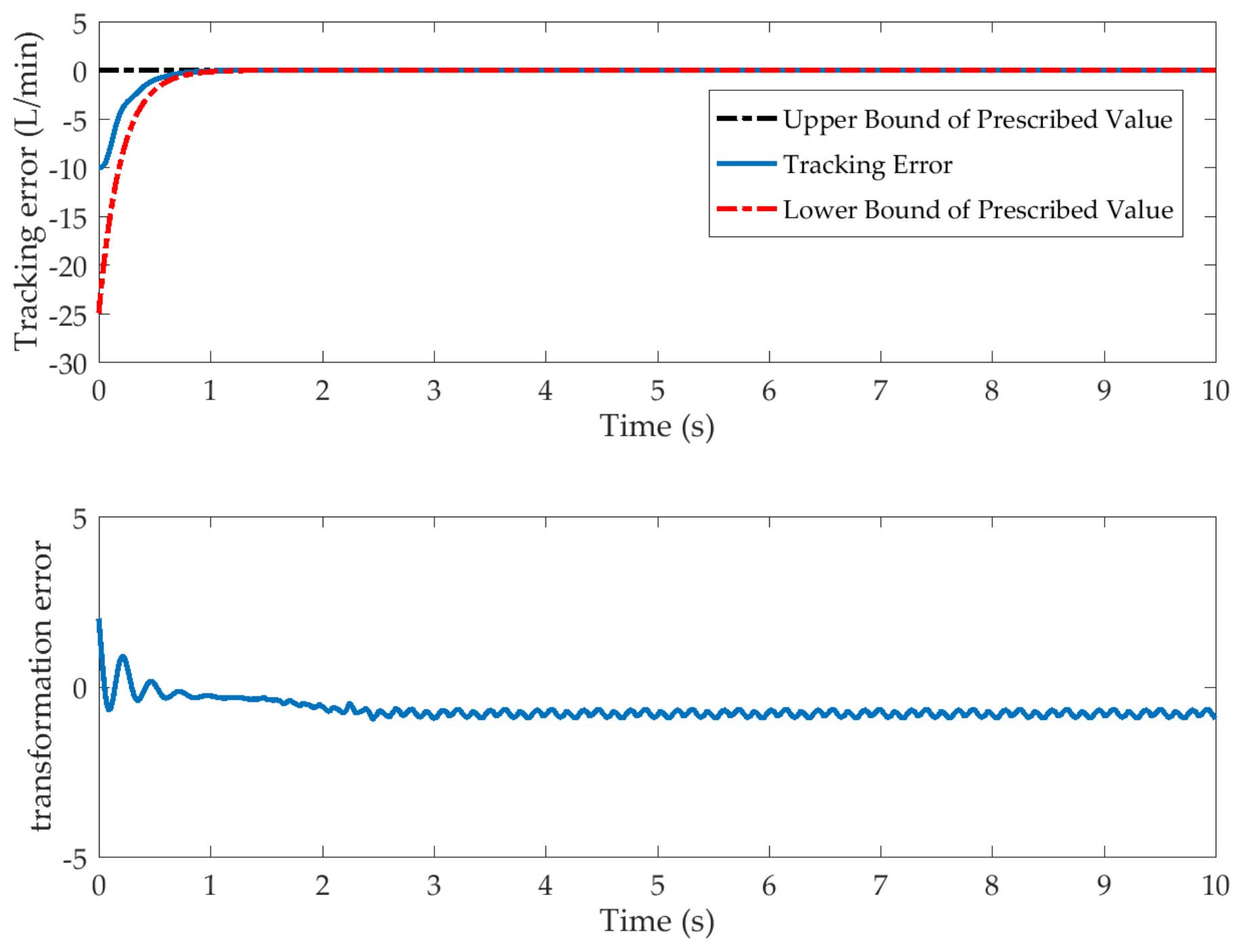
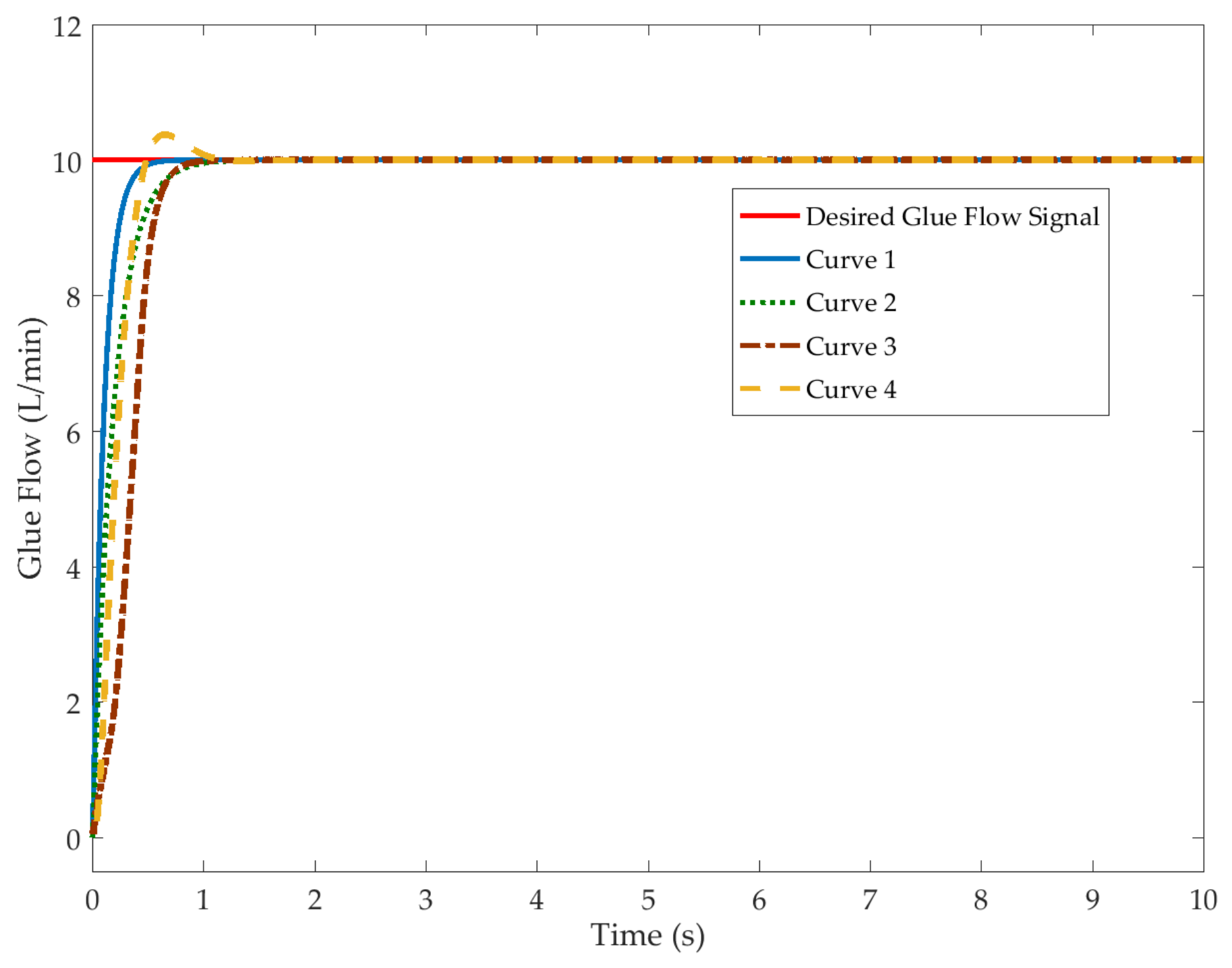
4.2. Simulation Analysis

The motivation of this section is to make the output of the established system track the desired glue flow signal, which is the input to the controlled system. For example, when glue needs to be applied to the particlebaord at the speed of 10 L/min, the output of the system should track it as quickly and smoothly as possible.

The parameters in the controller were chosen by the trial and error method. A set of simulation results is shown in Figure 8 to demonstrate this process. Considering that the PID method has a stable control performance in many applications, in the process of controller parameter selection, the PID control performance was taken as the expected goal for parameter design. Firstly, a set of PID parameters was selected as the control performance goal shown as Curve 1; then, the sliding-mode dynamic surface controller was designed to approach Curve 2 by constantly changing the design parameters, and Curves 3.4 were obtained; curve 4 means that overshoot occurs when achieving the fast tracking signal, which is not allowed; the prescribed performance method was added on the basis of sliding-mode dynamic surface shown as Curve 1, and it can realize a faster tracking signal than PID due to PPC being able to control the transient performance, including the convergence speed. It should be explained that the results shown in the figure only selected several curves representing the parameters’ choosing process.

Figure 9 shows the input of the system. It can be seen that the input curve is smoother when the tanh function is used as the switching term where $\mu =0.01$. Compared with the switching term using a sign function, it can be seen that the chattering is weakened.

Case 1: In order to verify the effects of the prescribed performance control method without extended state observers, we compared it with an adaptive dynamic surface control, inspired by [50], in order to demonstrate that it has superior transient and steady-state performance in the controlled system.

Due to the tracking error $e\left(0\right)=x_1\left(0\right)-y_d=-10$ L/min, the parameters of the performance function were designed as follows:

$${\rho }_0=25 \mathrm{L}/\min ,{\rho }_{\infty }=1\times {10}^{-4} \mathrm{L}/\min ,\nu =55.$$

The tuning parameters for the proposed controller were set as: $k_1=30$, $k_2=120$, $k_3=150$, $\eta =[3,3,1]$, $\zeta =[2,1]$, ${\omega }_{e}1={\omega }_{e}2=1\times {10}^{-2}$, and $\gamma =5$. Furthermore, the time constant in the first-order filter was set to $\tau =0.001$.

The simulation results are shown in Figure 10, Figure 11 and Figure 12. In Figure 10, Controller 1 represents the method shown in [50] without the interval type-2 fuzzy neural networks. Controller 2 represents the DSC method. It can be seen that the tracking curve was able to quickly and accurately track the desired flow signal. Compared with adaptive DSC, it had a higher convergence speed in the transient stage without overshooting, reflecting the effect of introducing the performance function.

In order to further verify the effect of the performance function, the inequality in Equations (13) and (16), which represent the preset performance control, is shown in Figure 11. It can be seen that the flow tracking error and convergence speed were always within the specified range without overshooting, which indicates accurate application of the prescribed amount of glue; this is an important and representative embodiment of the process. Although the transformation error of the system does not converge to zero and the jitter is obvious, it is still stable in the field near zero. This does not affect the preset performance control algorithm, which still plays a significant role in the process of accurate and rapid control of the system.

The virtual control input and output of the first-order filter in the dynamic surface control is shown in Figure 12. As the results showed, the output curve is relatively smooth, and the virtual input variation error after passing through the first-order filter in the second subsystem can be maintained in a relatively small field, which proves that it ha a good ability to calculate the virtual input derivative.

Case 2: To illustrate the effectiveness of the two extended state observers, we used the sliding-mode dynamic surface control scheme based on the ESOs’ combined prescribed performance.

The tuning parameters of the proposed controller were chosen as $k_1=50$, $k_2=200$, $k_3=130$, $\eta =[3,3,1]$, $\zeta =[2,1]$, ${\omega }_{e}1={\omega }_{e}2=1\times {10}^{-2}$, $\gamma =1000$; the time constant in the first-order filter was chosen as $\tau =0.001$. The simulation results are shown in Figure 13, Figure 14, Figure 15 and Figure 16.

The time response of glue flow tracking is shown in Figure 13. Controller a represents the improved active disturbance rejection control method based on the neural network state observer shown in [51]. Controller b represents the high-gain observer-based sliding-mode dynamic surface control method. Controller c represents the DSC method. Controller d represents the SMC method.

Controller a represents the ADRC method, which is aimed at practical engineering combined with the neural network observer to observe the external disturbance. Controller b represents the sliding-mode dynamic surface control based on a single high-gain observer without prescribed performance. The comparison between the proposed controller and Controllers c and d shows that the combination of the two methods can achieve better control performance. It can be seen that the proposed controller can track the desired flow signal accurately and quickly by the comparison.

In order to prove the effectiveness of the two extended state observers, the results are shown in Figure 14. The uncertainties $\Delta g=0$ and $\Delta f=0$ facilitated the analysis, and the mismatched/matched disturbances were chosen as compound sinusoidal signals. It can be seen, from the results, that the designed observers were able to accurately approximate the matched and mismatched disturbances of the system, thus making it able to effectively compensate for the external disturbances in the feed-forward channel, in order to enhance the stability and robustness of the system.

In Figure 15, uncertainties are still not considered, but the mismatched/matched disturbances were chosen to be random noise signals, in order to simulate actual working conditions. The results showed that the ESOs still had excellent approximation performance for the mismatched/matched disturbances, even when the performance function was added and the disturbance were random noise, which caused the complexity of the controller to increase.

The two cases above only considered uncertain linear disturbances, including mismatched/matched disturbances. Therefore, we set the uncertainties $\Delta g\ne 0$ and $\Delta f\ne 0$, in order to verify the superior robustness of the proposed method. Figure 16 reflects the time response of the ESOs in the compound controller. Even when the uncertainty functions were added, the observer could still approximate the uncertainties.

5. Conclusions

In this paper, a robust compound performance control scheme based on ESOs was proposed for the problem of controlling the glue-dosing speed in a particleboard glue-dosing system. It was shown to be able to achieve accurate and rapid control performance for the tracking of the glue flow in the presence of external interferences and unknown uncertainties. Mismatched/matched uncertainties were approximated and compensated in a feed-forward way through the design of ESOs, which effectively enhanced the robustness of the control system. A new error transformation function was introduced, and a prescribed performance control method was used, in order to keep the tracking error and tracking speed within a small, specified range, ensuring the transient performance of the system. In order to solve the problem that the observer could not fully approach the uncertainties in order to further improve the performance, the sliding-mode dynamic surface control method was introduced, and the computational burden of the control scheme was reduced through the introduction of a first-order filter. The results demonstrated that the proposed method has a fast convergence speed and a small steady-state convergence error, both of which satisfy the expectations for the tracking effect, indicating that the glue flow can be accurately controlled.

References

1. Oshaba, A.S.; Ali, E.S.; Abd Elazim, S.M. PI controller design via ABC algorithm for MPPT of PV system supplying DC motor-pump load. Electr. Eng. 2017, 99, 505–518. [Google Scholar] [CrossRef]
2. Helian, B.; Chen, Z.; Yao, B. Precision Motion Control of a Servomotor-Pump Direct-Drive Electrohydraulic System with a Nonlinear Pump Flow Mapping. IEEE Trans. Ind. Electron. 2020, 67, 8638–8648. [Google Scholar] [CrossRef]
3. Gherbi, A.D.; Arab, A.H.; Salhi, H. Improvement and validation of PV motor-pump model for PV pumping system performance analysis. Sol. Energy 2017, 144, 310–320. [Google Scholar] [CrossRef]
4. Wang, S.; Tao, L.; Chen, Q.; Na, J.; Ren, X. USDE-Based Sliding Mode Control for Servo Mechanisms With Unknown System Dynamics. IEEE/Asme Trans. Mechatron. 2020, 25, 1056–1066. [Google Scholar] [CrossRef]
5. Chalanga, A.; Kamal, S.; Fridman, L.; Bandyopadhyay, B.; Moreno, J. How to Implement Super-Twisting Controller based on Sliding Mode Observer? In Proceedings of the 13th International Work- shop on Variable Structure Systems, Nantes, France, 29 June–2 July 2014. [Google Scholar] [CrossRef]
6. Chalanga, A.; Kamal, S.; Fridman, L.; Bandyopadhyay, B.; Moreno, J. Implementation of Super-Twisting Control: Super-Twisting and Higher Order Sliding Mode Observer Based Approaches. IEEE Trans. Ind. Electron. 2015, 63, 3677–3685. [Google Scholar] [CrossRef]
7. Meguenni, K.Z.; Tahar, M.; Benhadria, M.R.; Bestaoui, Y. Fuzzy integral sliding-mode based on backstepping control synthesis for an autonomous helicopter. Proc. Inst. Mech. Eng. Part G J. Aerosp. Eng. 2013, 227, 751–765. [Google Scholar] [CrossRef]
8. Wu, M.; Zhu, H. Backstepping control of three-pole radial hybrid magnetic bearing. IET Electr. Power Appl. 2020, 14, 1405–1411. [Google Scholar] [CrossRef]
9. Sun, K.; Mou, S.; Qiu, J.; Wang, T.; Gao, H. Adaptive Fuzzy Control for Nontriangular Structural Stochastic Switched Nonlinear Systems With Full State Constraints. IEEE Trans. Fuzzy Syst. 2019, 27, 1587–1601. [Google Scholar] [CrossRef]
10. Shao, X.; Hu, Q.; Shi, Y. Adaptive Pose Control for Spacecraft Proximity Operations with Prescribed Performance Under Spatial Motion Constraints. IEEE Trans. Control. Syst. Technol. 2020, 29, 1405–1419. [Google Scholar] [CrossRef]
11. Liu, Y.J.; Tong, S. Barrier Lyapunov functions for Nussbaum gain adaptive control of full state constrained nonlinear systems. Automatica 2017, 76, 143–152. [Google Scholar] [CrossRef]
12. Preitl, S.; Precup, R.E.; János, F.; Bede, B. Iterative Feedback Tuning in Fuzzy Control Systems. Theory and Applications. Acta Polytech. Hung. 2006, 3, 81–96. [Google Scholar]
13. Turnip, A.; Panggabean, J.H. Hybrid controller design based magneto-rheological damper lookup table for quarter car suspension. Int. J. Artif. Intell. 2020, 18, 193–206. [Google Scholar]
14. Roman, R.C.; Precup, R.E.; Petriu, E.M. Hybrid data-driven fuzzy active disturbance rejection control for tower crane systems. Eur. J. Control 2021, 58, 373–387. [Google Scholar] [CrossRef]
15. Bechlioulis, C.P.; Rovithakis, G.A. Robust Adaptive Control of Feedback Linearizable MIMO Nonlinear Systems with Prescribed Performance. IEEE Trans. Autom. Control 2008, 53, 2090–2099. [Google Scholar] [CrossRef]
16. Dai, S.L.; He, S.; Lin, H.; Wang, C. Platoon Formation Control With Prescribed Performance Guarantees for USVs. IEEE Trans. Ind. Electron. 2018, 65, 4237–4246. [Google Scholar] [CrossRef]
17. Zhu, Y.; Qiao, J.; Guo, L. Adaptive Sliding Mode Disturbance Observer-Based Composite Control with Prescribed Performance of Space Manipulators for Target Capturing. IEEE Trans. Ind. Electron. 2019, 66, 1973–1983. [Google Scholar] [CrossRef]
18. Shao, X.; Hu, Q.; Shi, Y.; Jiang, B. Fault-Tolerant Prescribed Performance Attitude Tracking Control for Spacecraft Under Input Saturation. IEEE Trans. Control. Syst. Technol. 2020, 28, 574–582. [Google Scholar] [CrossRef]
19. Zheng, Z.; Feroskhan, M. Path Following of a Surface Vessel With Prescribed Performance in the Presence of Input Saturation and External Disturbances. IEEE/Asme Trans. Mechatron. 2017, 22, 2564–2575. [Google Scholar] [CrossRef]
20. Wang, Y.; Hu, J.; Zheng, Y. Improved decentralized prescribed performance control for non-affine large-scale systems with uncertain actuator nonlinearity. J. Frankl. Inst. 2019, 356, 7091–7111. [Google Scholar] [CrossRef]
21. Tooranjipour, P.; Vatankhah, R.; Arefi, M. Prescribed performance adaptive fuzzy dynamic surface control of non-affine time-varying delayed systems with unknown control directions and dead-zone input. Int. J. Adapt. Control Signal Process. 2019, 33, 1134–1156. [Google Scholar] [CrossRef]
22. Zhang, J.J.; Sun, Q.M. Prescribed performance adaptive neural output feedback dynamic surface control for a class of strict-feedback uncertain nonlinear systems with full state constraints and unmodeled dynamics. Int. J. Robust Nonlinear Control 2020, 30, 459–483. [Google Scholar] [CrossRef]
23. Tee, K.P.; Ge, S.S.; Tay, E.H. Barrier Lyapunov Functions for the control of output-constrained nonlinear systems. Automatica 2009, 45, 918–927. [Google Scholar] [CrossRef]
24. Hu, Y.A.; Li, H.Y.; Huang, H. Prescribed performance-based backstepping design for synchronization of cross-strict feedback hyperchaotic systems with uncertainties. Nonlinear Dyn. 2014, 76, 103–113. [Google Scholar] [CrossRef]
25. Jin, Z.; Zhang, W.; Liu, S.; Gu, M. Command-Filtered Backstepping Integral Sliding Mode Control with Prescribed Performance for Ship Roll Stabilization. Appl. Sci. 2019, 9, 4288. [Google Scholar] [CrossRef] [Green Version]
26. Guo, Q.; Zhang, Y.; Celler, B.G.; Su, S.W. Neural Adaptive Backstepping Control of a Robotic Manipulator With Prescribed Performance Constraint. IEEE Trans. Neural Networks Learn. Syst. 2019, 30, 3572–3583. [Google Scholar] [CrossRef]
27. Song, M.; Lin, Y. Modified adaptive backstepping design method for linear systems. IET Control Theory Appl. 2012, 6, 1137–1144. [Google Scholar] [CrossRef]
28. Dai, J.; Ren, B.; Zhong, Q.C. Uncertainty and Disturbance Estimator-Based Backstepping Control for Nonlinear Systems With Mismatched Uncertainties and Disturbances. J. Dyn. Syst. Meas. Control 2018, 140, 121005. [Google Scholar] [CrossRef] [Green Version]
29. Swaroop, D.; Hedrick, J.K.; Yip, P.P.; Gerdes, J.C. Dynamic surface control for a class of nonlinear systems. IEEE Trans. Autom. Control 2000, 45, 1893–1899. [Google Scholar] [CrossRef] [Green Version]
30. Li, J.; Du, J.; Hu, X. Robust adaptive prescribed performance control for dynamic positioning of ships under unknown disturbances and input constraints. Ocean Eng. 2020, 206, 107254. [Google Scholar] [CrossRef]
31. Guo, Q.; Liu, Y.; Jiang, D.; Wang, Q.; Xiong, W.; Liu, J.; Li, X. Prescribed Performance Constraint Regulation of Electrohydraulic Control Based on Backstepping with Dynamic Surface. Appl. Sci. 2018, 8, 776. [Google Scholar] [CrossRef] [Green Version]
32. Chen, L. Asymmetric prescribed performance-barrier Lyapunov function for the adaptive dynamic surface control of unknown pure-feedback nonlinear switched systems with output constraints. Int. J. Adapt. Control Signal Process. 2018, 32, 1417–1439. [Google Scholar] [CrossRef]
33. Jia, F.; Wang, X.; Zhou, X. Robust adaptive prescribed performance control for a class of nonlinear pure-feedback systems. Int. J. Robust Nonlinear Control 2019, 29, 3971–3987. [Google Scholar] [CrossRef]
34. Lei, D.; Wang, T.; Cao, D.; Fei, J. Adaptive Dynamic Surface Control of MEMS Gyroscope Sensor Using Fuzzy Compensator. IEEE Access 2016, 4, 4148–4154. [Google Scholar] [CrossRef]
35. Han, S.I.; Lee, J.M. Adaptive dynamic surface control with sliding-mode control and RWNN for robust positioning of a linear motion stage. Mechatronics 2012, 22, 222–238. [Google Scholar] [CrossRef]
36. Keighobadi, J.; Hosseini-Pishrobat, M.; Faraji, J. Adaptive neural dynamic surface control of mechanical systems using integral terminal sliding-mode. Neurocomputing 2020, 379, 141–151. [Google Scholar] [CrossRef]
37. Jing, C.; Xu, H.; Niu, X. Adaptive sliding-mode disturbance rejection control with prescribed performance for robotic manipulators. ISA Trans. 2019, 91, 41–51. [Google Scholar] [CrossRef] [PubMed]
38. Zhang, W.; Xu, D.; Jiang, B.; Pan, T. Prescribed performance based model-free adaptive sliding-mode constrained control for a class of nonlinear systems. Inf. Sci. 2021, 544, 97–116. [Google Scholar] [CrossRef]
39. Luenberger, D.G. Observing the State of a Linear System. IEEE Trans. Mil. Electron. 1964, 8, 74–80. [Google Scholar] [CrossRef]
40. Ma, H.; Li, H.; Liang, H.; Dong, G. Adaptive Fuzzy Event-Triggered Control for Stochastic Nonlinear Systems With Full State Constraints and Actuator Faults. IEEE Trans. Fuzzy Syst. 2019, 27, 2242–2254. [Google Scholar] [CrossRef]
41. Zhang, X.; Ding, F.; Xu, L.; Yang, E. State filtering-based least squares parameter estimation for bilinear systems using the hierarchical identification principle. IET Control Theory Appl. 2018, 12, 1704–1713. [Google Scholar] [CrossRef] [Green Version]
42. Cui, R.; Chen, L.; Yang, C.; Chen, M. Extended State Observer-Based Integral Sliding Mode Control for an Underwater Robot With Unknown Disturbances and Uncertain Nonlinearities. IEEE Trans. Ind. Electron. 2017, 64, 6785–6795. [Google Scholar] [CrossRef] [Green Version]
43. Wang, L.; Xi, J.; He, M.; Liu, G. Robust time-varying formation design for multiagent systems with disturbances: Extended-state-observer method. Int. J. Robust Nonlinear Control 2020, 30, 2796–2808. [Google Scholar] [CrossRef] [Green Version]
44. Yao, J.; Deng, W. Active Disturbance Rejection Adaptive Control of Hydraulic Servo Systems. IEEE Trans. Ind. Electron. 2017, 64, 8023–8032. [Google Scholar] [CrossRef]
45. Hamidat, A.; Benyoucef, B. Mathematic models of photovoltaic motor-pump systems. Renew. Energy 2008, 33, 933–942. [Google Scholar] [CrossRef]
46. Singh, B.; Putta Swamy, C.L.; Singh, B.P. Analysis and development of a low-cost permanent magnet brushless DC motor drive for PV-array fed water pumping system. Sol. Energy Mater. Sol. Cells 1998, 51, 55–67. [Google Scholar] [CrossRef]
47. Tee, K.P.; Ren, B.; Ge, S.S. Control of nonlinear systems with time-varying output constraints. Automatica 2011, 47, 2511–2516. [Google Scholar] [CrossRef]
48. Ren, B.B.; Ge, S.S.; Tee, K.P.; Lee, T.H. Adaptive Neural Control for Output Feedback Nonlinear Systems Using a Barrier Lyapunov Function. IEEE Trans. Neural Netw. 2010, 21, 1339–1345. [Google Scholar] [CrossRef]
49. Mien, V.; Mavrovouniotis, M.; Ge, S.S. An Adaptive Backstepping Nonsingular Fast Terminal Sliding Mode Control for Robust Fault Tolerant Control of Robot Manipulators. IEEE Trans. Syst. Man Cybern. Syst. 2019, 49, 1448–1458. [Google Scholar] [CrossRef] [Green Version]
50. Chang, Y.H.; Chan, W.S. Adaptive Dynamic Surface Control for Uncertain Nonlinear Systems With Interval Type-2 Fuzzy Neural Networks. IEEE Trans. Cybern. 2014, 44, 293–304. [Google Scholar] [CrossRef]
51. Wang, P.; Zhang, C.; Zhu, L.; Wang, C. The Research of Improved Active Disturbance Rejection Control Algorithm for Particleboard Glue System Based on Neural Network State Observer. Algorithms 2019, 12, 259. [Google Scholar] [CrossRef] [Green Version]
Figure 1. Glue preparation subprocess of the particleboard glue-dosing process: 1. curing agent; 2. waterproofing agent; 3. curing buffer agent; 4. water; 5. liquid level detector; 6. quantitative barrel; 7. electronically controlled throttle valve; 8. feeding tube; 9. cylinder; 10. ball valve; 11. blanking tube; 12. agitator; 13. glue mixing case.
Actuators 10 00282 g001
Figure 2. Glue-dosing subprocess of the particleboard glue-dosing process.
Actuators 10 00282 g002
Figure 3. GMD-A-type particleboard glue-dosing simulation system.
Actuators 10 00282 g003
Figure 4. Glue pump motor.
Actuators 10 00282 g004
Figure 5. Schematic diagram of the glue-dosing process.
Actuators 10 00282 g005
Figure 6. Time response of the hyperbolic tangent function.
Actuators 10 00282 g006
Figure 7. The configuration of the compound controller.
Actuators 10 00282 g007
Figure 8. Time response of glue flow tracking.
Actuators 10 00282 g008
Figure 9. Time response of control input.
Actuators 10 00282 g009
Figure 10. Time response of the glue flow tracking.
Actuators 10 00282 g010
Figure 11. Time response of the performance function.
Actuators 10 00282 g011
Figure 12. Time response of the first-order filter.
Actuators 10 00282 g012
Figure 13. Time response of glue flow tracking.
Actuators 10 00282 g013
Figure 14. Time response of the 2 ESOs in the controller.
Actuators 10 00282 g014
Figure 15. Time response of the ESOs.
Actuators 10 00282 g015
Figure 16. Time response of the ESOs.
Actuators 10 00282 g016