Article

Event-Based, Intermittent, Discrete Adaptive Control for Speed Regulation of Artificial Legs

by
Salvador Echeveste
,
Ernesto Hernandez-Hinojosa
and
Pranav A. Bhounsule
*
Department of Mechanical and Industrial Engineering, University of Illinois at Chicago, 842 W. Taylor St., Chicago, IL 60607, USA
*
Author to whom correspondence should be addressed.
Actuators 2021, 10(10), 264; https://doi.org/10.3390/act10100264
Submission received: 2 September 2021 / Revised: 2 October 2021 / Accepted: 8 October 2021 / Published: 12 October 2021

Abstract

:
For artificial legs that are used in legged robots, exoskeletons, and prostheses, it suffices to achieve velocity regulation at a few key instants of swing rather than tight trajectory tracking. Here, we advertise an event-based, intermittent, discrete controller to enable set-point regulation for problems that are traditionally posed as trajectory following. We measure the system state at prior-chosen instants known as events (e.g., vertically downward position), and we turn on the controller intermittently based on the regulation errors at the set point. The controller is truly discrete, as these measurements and controls occur at the time scale of the system to be controlled. To enable set-point regulation in the presence of uncertainty, we use the errors to tune the model parameters. We demonstrate the method in the velocity control of an artificial leg, a simple pendulum, with up to 50% mass uncertainty. Starting with a 100% regulation error, we achieve velocity regulation of up to 10% in about five swings with only one measurement per swing.

1. Introduction

For legged robots, powered prosthetics, and powered exoskeletons to be successful, one needs appropriate swing-leg control in the presence of model uncertainty (e.g., uncertainty in inertia and damping). This is typically achieved by setting up a reference trajectory for the swing leg and then using a high-gain feedback controller to track the reference trajectory. However, it is worth noting that it is sufficient for the swing leg to achieve a set velocity at a given instant of the swing instead of tracking a series of reference points at multiple points in the swing. In this paper, we achieve swing-leg control by tracking a set point, the velocity at a chosen instant, instead of a reference trajectory. This alternate formulation is simpler because it requires a few measurements (typically one or two per step), few computations (offline design of feedback gain), and low-bandwidth control (typically of the order of 1 or 2 Hz). We call such a control event-based, intermittent, discrete control.
Another challenge, especially with powered prosthetics and exoskeletons, is that the parameters of the control need to be tuned for a specific individual based on the dynamics of their able leg. Although a high-gain-tracking controller may achieve desired outcomes, it might amplify the sensor noise, leading to instability. Alternately, careful tuning of the feedback gains may achieve acceptable performance, but such hand-tuning is potentially time consuming. A more customizable method is to have an adaptive controller that self-tunes itself using on-board measurements. In this paper, we further develop an adaptive control layer to enable automatic tuning of the discrete controller.
We present an event-based, intermittent, discrete adaptive controller for controlling systems using low-bandwidth measurements and control while achieving an appropriate performance index. We demonstrate results on the benchmark problem of swinging of a pendulum in a simulation and experiments. In the future, we expect to apply the control method on a legged robot and a hip exoskeleton.

2. Background and Related Work

One of the earliest hypotheses was that the human leg swing is ballistic, i.e., there is no active control during the leg swing [1,2]. However, later works found that a pure ballistic swing underestimated the swing time and step length and did not accurately predict the ground reaction forces [3]. Later works found that the swing leg is not totally passive, as it entails a metabolic cost and there is muscle activity for initiation and propagation of the swing leg [4].
Active control of exoskeletons and prostheses relies on tracking a reference motion using a high-gain feedback controller [5] or just loose tracking of a set of reference points in the swing [6]. In the latter approach, one divides the swing phase into a series of phases. In each phase, there are set points that are loosely tracked using a low-gain proportional–derivative controller. A more extreme approach is to tune a controller once per step by using measurements obtained during the step. For example, by modulating the ankle push-off based on the average progression speed, it is possible to achieve balance control [7]. Instead of actively injecting energy, there are artificial devices that extract energy using magneto-rheological dampers to achieve swing control [8].
The ballistic swing model of humans inspired passive dynamic walking robots. Such robots can walk downhill with no external torque input or power, relying solely on the mass, inertia, and geometry of their legs [9]. However, such robots can only walk on shallow slopes, limiting them to slow speeds and short step lengths [10]. Increasing the slope increases the walking speed, but requires active control of the hip joint [11]. Alternately, to enable walking at human speed on level grounds, one needs to tune the leg frequency using either active control or a hip spring and an ankle push-off to overcome energy losses during the foot strike [12,13].
Similarly to that of exoskeletons and prostheses, the control of legged robots ranges from tight trajectory tracking to once-per-step control. The most prominent idea has been the hybrid zero-dynamics approach in which one defines a set of canonical output functions using heuristics [14], optimization [15], or human data [16]. These outputs can be tracked using a high-gain feedback controller. An alternate approach is loosely tracking distinct set points during the gait cycle using a low-gain feedback control so that the tracking is approximate [17]. A more extreme approach, the once-per-step control, is the modulation of a single control parameter (e.g., ankle push-off) during the gait cycle [18]. For hopping robots, it has been shown that control of the hop height, the forward speed, and the torso using three independent controllers can achieve highly robust running for one-, two-, and four-legged robots [19].
Adaptive control of artificial legs is achieved with tight trajectory tracking using a model reference adaptive control that tunes the controller based on tracking errors [20] or a model identification adaptive control in which the model is taught from the errors [21]. Other approaches have considered optimal control using dynamic programming [22], extremum-seeking control [23], and reinforcement-learning-based approaches [24].
The concept of tracking set points instead of trajectory tracking has similarities with past work done on controlling lightly damped systems, such as point-to-point movement of a crane using a hoist. One such application is the point-to-point movement of cranes using a cable hoist, where improper movement of the crane leads to unnecessary vibration of the payload at the end of the movement [25]. One method is the ‘posicast’ method, in which the input command is delayed in such a way that it causes vibration produced by the pre-delay input signal [26,27]. Another method is called ‘input shaping’ or command shaping, in which two impulses that are separated in time are convolved with the input command. The timing of the impulse is so chosen that the vibration induced by the first one is exactly cancelled by the second one, leading to cancellation of the vibration [28,29]. Both methods—the posicast and the input shaping method—tune the feedforward command to achieve vibration suppression.
The method proposed in this paper is closest to ‘intermittent control’ [30]. Here, the control is made up of the multiplication of a time-based part and a basis function. The time-based part is optimized for the steady-state response or feedforward response, while the basis function is tuned based on measurement errors. The control is intermittent because the basis function is not continuously tuned, but only based on errors at events in the control cycle. Intermittent control has been used for inverted pendulum control [31] and to explain humans balancing a stick on their hands [32], as well as human standing balance [33].
In this paper, we present the event-based, intermittent, discrete adaptive controller design. Here, we measure the system state during events in the motion (e.g., vertically downward position for a pendulum swing). Based on these measurements, we compute control parameters that turn the control ON intermittently (e.g., torque is ON for a few milliseconds during the pendulum swing). The controller is discrete in the sense that the time intervals between measurements are typical of the order of the natural frequency of the system. Then, we add an adaptive controller that tunes the control parameters using sensor measurements. This paper extends our event-based, intermittent, discrete controller design, which is similar to the intermittent control approach [34], to adaptive control, and this is the main novelty of the paper.
The flow of the paper is as follows. We present the methods for event-based, intermittent control and then extend them to perform adaptive control in Section 3. Next, we present results on simulations and hardware in Section 4. The discussion follows in Section 5, and this is followed by the conclusion in Section 6.

3. Methods

3.1. Overview of Control

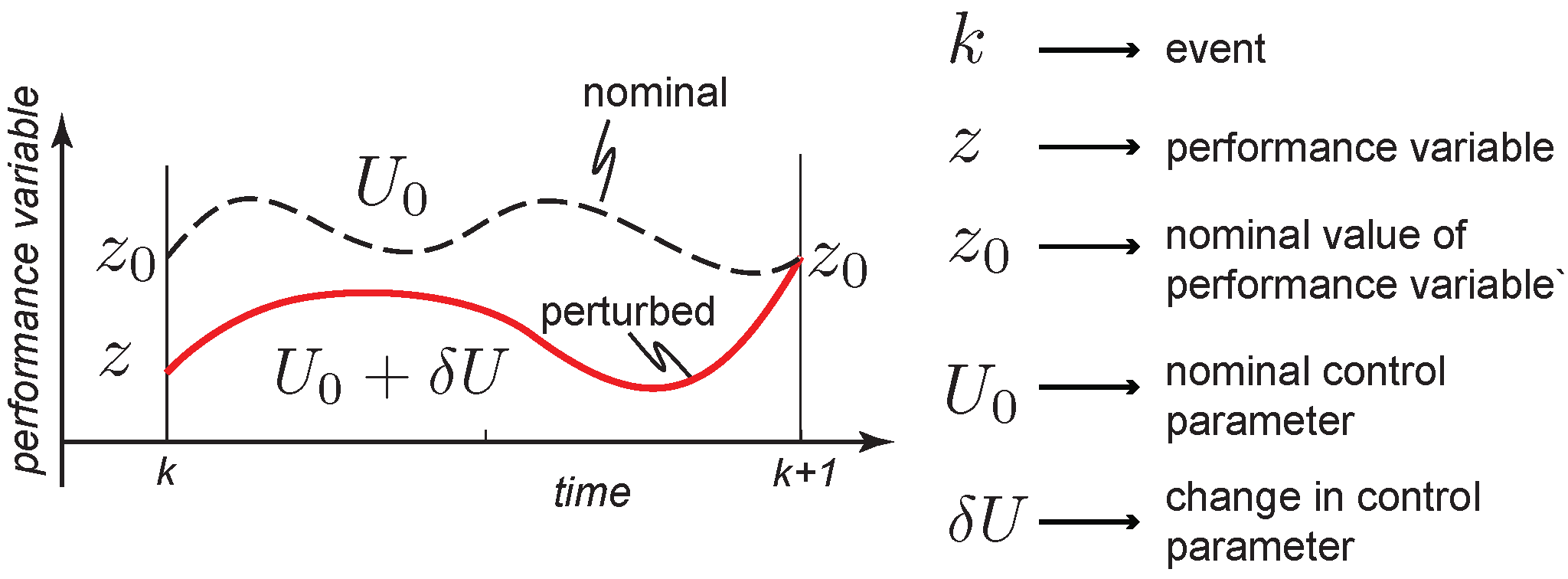
Figure 1 summarizes the control idea. We show the nominal motion of the system using a black dashed line. This corresponds to the use of the nominal control parameter U 0 . Since we are specifically looking at periodic motion, the performance variable z, which is a function of the state, is z 0 at the instant k and k + 1 . When the system deviates from the nominal, the state at section k is z. Now, we have to find the correction to the nominal control parameter δ U such that the new control parameter U 0 + δ U brings the performance variable close to z 0 at the event k + 1 .
There are few things in the controller that differ from traditional feedback control. First, the time interval between the events k and k + 1 is typically at the order of the natural time constant of the system and not at the bandwidth provided by the computing and hardware of the system. Second, we take measurements of the system z and make control corrections δ U at key instances, again at the order of the natural frequency of the system. Finally, the controller regulates the system to the performance index—here, z = z 0 —at key instants instead of tight trajectory tracking. We now describe the specifics of the controller.

3.2. Event-Based, Intermittent, Discrete Control

Let the state of the system be x ( t ) , the control be u ( t ) , and the continuous system dynamics be defined by F with x ˙ = F ( x , u ) . Let the control be parameterized by the free variable U (e.g., gain, amplitude, set point) such that u ( t ) = f ( t , x , U ) , where f is a function of state, time, or a combination of both. Assume that there is a nominal control u 0 ( t ) = f ( x , t , U 0 ) that leads to some nominal motion for the states x 0 ( t ) .
In the problems considered in this paper, we are not interested in tight tracking of the reference trajectory x 0 ( t ) . Rather, we want to track a suitable performance variable z ( x ) (e.g., energy, cartesian position, joint angle) at some state-based or time-based event (e.g., t = constant , g ( x ) = constant , where g is some nonlinear function) such that z = z 0 at some instant. The overall outlook of the event-based control paradigm is as follows. We measure the system state at some state-based or time-based event. Let us assume that the state has deviated from its nominal value, δ x = ( x x 0 ) . The goal then is to find the differential control parameters δ U = U U 0 such that we minimize the deviation δ z = ( z z 0 ) . The control is intermittent, as we set the free parameter at the events using the measurement and regulation error.
We can linearize the system at the nominal value of the performance index z between the events k and k + 1 to get
δ z ( k + 1 ) = a δ z ( k ) + b δ U ( k )
where z R and U R . since the goal is to reduce δ z = z z 0 = 0 . We achieve this in a single measurement and control cycle by choosing δ U ( k ) = a b δ z ( k ) , assuming b 0 . Such a control that achieves full correction of disturbances in a single step is known as a one-step deadbeat controller (e.g., see [35], p. 201).

3.3. Adaptive Control

In the previous section, we showed how to choose a control if the model F of the system is fully known. However, there may be modeling errors; as such, we may only know an imperfect model x ˙ = F ^ ( x , u ) . In this case, our estimates for the linearized parameters are a ^ and b ^ . Thus, we will have an error
e ( k ) = δ z ( k + 1 ) a ^ δ z ( k ) b ^ δ U ( k ) = δ z ( k + 1 ) X T ( k ) w ^
where w ^ = a ^ , b ^ T are weights and X ( k ) = δ z ( k ) , δ U ( k ) T is the regressor. We now define a cost function
J ( w ^ ( k ) ) = 1 2 e 2 ( k ) n 2 ( k )
where n = ϵ + X T ( k ) X ( k ) is the normalizing factor with a user-chosen small positive constant, ϵ > 0 .
The update in the weight w ^ can now be obtained by gradient descent:
w ^ ( k + 1 ) = w ^ ( k ) λ J w ^ ( k ) = w ^ ( k ) λ J e ( k ) e ( k ) w ^ ( k ) = w ^ ( k ) + λ e ( k ) n 2 ( k ) X ( k )
where 0 < λ < 2 is a user-tuned gain. This can also be a function of iteration, i.e., λ ( k ) . It can be shown that the adaptive law above guarantees that the weights w ^ and error e are bounded and l i m t e = 0 (e.g., see [36], Chapter 3).

3.4. Control of a Pendulum

We demonstrate the event-based, intermittent, discrete adaptive control for velocity control of a pendulum. First, we describe the model in continuous time, and then we describe the discrete version, followed by adaptive control.

3.4.1. Model

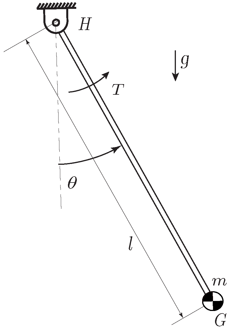
The pendulum is shown in Figure 2. The equation of motion is given by
m 2 θ ¨ + c θ ˙ + m g sin ( θ ) = T
where the mass is m, damping is c, length is , gravity is g, torque is T, and angle is θ (counter-clockwise is positive). This can be written in state-space form as
x ˙ 1 = x 2 x ˙ 2 = c m 2 x 1 + g sin ( x 1 ) 1 m 2 u
where x 1 = θ , x 2 = θ ˙ , and u = T . Our model is inaccurate, as we have not accounted for the inertia and we have used an approximate friction model.

3.4.2. Discrete-Time Model

To obtain the discrete-time model, we choose our performance variable to be energy. Thus, z = E = 0.5 m 2 x 2 2 + m g ( 1 cos ( x 1 ) ) . We measure and regulate the system energy at x 1 = θ 1 = 0 . We use a constant torque u = T = U for t s sec.
Assuming a baseline model, we first use non-linear root solving to find the control input U 0 that leads to a steady oscillation with energy E 0 for the nominal model. Thereafter, by using finite difference, we can find the constants a ^ and b ^ to obtain the discrete state equation
δ E ( k + 1 ) = a ^ δ E ( k ) + b ^ δ U ( k ) = w ( k ) T X ( k )
where δ E = E E 0 , δ U = U U 0 , w = a ^ , b ^ T , and X ( k ) = δ E ( k ) , δ U ( k ) T .
The adaptive control law may be obtained from Equation (4) as follows.
a ^ ( k + 1 ) = a ^ ( k ) + λ a e ( k ) n 2 ( k ) δ E ( k ) + f 1 ( k )
b ^ ( k + 1 ) = b ^ ( k ) + λ b e ( k ) n 2 ( k ) δ U ( k ) + f 2 ( k )
where f 1 ( k ) and f 2 ( k ) are the projection signals to keep the parameters a ^ and b ^ bounded, 0 a ^ l a ^ a ^ u and a ^ ( 0 ) a ^ l , a ^ u , and 0 b ^ l b ^ b ^ u and b ^ ( 0 ) b ^ l , b ^ u .
f 1 ( k ) = 0 , h 1 ( k ) a ^ l , a ^ u , a ^ u h 1 ( k ) h 1 ( k ) > a ^ u , a ^ l h 1 ( k ) h 1 ( k ) < a ^ l ,
f 2 ( k ) = 0 , h 2 ( k ) b ^ l , b ^ u , b ^ u h 2 ( k ) h 2 ( k ) > b ^ u , b ^ l h 2 ( k ) h 2 ( k ) < b ^ l ,
where h 1 ( k ) = a ^ ( k ) + λ a e ( k ) n 2 ( k ) δ E ( k ) and h 2 ( k ) = b ^ ( k ) + λ b e ( k ) n 2 ( k ) δ U ( k ) [36].

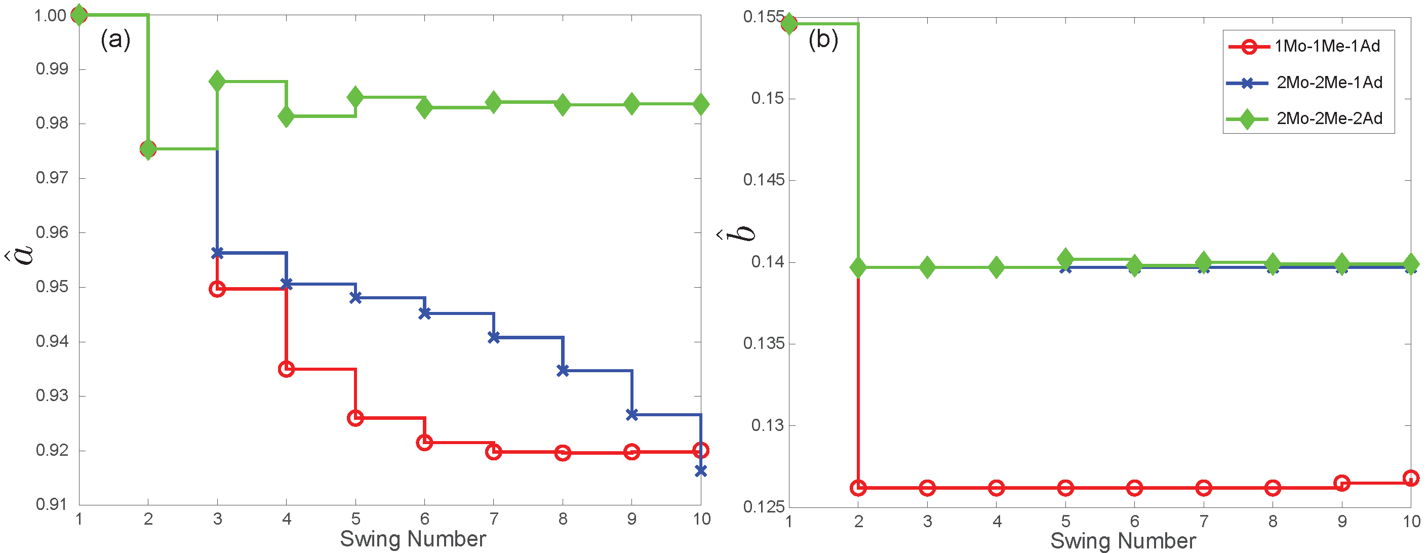
3.5. Linearized Models and Adaptations per Swing

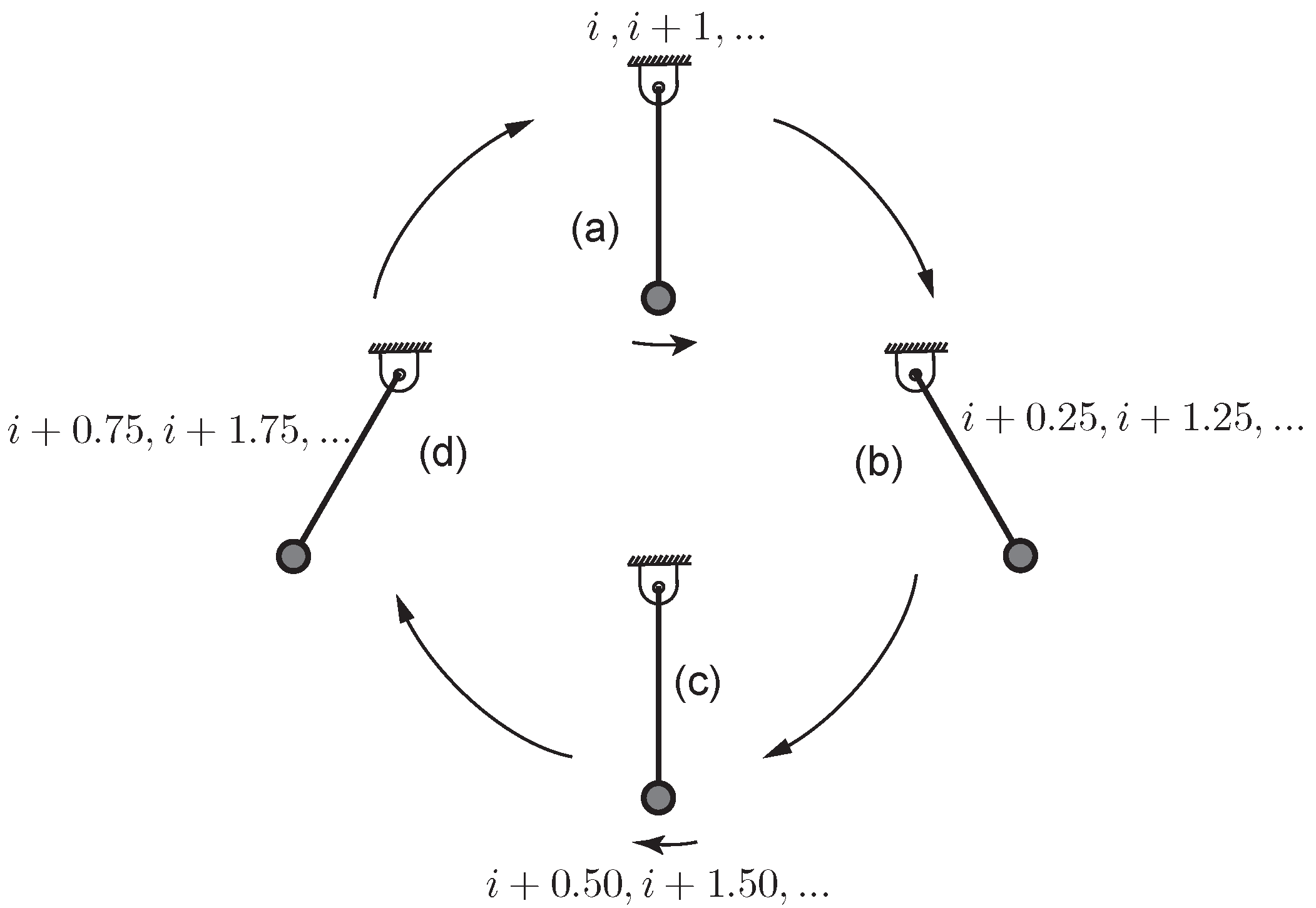
Figure 3 shows one complete swing of the pendulum. The pendulum at section i and i + 0.5 is in the vertical downward position, and at the instance i + 0.25 and i + 0.75 , it is in the extreme position. We develop three linearized models as follows. We have three different models that differ in the location of the sections and in the number of measurements and corrections made per section.

3.5.1. One Model/One Measurement/One Adaptation (1Mo-1Me-1Ad) per Period

Here, we have one model in one swing period (see Figure 3).
δ E ( i + 1 ) = a ^ 1 δ E ( i ) + b ^ 1 δ U ( i )
We measure the system energy once: when the pendulum is in the vertically downward position and moving to the right (see Figure 3a). We use this measurement to adapt the model a ^ 1 and b ^ 1 using Equations (8) and (9). Thus, we have one model, one measurement, and one adaptation per swing.

3.5.2. Two Models/Two Measurements/One Adaptation (2Mo-2Me-1Ad) per Period

Here, we have two models in one swing period (see Figure 3).
δ E ( i + 0.5 ) = a ^ 2 δ E ( i ) + b ^ 2 δ U ( i ) δ E ( i + 1 ) = a ^ 3 δ E ( i + 0.5 ) + b ^ 3 δ U ( i + 0.5 )
We measure the system energy twice: when the pendulum is in the vertically downward position and moving to the right and left (see Figure 3a,c). We use these two measurements to adapt the model a ^ 2 , a ^ 3 , b ^ 2 , and b ^ 3 using Equations (8) and (9). Thus, we have two models, two measurements, and one adaptation per model per swing.

3.5.3. Two Models/Two Measurements/Two Adaptations (2Mo-2Me-2Ad) per Period

Here, we have two models in one swing period (see Figure 3). This is done by exploiting the symmetry in 2Mo-2Me-1Ad by observing that a ^ 2 = a ^ 3 and b ^ 2 = b ^ 3 .
δ E ( i + 0.5 ) = a ^ 2 δ E ( i ) + b ^ 2 δ U ( i ) δ E ( i + 1 ) = a ^ 2 δ E ( i + 0.5 ) b ^ 2 δ U ( i + 0.5 )
We measure the system energy twice: when the pendulum is in the vertically downward position and moving to the right and left (see Figure 3a,c). We use this measurement to adapt the model parameters a ^ 2 and b ^ 3 twice using Equations (8) and (9). Thus, we have two models, two measurements, and two adaptations per model per swing.
We expect that adaptations using 2Mo-2Me-2Ad are at least two times faster compared to 1Mo-1Me-1Ad and 2Mo-2Me-1Ad. It is also noted that for directionally dependent model (e.g., friction), one cannot exploit the symmetry, and hence, 2Mo-2Me-2Ad could give poor results.
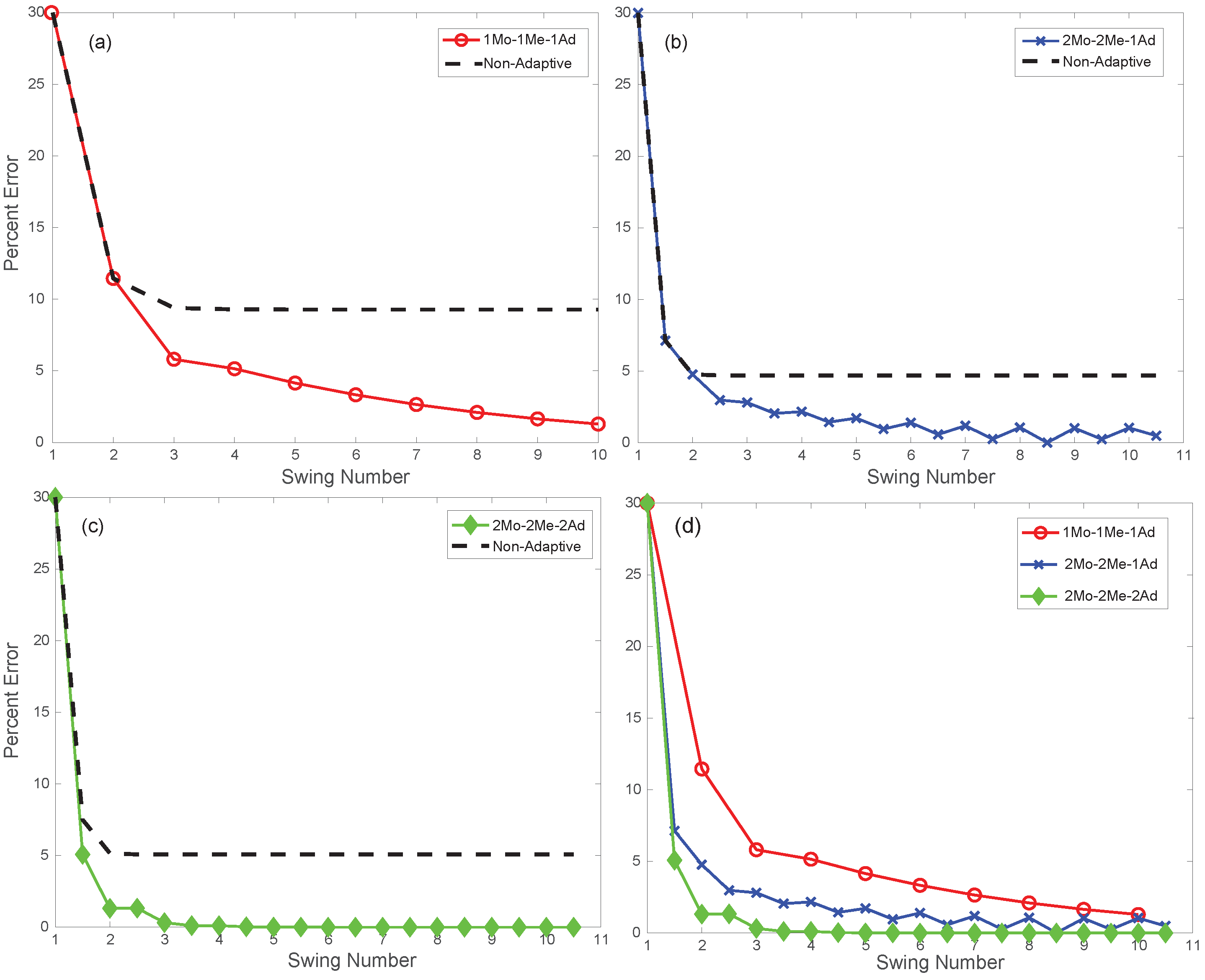
4. Results

4.1. Computer Simulations

In this section, we discuss computer simulations that were performed to validate the proposed approach. In all simulations shown here, we linearize the continuous time model shown in Equation (5). We estimate the plant parameters assuming m ^ = 1 kg, damping c ^ = 0 , and length ^ = 1 m. The true parameters are m = 1.889 kg, c = 0.0889 Ns/m 2 , and length = 1 m. We measure the system velocity θ ˙ in the vertically downward direction θ = 0 . Our goal is to achieve θ ˙ 0 = 3.14 rad/s, which corresponds to the nominal energy of E 0 = 0.5 m ^ ^ 2 θ ˙ 0 2 = 4.928 J. We use a constant torque u = T = U for t s = 0.1 s, which is long enough to add energy, but short enough that it does not go beyond one quarter of a swing. The nominal torque U 0 = 0 , as the estimated system is damping free. Using finite difference gives a ^ 1 = a ^ 2 = a ^ 3 = 1 and b ^ 1 = b ^ 2 = b ^ 3 = 0.1546 . The bounds for 1Mo-1Me-1Ad are: a ^ 1 l = 0.8124 , a ^ 1 u = 1 , b ^ 1 l = 0.1262 , and b ^ 1 u = 0.1546 . The bounds for 2Mo-2Me-1Ad and 2Mo-2Me-2Ad are: a ^ 2 l = a ^ 3 l = 0.9016 , a ^ 2 u = a ^ 3 u = 1 , b ^ 2 l = b ^ 3 u = 0.1397 , and b ^ 2 u = b ^ 3 l = 0.1546 . We chose ϵ = 0.1 . To tune the learning rates λ a and λ b , we started with a small value for both parameters and kept doubling them until the convergence was fast without driving the system to become unstable. The tuned learning rates λ a = 0.25 and λ b = 0.75 were used for all simulations.
We performed these tests for a range of combinations with uncertainty: 1 m 3 and 0 c 0.2 . We consistently obtained the same results. We have shown one representative result in Figure 4 and Figure 5.
Figure 4a–c compare the three adaptive controllers versus non-adaptive control. We started all simulations with the nominal energy at 30 % error. The plot shows the percentage error in the energy versus the swing period. The non-adaptive controller for 1Mo-1Me-1Ad settled at 10 % , while that for 2Mo-2Me-1Ad and 2Mo-2Me-2Ad settled at almost 0 % . In all cases, the adaptive controllers were able to reduce the error to 0 in finite time. While 1Mo-1Me-1Ad achieved this in seven time periods, 2Mo-2Me-1Ad and 2Mo-2Me-2Ad achieved this in about four time periods. Figure 4d compares the percentage error versus the swing period for the three adaptive controllers. Finally, Figure 5a,b compares the evolution of a ^ and b ^ for the three adaptations. From these plots, it can be seen that 2Mo-2Me-2Ad outperformed 2Mo-2Me-1Ad, which, in turn, outperformed 1Mo1me-1Ad.

4.2. Hardware Setup

Figure 6 shows the hardware setup to verify the event-based discrete adaptive controller. The supporting structure for the entire system consisted of aluminum T-slots. The pendulum consisted of an acrylic bar with a length of 0.6 m. The bar was attached to the supporting structure through 3D-printed support and bearing. A tether connected to a bowden cable ran through to another tether that connected to a shaft attached to an O-drive brushless direct-current motor (BLDC) through a 7:1 plastic gearing [37]. A spring at the motor side, which was called the tension spring, kept the system in tension, while another spring at the pendulum side, which was called the compensation spring, ensured that the system was in tension when not actuated (also see the Appendix to [17]). The spring constant for both springs was 1.13 N/m. Note that the cable actuation allowed the motor to apply torques on the pendulum in only one direction. This was a limitation of our experimental setup.
The pendulum had a nine-axis inertial measurement unit (IMU) (Adafruit [38]). The IMU was substantially noisy, and we used an exponential filter to smooth the data [39]. The O-drive motor was provided with 24 V and was controlled by an O-drive motor driver. The data from the IMU were processed by a Teensy microcontroller [40] (not shown) and commands were sent to the O-drive motor driver at 1 KHz. The Teensy microcontroller communicated with the IMU and sent data to a Raspberry Pi at 200 Hz for recording purposes.

4.3. Hardware Experiments

Since the hardware experiments could only actuate in one direction, we could only test the One Model, One Measurement, One Adaptation (1Mo-1Me-1Ad) in the test setup. Using the simulation as a guide, we obtained a ^ = 0.7 and b ^ = 0.1546 . We used z = θ ˙ in the vertical downward direction. The reference speed was our performance index, z 0 = θ ˙ 0 = 3.14 rad/s. The adaptive control law was
δ θ ˙ ( k + 1 ) = a ^ δ θ ˙ + b ^ δ U ( k ) , = w ( k ) T X ( k ) ,
Using the simulation values λ a and λ b as starting points, we experimentally tuned the learning parameters to λ a = 0.2 and λ b = 0.8 based on the acceptable convergence rate. The bounds were: a ^ l = 0.7 , a ^ u = 1 , b ^ l = 0.15 , and b ^ u = 0.3 . In all experimental trials, the pendulum was started from rest at θ = 0 . We verified our control approach by performing five experiments with an added mass of 0.3 kg and another five experiments with an added mass of 0.5 kg.
Figure 7a,b show the errors as a function of the iterations for non-adaptive control (blue dashed line) and adaptive control, i.e., 1Mo-1Me-1Ad (red solid line). The bands show two standard deviations. It can be seen that the non-adaptive control settled to about 30 % error, while the adaptive control settled to about 20 % for 0.3 kg and to 10 % for 0.5 kg. It can also be seen that it took about 5–10 iterations for the error to settle to its lowest value. These results are consistent with the simulation results shown in Figure 4a. Figure 7c,d show the motor torques as a function of iterations for non-adaptive control (blue dashed line) and adaptive control, i.e., 1Mo-1Me-1Ad (red solid line). The bands correspond to the standard deviations. It can be seen that the mean values of the torque for the adaptive/non-adaptive control were about the same. However, the non-adaptive control showed a higher variability, thus showing relatively higher errors. Figure 8a,b show the evolution of a ^ , while Figure 8c,d show the evolution of b ^ for all five trials as a function of time (solid lines) against the non-adaptive values (black dashed line). Note that these converged to different a ^ and b ^ , but converged to about the same control gain of a ^ b ^ 1 .
These results suggest that the hardware results followed the simulation results for 1Mo-1Me-1Ad (Mo = model, Me = measurement, Ad = adaptation). Given that 1Mo-1Me-1Ad is the most restrictive compared to the other models/controls (2Mo-2Me-1Ad and 2Mo-2Me-2Ad), we believe that their results would be at least as good as these results when tested on hardware.

5. Discussion

We presented an event-based, intermittent, discrete control framework for low-bandwidth control of systems to achieve set-point regulation. We measured the system state at events during motion (e.g., angular velocity when the pendulum is vertical). These measurements triggered the controller to turn ON intermittently (e.g., constant torque for pre-specified seconds). The controller then achieved set-point regulation during the movement cycle. We added an adaptive control layer that tuned the model parameters using measurement errors, making the system robust to uncertainty. The framework was demonstrated in simulation and hardware experiments by regulating the velocity of a pendulum.
Unlike traditional discrete control, which is understood to be a discrete approximation of the continuous control, our controller is truly discrete with time between measurements, and the control is approximately of the order of the natural time period of the system. For example, in the case of the pendulum, the natural time period is t = 2 π / g 2 s. We take one measurement for 1Mo-1Me-1Ad or two measurements per 2 s for 2Mo-2Me-1Ad/2Mo-2Me-2Ad. We use the resulting errors to tune the control parameters to achieve set-point regulation. Such time delays are natural in biological systems due to the slowness of chemical-based nerve conduction, of neural computation, and of delays in muscle activation [41]. Other controllers that can handle time delays are the posicast controller [26], act and wait controller [42], and intermittent controller [31].
The two model parameters a ^ and b ^ model the sensitivities of the state and controls over a finite horizon and predict the system state in the future for the state and control at the current time. Thus, the framework is predictive. A predictive framework is very sensitive to the model parameters. By creating an adaptive framework where we tune the model parameters using measurements, we can achieve robustness to parameter uncertainty.
The discrete control framework that we advocate can make the system deadbeat, which is the full correction of disturbances in finite time (e.g., see [35], p. 201). The classical continuous controllers (e.g., proportional or proportional-derivative control) lead to exponential decay and can never achieve full correction in finite time (e.g., see [43], pp. 416–417). In the absence of parameter uncertainty, the framework can lead to deadbeat control in a single measurement/control cycle [34]. In this paper, where we had model uncertainty, we could still achieve deadbeat control in 2–5 discrete time intervals.
We anticipate the use of such an event-based, discrete controller for swing-leg control in legged robots, prostheses, and exoskeletons. In the past, we successfully used the controller for creating walking gaits that led to a distance record [17]. In such tasks, it is important to achieve certain objectives, such as step length or step frequency, rather than tracking. In addition, since the controller is relatively simple and uses a low bandwidth, it requires relatively simple sensors and computers. Another important task is to achieve deadbeat control, which the controller achieves in two swings in the absence of uncertainty (see 2Mo-2Me-2Ad). Finally, for prostheses and exoskeletons, one needs to customize the controller for different people, which can be achieved by adapting the model using measurement errors, as was done here.
The major limitation of the approach is that it is sensitive to: (1) the performance index; (2) the choice of events; (3) the choice of control parameters; (4) the sensors used for control. These parameters are task- and system-dependent and are generally chosen by a design. We provide some heuristics in Section 2.2 in the ref. [34] However, as of more recently, more automated methods based on hyper-parameter tuning may also be used [44]. In addition, it is unclear how the system would perform in the presence of noisy measurements, although our limited experiments show that some smoothing of the sensor measurements can lead to acceptable performance. One potential solution is to use a Kalman filter where the model is updated as the adaptive control updates the parameters. Finally, note that the controller is only useful when we are interested in loosely enforcing tracking during the tasks and not for tight trajectory tracking, as required in some other tasks.

6. Conclusions

In this paper, we have shown that a truly discrete adaptive controller can regulate a system in the presence of modeling uncertainty. In particular, using a simple pendulum with a time constant of 2 s, we can achieve steady velocity control in about two swings with only two measurements (at roughly 2 Hz) and in about five swings with only one measurement (roughly 1 Hz). Using a simple pendulum test setup with about 50 % mass uncertainty, we can achieve regulation in about 5–10 swings with one measurement per swing. These results suggest that this event-based, intermittent, discrete adaptive controller can regulate systems at low bandwidths (few measurements/few control gains), and this opens up a novel method for creating controllers for artificial devices such as legged robots, prostheses, and exoskeletons.

Author Contributions

Conceptualization and methodology, S.E. and P.A.B.; computer simulations, S.E.; experiments and analysis, S.E. and E.H.-H.; writing, S.E., E.H.-H. and P.A.B. All authors have read and agreed to the published version of the manuscript.

Funding

The work by E.H.H. was supported by a pre-doctoral fellowship from the American Heart Association.

Institutional Review Board Statement

Not applicable.

Informed Consent Statement

Not applicable.

Conflicts of Interest

The authors declare no conflict of interest.

References

  1. Mochon, S.; McMahon, T.A. Ballistic walking. J. Biomech. 1980, 13, 49–57. [Google Scholar] [CrossRef]
  2. Mochon, S.; McMahon, T.A. Ballistic walking: An improved model. Math. Biosci. 1980, 52, 241–260. [Google Scholar] [CrossRef]
  3. Selles, R.W.; Bussmann, J.B.; Wagenaar, R.C.; Stam, H.J. Comparing predictive validity of four ballistic swing phase models of human walking. J. Biomech. 2001, 34, 1171–1177. [Google Scholar] [CrossRef]
  4. Gottschall, J.S.; Kram, R. Energy cost and muscular activity required for leg swing during walking. J. Appl. Physiol. 2005, 99, 23–30. [Google Scholar] [CrossRef] [PubMed] [Green Version]
  5. Martin, A.E.; Gregg, R.D. Stable, robust hybrid zero dynamics control of powered lower-limb prostheses. IEEE Trans. Autom. Control 2017, 62, 3930–3942. [Google Scholar] [CrossRef] [PubMed]
  6. Sup, F.; Bohara, A.; Goldfarb, M. Design and control of a powered transfemoral prosthesis. Int. J. Robot. Res. 2008, 27, 263–273. [Google Scholar] [CrossRef] [PubMed] [Green Version]
  7. Kim, M.; Collins, S.H. Once-per-step control of ankle-foot prosthesis push-off work reduces effort associated with balance during walking. J. Neuroeng. Rehabil. 2015, 12, 1–13. [Google Scholar] [CrossRef] [PubMed] [Green Version]
  8. Herr, H.; Wilkenfeld, A. User-adaptive control of a magnetorheological prosthetic knee. Ind. Robot. Int. J. 2003, 30, 42–55. [Google Scholar] [CrossRef] [Green Version]
  9. McGeer, T. Passive dynamic walking. Int. J. Robot. Res. 1990, 9, 62–82. [Google Scholar] [CrossRef]
  10. Garcia, M.; Chatterjee, A.; Ruina, A. Speed, efficiency, and stability of small-slope 2d passive dynamic bipedal walking. In Proceedings of the 1998 IEEE International Conference on Robotics and Automation (Cat. No. 98CH36146), Leuven, Belgium, 20 May 1998; Volume 3, pp. 2351–2356. [Google Scholar]
  11. Bhounsule, P.A. Foot placement in the simplest slope walker reveals a wide range of walking solutions. IEEE Trans. Robot. 2014, 30, 1255–1260. [Google Scholar] [CrossRef]
  12. Kuo, A.D. A simple model of bipedal walking predicts the preferred speed–step length relationship. J. Biomech. Eng. 2001, 123, 264–269. [Google Scholar] [CrossRef] [PubMed] [Green Version]
  13. Bhounsule, P.A. Control of a compass gait walker based on energy regulation using ankle push-off and foot placement. Robotica 2015, 33, 1314–1324. [Google Scholar] [CrossRef] [Green Version]
  14. Grizzle, J.; Abba, G.; Plestan, F. Proving asymptotic stability of a walking cycle for a five dof biped robot model. In Proceedings of the 2nd International Conference on Climbing and Walking Robots; Clawar Association Ltd.: Portsmouth, UK, 1999; pp. 69–81. [Google Scholar]
  15. Westervelt, E.R.; Grizzle, J.W.; Koditschek, D.E. Hybrid zero dynamics of planar biped walkers. IEEE Trans. Autom. Control. 2003, 48, 42–56. [Google Scholar] [CrossRef] [Green Version]
  16. Ames, A.D.; Cousineau, E.A.; Powell, M.J. Dynamically stable bipedal robotic walking with NAO via human-inspired hybrid zero dynamics. In Proceedings of the 15th ACM International Conference on Hybrid Systems: Computation and Control, Beijing, China, 17–19 April 2012; pp. 135–144. [Google Scholar]
  17. Bhounsule, P.A.; Cortell, J.; Grewal, A.; Hendriksen, B.; Karssen, J.D.; Paul, C.; Ruina, A. Low-bandwidth reflex-based control for lower power walking: 65 km on a single battery charge. Int. J. Robot. Res. 2014, 33, 1305–1321. [Google Scholar] [CrossRef]
  18. Collins, S.H.; Ruina, A. A bipedal walking robot with efficient and human-like gait. In Proceedings of the 2005 IEEE International Conference on Robotics and Automation, Barcelona, Spain, 18–22 April 2005; pp. 1983–1988. [Google Scholar]
  19. Raibert, M.H.; Brown, H.B., Jr.; Chepponis, M. Experiments in balance with a 3D one-legged hopping machine. Int. J. Robot. Res. 1984, 3, 75–92. [Google Scholar] [CrossRef]
  20. Amiri, M.S.; Ramli, R.; Ibrahim, M.F. Initialized model reference adaptive control for lower limb exoskeleton. IEEE Access 2019, 7, 167210–167220. [Google Scholar] [CrossRef]
  21. Hu, N.; Wang, A.; Yu, J.; Xiao, J.; Ma, Z. Adaptive control of lower limb robot based on human comfort under minimum inertial parameters. In Proceedings of the 2019 IEEE International Conference on Advanced Mechatronic Systems (ICAMechS), Kusatsu, Japan, 26–28 August 2019; pp. 40–45. [Google Scholar]
  22. Wen, Y.; Si, J.; Gao, X.; Huang, S.; Huang, H.H. A new powered lower limb prosthesis control framework based on adaptive dynamic programming. IEEE Trans. Neural Netw. Learn. Syst. 2016, 28, 2215–2220. [Google Scholar]
  23. Kumar, S.; Mohammadi, A.; Quintero, D.; Rezazadeh, S.; Gans, N.; Gregg, R.D. Extremum seeking control for model-free auto-tuning of powered prosthetic legs. IEEE Trans. Control Syst. Technol. 2019, 28, 2120–2135. [Google Scholar] [CrossRef] [Green Version]
  24. Salwan, D.; Kant, S.; Pareek, H.; Sharma, R. Challenges with reinforcement learning in prosthesis. Mater. Today Proc. 2021, in press. [Google Scholar] [CrossRef]
  25. Singhose, W.; Porter, L.; Kenison, M.; Kriikku, E. Effects of hoisting on the input shaping control of gantry cranes. Control Eng. Pract. 2000, 8, 1159–1165. [Google Scholar] [CrossRef]
  26. Smith, O.J. A controller to overcome dead time. ISA J. Instrum. Soc. Am. 1959, 6, 28–33. [Google Scholar]
  27. Hung, J.Y. Posicast control past and present. IEEE Multidiscip. Eng. Educ. Mag. 2007, 2, 7–11. [Google Scholar]
  28. Singer, N.C.; Seering, W.P. Preshaping command inputs to reduce system vibration. J. Dyn. Syst. Meas. Control 1990, 112, 76–82. [Google Scholar] [CrossRef]
  29. Singhose, W. Command shaping for flexible systems: A review of the first 50 years. Int. J. Precis. Eng. Manuf. 2009, 10, 153–168. [Google Scholar] [CrossRef]
  30. Gawthrop, P.J.; Wang, L. Event-driven intermittent control. Int. J. Control 2009, 82, 2235–2248. [Google Scholar] [CrossRef]
  31. Gawthrop, P.J.; Wang, L. Intermittent predictive control of an inverted pendulum. Control. Eng. Pract. 2006, 14, 1347–1356. [Google Scholar] [CrossRef] [Green Version]
  32. Gawthrop, P.; Lee, K.Y.; Halaki, M.; O’Dwyer, N. Human stick balancing: An intermittent control explanation. Biol. Cybern. 2013, 107, 637–652. [Google Scholar] [CrossRef] [PubMed]
  33. Gawthrop, P.; Loram, I.; Gollee, H.; Lakie, M. Intermittent control models of human standing: Similarities and differences. Biol. Cybern. 2014, 108, 159–168. [Google Scholar] [CrossRef] [Green Version]
  34. Bhounsule, P.A.; Ruina, A.; Stiesberg, G. Discrete-decision continuous-actuation control: Balance of an inverted pendulum and pumping a pendulum swing. J. Dyn. Syst. Meas. Control 2015, 137, 051012. [Google Scholar] [CrossRef]
  35. Antsaklis, P.J.; Michel, A.N. Linear Systems; Birkhaüser: Boston, MA, USA, 2006. [Google Scholar]
  36. Qi, R.; Tao, G.; Jiang, B. Fuzzy System Identification and Adaptive Control; Springer Nature: Cham, Switzerland, 2019. [Google Scholar]
  37. Wiegl, O. Dual Shaft Motor D5065 270KV by Odrive Robotics. 2019. Available online: https://odriverobotics.com/shop/odrive-custom-motor-d5065 (accessed on 12 October 2021).
  38. Adafruit. Adafruit 9-DOF Absolute Orientation IMU Fusion Breakout—BNO055. 2021. Available online: https://www.adafruit.com/product/2472 (accessed on 12 October 2021).
  39. Gardner, E.S., Jr. Exponential smoothing: The state of the art. J. Forecast. 1985, 4, 1–28. [Google Scholar] [CrossRef]
  40. Stoffregen, P.; Coon, R. Teensy 4.1 Development Board. 2021. Available online: https://www.pjrc.com/store/teensy41.html (accessed on 12 October 2021).
  41. Mohren, T.L.; Daniel, T.L.; Brunton, S.L. Learning precisely timed feedforward control of the sensor-denied inverted pendulum. IEEE Control Syst. Lett. 2020, 4, 731–736. [Google Scholar] [CrossRef] [Green Version]
  42. Insperger, T. Act-and-wait concept for continuous-time control systems with feedback delay. IEEE Trans. Control Syst. Technol. 2006, 14, 974–977. [Google Scholar] [CrossRef] [Green Version]
  43. Ogata, K. Discrete-Time Control Systems; Pearson, Inc.: New York, NY, USA, 1995. [Google Scholar]
  44. Wu, J.; Chen, X.Y.; Zhang, H.; Xiong, L.D.; Lei, H.; Deng, S.H. Hyperparameter optimization for machine learning models based on Bayesian optimization. J. Electron. Sci. Technol. 2019, 17, 26–40. [Google Scholar]
Figure 1. Key idea behind event-based discrete control: The nominal value of the performance variable z 0 is tracked at event k and k + 1 spread over time. The nominal values for the control parameters are U 0 . When the system is perturbed, the performance variable for the perturbation is z k = z z 0 . Our goal is to use the measurement at k, z z 0 to find the correction in control U 0 + δ U such that at the event k + 1 , the performance variable z ( k + 1 ) = z 0 . Note that the time between events k + 1 and k is typically of the order of the time scale of the system.
Actuators 10 00264 g001
Figure 2. Simple pendulum: This consists of a massless rod of length with a point mass m at the end G. The pendulum is controlled by a torque T at the hinge joint H. Gravity g points downward. The angle between the vertical and pendulum is θ measured in the counter-clockwise direction.
Actuators 10 00264 g002
Figure 3. A single swing of a simple pendulum. The pendulum’s motion may be divided into four distinct instants. (a) Instant i , i + 1 , , the pendulum is in the vertically downward position with angular velocity in the counter-clockwise direction, θ ˙ i , θ ˙ i + 1 , (b) instant i + 0.25 , i + 1.25 , , the pendulum is in the extreme position θ i + 0.25 , θ i + 1.25 , , (c) instant i + 0.5 , i + 1.5 , , the pendulum is in the vertically downward position with angular velocity in the clockwise direction, θ ˙ i + 0.5 , θ ˙ i + 1.5 , and (d) instant i + 0.75 , i + 1.75 , , the pendulum is in the extreme position θ i + 0.75 , θ i + 1.75 ,
Actuators 10 00264 g003
Figure 4. Comparison of adaptive to non-adaptive control: (a) 1Mo-1Me-1Ad, (b) 2Mo-2Me-1Ad, (c) 2Mo-2Me-2Ad, and (d) all adaptive controllers, where Mo is the number of models per swing, Me is the number of measurements per swing, and Ad is the number of adaptations per model.
Actuators 10 00264 g004
Figure 5. Adaptations of the parameters (a) a ^ and (b) b ^ as a function of the swing number for all three adaptations.
Actuators 10 00264 g005
Figure 6. Hardware setup to verify the event-based adaptive controller.
Actuators 10 00264 g006
Figure 7. Comparing error and torque for five trials for the adaptive and non-adaptive controllers: (a,c) are for added mass of 0.3 kg; (b,d) are for added mass of 0.5 kg. The band shows one standard deviation for five trials and the line shows the mean.
Actuators 10 00264 g007
Figure 8. The control parameters as a function of time. (a,c) show parameters for added mass of 0.3 kg and (b,d) show parameters for added mass of 0.5 kg. The solid lines show the adaptive control parameters, where each line corresponds to a trial, and the dashed lines show the parameters for the non-adaptive controller.
Actuators 10 00264 g008
Publisher’s Note: MDPI stays neutral with regard to jurisdictional claims in published maps and institutional affiliations.

