Article

Commuting Stress–Turnover Intention Relationship and the Mediating Role of Life Satisfaction: An Empirical Analysis of Turkish Employees

Faculty of Economics and Administrative Sciences, Niğde Ömer Halisdemir University, Main Campus, 51240 Niğde, Turkey
Soc. Sci. 2018, 7(9), 147; https://doi.org/10.3390/socsci7090147
Submission received: 15 July 2018 / Revised: 17 August 2018 / Accepted: 29 August 2018 / Published: 31 August 2018

Abstract

:
Using hierarchical regression analysis within a mediation model framework, the present study explores the direct and indirect (through life satisfaction) causal impacts of commuting stress on the turnover intention of employees from 29 business organizations in six populous cities in Turkey. A semi-random representative sample of a heterogeneous mix of 214 employees with different demographics was surveyed in both winter and summer in order to capture the seasonal variations in variables. The results support the partially mediating role of life satisfaction in the positive relationship between commuting stress and turnover intention, and infer that commuting stress induces turnover intention both directly and indirectly (by reducing life satisfaction). An analysis of variance reveals that the demographic characteristics of employees such as gender, marital status, age, and family size, along with commuting type and commuting duration, matter for their perceived commuting stress, life satisfaction, and turnover intention levels. Commuting stress perception is relatively higher in the summertime, whereas the other magnitudes are consistently and significantly invariant between the two survey implementations. The study concludes with a call for the consideration of commuting stress and life satisfaction together with environmental and demographic factors when analyzing the antecedents and consequences of employee turnover intentions.

1. Introduction

Given the negative consequences of employee turnover on organizations in terms of the loss of institutional memory and the costs of rehiring and retraining (Moynihan and Pandey 2008), determining the antecedents of employees’ propensities to stay or leave their organizations has been an ongoing goal of both employers and researchers. In the organizational turnover literature, studies can be broadly distinguished between two strands: one research group has focused on the causes of employee intention to stay (e.g., Igbaria et al. 1994), whereas the other strand has immensely coped with what motivate employees to leave their organizations (e.g., Firth et al. 2004). There is also an integrative and expanded research interest in combining (e.g., Ghosh et al. 2013) and comparing (e.g., Cho et al. 2009) the staying and leaving intentions of employees. Moreover, segregating employee turnover into turnover intention and actual turnover (e.g., Cohen et al. 2016), as well as voluntary (employees leave the organization) and involuntary (employers make employees redundant) turnover (e.g., Shaw et al. 1998), has also been applied in the relevant literature.
Comprehensive reviews of the literature show that turnover research has been dynamic and ever-changing (Cotton and Tuttle 1986; Holtom et al. 2008; Hom et al. 2017). These systematic reviews of the turnover literature also reveal that much of the global turnover research has associated employee voluntary turnover intention (hereinafter TI) with a wide array of predictors including work environment, work conditions, job quality, job satisfaction, organizational commitment, organizational citizenship, employee–organization value fit, employee–job fit, interrole conflict, employee empowerment, exhaustion, organizational support, and social networks, together with salient demographics such as length of service, age, education, occupational position, marital status, and family structure, as well as employees’ major personality traits including openness, conscientiousness, extraversion, agreeableness, neuroticism, self-esteem, and risk-aversion/risk-taking, etc.
The life quality of employees determined by miscellaneous work and non-work factors may influence TI through different channels (Pasupuleti et al. 2009). There are also even studies (e.g., Ghiselli et al. 2001) distinguishing between the effects of job satisfaction and life satisfaction on TI; job satisfaction is widely premised as a constant component of employee life satisfaction (Rice et al. 1980; Rode 2004). In fact, employee life satisfaction (hereinafter LS) is determined by physical and mental health conditions that depend closely on a variety of composite indicators, including income, housing, relationships with others, education, health, environmental quality, trust in others, services provided, safety, and work–life balance, which jointly determine the extent to which employees comparatively perceive how good their lives are (OECD Better Life Index 2018).
On the other hand, it is a stylized fact that today’s employees from all around the world spend a considerable and ever-increasing proportion of their time commuting to and from work-related destinations, which may increase occupational stress and lower the quality of life and organizational attachment of employees.
Commuting outstands as one of the most important factors that directly affect employees’ decisions about where to work and where to live, and thus TI. Consistently, a relatively newer interest strand in the business and management literature involves examining the linkage between employee commuting stress (hereinafter CS) and TI (Koslowsky et al. 1995; Amponsah-Tawiah et al. 2016), as well as CS’s impacts on workplace aggression (Hennessy 2008), overall happiness (Olsson et al. 2013), burnout (Amponsah-Tawiah et al. 2016), absenteeism (Costal et al. 1988), and life satisfaction (Lachmann et al. 2017).
While controlling for the mutual relationships between TI and its predictors, the literature has been predominantly restricted to include only a few key demographics, neglecting the climate and weather conditions that may alter perceived CS and its impacts on employee behaviors (Lee et al. 2014; Ettema et al. 2017). However, given the increases in the commuter assignments accompanied by commuting stress with the undesired organizational outcomes, relevant studies have surprisingly not reflected the importance of CS. Moreover, the relationship between CS and TI is neglected especially in developing countries such as Turkey where transportation services and infrastructures are not that commuter-friendly and telecommuting is not pervasive compared to developed countries.
According to a large-sample global study conducted by PageGroup (2018) in 2016 across European countries, Turkey is one of the countries where employees experience the lengthiest and most stressful commutes. Even Turkey has been recently improving transportation infrastructures for all its commuting modes, yet these seem to be insufficient to meet all of the demands of commuters, especially in populous cities such as İstanbul. Notwithstanding, CS and its organizational consequences seem to be ignored in studies on the Turkey case. Addressing the research gap of the literature about the direct and indirect causal cycle between TI, CS, and LS in developing countries, this study is one of the first initiatives that purposes to explore the direct and indirect (through LS) causal impacts of CS on TI in the case of Turkey, where weather conditions that may affect employees’ perceptions of TI, CS, and LS also change considerably across cities and seasons.
Aiming at filling these existing research gaps in the relevant literature, especially in the Turkish context, the present study attempts to determine the direct and indirect (through LS) causal impacts of CS on TI using survey data collected from a representative sample of 214 Turkish employees from 29 business organizations operating in six populous cities of Turkey. The remainder of the study is organized as follows. The second section is devoted to the conceptualization of variables. The third section introduces the methodological procedure, which covers hypotheses and model development, survey design, participants’ demographics, and variable measures. The fourth section represents the analysis process and reports corresponding results. After key findings and relevant practical implications are discussed in the fifth section, the final section provides several suggestions for future research based on the limitations of the study.

2. Conceptualization

2.1. Commuting Stress

Changes in work and employee characteristics, the shift of jobs to suburban areas, increasing commuter assignments with deadlines, and the greater availability of customized vehicles have significantly led to an increase in commuting by private automobiles. This has not resulted in a reduction in other types of journeys; the use of public transportation modes has also remained high. As a result, CS, whether associated with driving on congested roadways or with strains in public transportation, particularly in crowded cities, has become one of the flourishing multidisciplinary interest domains in the health and managerial sciences (Costal et al. 1988; Koslowsky et al. 1995).
It is logically expected that employees in the industrialized countries that have many populous cities and metropolises with business clusters will have higher CS. However, global surveys tend to confute this prediction that CS is not directly related to the development stages and densely populated urban areas of countries (PageGroup 2018). A cross-country presentation of the Organisation for Economic Co-operation and Development (OECD) (OECD Family Database 2018) provided in Figure 1 demonstrates that the average amount of time that individuals spend traveling to and from work differs considerably across OECD countries as well as China, India, and South Africa. In South Korea, for example, employees on average spend around one hour commuting. South Korea is followed by other Asian countries such as China and Japan. These countries also have the highest gender differences, in which male employees spend much more time than women do while commuting. Turkey, where employees spend 40 min commuting on average per typical working day, is among the countries with the longest commuting time. Furthermore, the daily commuting time of male employees (52 min) is much more than that of female employees (28 min) in Turkey. In spite of the indications (e.g., Costal et al. 1988) that commuting durations can be independent of distances as a result of faster commuting modes, both tend to be a stress factor for working commuters. In addition to lengthy commuting destinations, global surveys also reveal that employees in Turkey subsequently experience a high CS as well (PageGroup 2018).
In the literature about CS, one of the major constraints is the incompatible conceptualization of CS. We define CS as the perceived stress caused by undesired consequences of traveling to and from work. The sources of CS are hours lost from both work and leisure activities, the costs of excessive fuel consumption, exhaustion, air pollution, honking noise, driver aggression, and accidents. In connection with employee behaviors, CS is associated with both observable (e.g., lateness, sickness, absence, workplace aggression, lower performance, and increased turnover) and latent consequences (e.g., decreased job satisfaction, life satisfaction, motivation, happiness, creativity, and competitiveness).

2.2. Commute Spillover into Turnover Intention

TI is the extent to which employees are induced to intend to quit their organizations and/or employers. Tett and Meyer (1993) defined TI as “a conscious and deliberate willfulness to leave the organization”. It needs to be noticed that even in the TI literature, there are contradicting findings (e.g., Jung 2010; Cohen et al. 2016). It has been usually assumed that the voluntary leaving intentions and actual leaving behaviors of employees are strongly correlated, and thus, they can be used interchangeably (Bluedorn 1982).
Although the relevant literature reveals that many other factors are also related to TI (Mobley et al. 1979; Bluedorn 1982; Alfes et al. 2012), turnover models have been immensely developed around the organizational commitment based on widely-cited papers, including that of Allen and Meyer (1990). Factors affecting TI can be broadly classified into three major groups as environmental, individual, and organizational (Moynihan and Pandey 2008), which are segregated in Table 1 and Table 2. There are also strong interactions between these classifications that matter for exploring what motivates employees to leave or to stay. Likewise, the theoretical and empirical settings of TI result in different implications for the public/private and profit/non-profit distinctions of organizations.
Environmental factors are about general economic conditions. When local economic conditions are better and the business agents perform effectively, employees become more confident that they can easily find another job. Regarding individual differences influencing the turnover propensities of employees, the most investigated demographics of employees are gender, age, and experience. These demographics are usually used for controlling the impacts of examined variables on TI. Regarding the relationships between organizational characteristics and TI, the majority of the research tends to focus on human resource management practices. There is strong evidence of the contribution of promotion and upward mobility opportunities to retain the employees within organizations. On the effects of training and development services, the evidence of the extant studies is unclear; there are contemporary studies that suggest that training and development services might encourage employees to both leave and stay in organizations (Demiral 2017). Regarding employee–organization interactions, job satisfaction is measured by many indicators such as payment and human resource management practices; employee empowerment is commonly recognized as a good estimator of TI (Martin 1979; Moynihan and Pandey 2008).
In line with the salient approaches of global researchers, turnover studies with samples covering Turkish employees have predominantly examined the organizational, environmental, and individual factors as predictors of TI (Wasti 2003; Chen et al. 2012; Ertürk 2014; Maden and Kabasakal 2014; Masum et al. 2016; Akgunduz and Bardakoglu 2017). In these studies, human resource management practices, cultural values, job involvement, organizational commitment, organizational support, trust, prestige, identification, employee empowerment, and job satisfaction along with personality traits and demographic profiles are associated with the TI of diverse samples of Turkish employees.

2.3. Life Satisfaction

As indicated by Ghiselli et al. (2001), one factor that is indispensable to understanding turnover and job satisfaction is employees’ sense of quality of life. LS is a cognitive appraisal of the overall degree of satisfaction that employees feel about their entire lives. A high level of LS is desirable for employees, since life-satisfied people likely tend to feel good and happy about themselves and their lives, treat others better, deal productively and effectively with the challenges that stem from the incompatibility of work and personal life demands, and be more openminded and creative in their thinking (Pasupuleti et al. 2009). LS is a composite indicator reflecting the impacts of personality, work, and non-work background, and satisfaction with the domains of the work, home, and social environments (Hart 1999; OECD Better Life Index 2018). There has been a causal expectation that low LS spills back over to the workplace in the form of high TI (Pasupuleti et al. 2009). In the study, we link this expected nexus to another expected negative relationship between CS and LS.
According to the OECD Better Life Index (2018), even though Turkey has made considerable progress in improving the quality of life of its citizens over the last two decades, it performs badly in many indicators of well-being compared to other OECD countries. In OECD’s current (July 2018) better life measurements, Turkish employees rated their general LS level as 5.5 on average (within a scale from 0 to 10), which was much lower than the OECD average of 6.5.
Relying on its strong relationship with LS identified by the earlier research such as that of Filiz (2014), studies on Turkey vastly associate LS with job satisfaction. Thus, the relevant literature with cases of Turkish employees has been restricted to the job satisfaction–turnover nexus, ignoring the non-job and non-work ingredients of LS. Addressing this missing part of LS and its neglected impacts on TI, we included the expected mediating role of LS in the indirect impacts of CS on TI.

2.4. Demographic and Atmospheric Factors

Studies commonly conclude that the separate antecedents and consequences of CS, LS, and TI vary over both individual and work demographics. Therefore, the survey of the study also contained a set of questions about respondents’ age, gender, marital status, number of children, education level, organizational/occupational tenure, job status, and managerial position. Again, because they can potentially alter stress levels and the moods of commuters (Evans and Wener 2006; Feng and Boyle 2014; Brutus et al. 2017), commuting duration and commuting type were also included in the survey to explore the predicted variations over the variables.
Besides, as those of all people, employees’ positive and negative moods and behaviors are apparently influenced by atmospheric factors such as extreme rain, snow, heat, and wind. These factors may alter the influences of the commuting type and commuting duration (Ettema et al. 2017). The impact of climate on employees is a relatively new research field that has a huge gap in the management and organization literature. Therefore, the current study also aims to reflect these impacts. To this end, the same sample of the study was surveyed twice—in the wintertime and summertime—and mean scores were compared to control for the climate impacts. The conventional wisdom that predicts that better (worse) weather conditions ease (distress) employees’ everyday work life is weakened by a contradicting premise such as that of Lee et al. (2014), suggesting that bad weather increases individual productivity, since they tend to focus more on their work than on alternative outdoor activities. However, in the case of the present study, regardless of how employees commute, extreme weather conditions are especially expected to be leading to an increase in CS.

3. Methodological Framework

Combining the traditional variables in the global turnover literature with the turnover theory and pursuing the research gap particularly in Turkey-specific literature, the study aims to empirically explore the direct and indirect (through LS) causal impacts of CS on TI in the case of Turkish employees.

3.1. Hypotheses and Model Development

Within a three-variable system, the study has four hypotheses to be tested:
Hypothesis 1.
Higher CS directly increases TI.
Hypothesis 2.
Higher CS directly reduces LS.
Hypothesis 3.
Lower LS directly increases TI.
Hypothesis 4.
Higher CS also increases TI indirectly by reducing LS directly and simultaneously.
Since a strong prediction about other variables can intervene in the relationship between CS and TI, hypothesis 4 is premeditatedly confined to the partial mediating role of LS. The causal chain posited by these four hypotheses depicts a simple mediation model, as illustrated in Figure 2.
In this regression-based mediation model, LS functions as a mediator variable when it meets the following standard conditions (Baron and Kenny 1986; Hayes 2013): (i) variations in CS significantly explain the variations in TI, (ii) variations in CS significantly explain the variations in LS (i.e., presumed mediator), (iii) variations in the LS significantly explain the variations in TI, and (iv) when the causal paths of CSLSTI are controlled, a previously significant CSTI nexus changes. With regard to the last condition, when the previous relationship becomes zero or insignificant, we have strong evidence for a dominating single mediator. When it is found to be non-zero but significantly lower than the previous value, this indicates the operation of multiple mediating factors. Reflecting the hypothesized causes, we have following four regression models to be estimated:
T I i = a 1 + b 1 i C S + e 1 i
L S i = a 2 + b 2 i C S + e 2 i
T I i = a 3 + b 3 i L S + e 3 i
T I i = a 4 + b 4 i C S + b 5 i L S + e 4 i
( i = 1 , 2 , , 214 = N )
where, as previously symbolized, TI is the turnover intention, CS is the commuting stress, and LS is the life satisfaction levels of employees. The parameters a1, a2, a3, and a4 are the regression constants, whereas e1, e2, e3, and e4 are the error terms of regressions. The coefficients b1, b2, b3, b4, and b5 are to be estimated for testing the hypotheses. Finally, the i indices denote the cross-section units, i.e., the 214 employees who participated in the survey of the study.
In order to check for the existence of the mediating cycle, these regression models need to be estimated gradually, which implies a hierarchical regression analysis1. When these stepwise estimations yield significant b1, b2, and b3 values and insignificant or zero b4 values, they refers to complete (full) mediations, whereas the result of |b4| < |b1| provides evidence for a partially mediated model (Baron and Kenny 1986), where the latter is more expected in our case.

3.2. Participants and Survey Design

The empirical part of the study is based on a dataset collected through a two-wave survey conducted among 214 heterogeneous employees from 29 dissimilar business organizations operating in Turkey. The surveys were carried out among companies in relatively populous cities, namely İstanbul (most populous city), Ankara (capital city), İzmir, Adana, Antalya, and Mersin. Especially the last three cities—which are located on the Mediterranean coast—can be extremely hot and crowded in the summertime. The survey was designed to appraise both the experiences and the perceptions of employees on CS, LS, and TI.
Printed surveys asked respondents to quantitatively rank the degree to which they agreed or disagreed with the given statements using a seven-point Likert-type scale: (1) disagree strongly, (2) disagree moderately, (3) disagree slightly, (4) neither agree nor disagree (neutral), (5) agree slightly, (6) agree moderately, or (7) agree strongly. The survey language was Turkish; it had been professionally translated, and sometimes, for better understanding, re-interpreted from English studies in the relevant global literature. In the survey administration process, first, cities and sectors were determined. Then, around 40 business organizations were targeted. The human resource managers of these 40 businesses were contacted, but only 29 of them accepted to benevolently deliver surveys. Finally, surveys were sent, and responses were received by mail. When necessary, the 29 voluntary managers were interviewed by face-to-face meeting and phoning, or both. These managers were also willingly responsible for administrating the survey in their organizations, and therefore, the overall process refers to a snowball-type sampling in which the author has not known and not even seen any of participants, but rather associate managers. It is noteworthy that all of these 29 managers were at the senior level in their organizations, and were thus aware of the importance of such scientific studies providing practical implications.
After the first surveys that participants filled out in the wintertime (December 2017–February 2018) were returned completely in March 2018, the same participants were asked to fill out the same surveys again in June 2018 (as a proxy of the summertime) before the beginning of summer vacation, which typically covers the July–September period in Turkey2. Each of the completed surveys was coded, and the two responses of each participant were subsequently matched.
The descriptive statistics about commuting type/commuting duration, the characteristics of businesses, and the demographics of respondents are reported in Table 3, Table 4 and Table 5, respectively. As seen in Table 3, about 47% of respondents reported that they were commuting by private car, which was followed by those who used carpooling (19%) and public transportation modes (18%). Fifty out of 214 employees (23%) stated that they were spending about 40–60 min traveling between their workplace and home each working day.
As seen in Table 4, reflecting the actual business distribution in Turkey, the majority of the 29 businesses were operating in İstanbul (14), and were from low-tech basic manufacturing sectors (16) such as food/beverages and textiles. The numbers of participants from İstanbul and manufacturers were respectively 110 (51%) and 113 (53%). As can be seen in Table 5, the demographics vary randomly. The numbers of male (135) and married (143) respondents and those who have a child (131) prevail in the sample.

3.3. Measures and Properties

In this section, survey items and their factor loadings are presented. Before performing the factor analysis, the Kaiser–Meyer–Olkin (KMO) measures, which should be greater than 0.50 as a bare minimum, and the Bartlett’s test of sphericity, which should be significant at a certain level (10% in our case), were conducted to control the scales for sampling adequacy and for the convenience of performing the factor analysis (Field 2013). After the factor analysis, items with low factorial values (<0.50), high cross-loading (>0.50), and poor (<0.50) correlation with the total factor were removed. Cronbach’s alpha with a threshold of minimum 0.70 was considered as a sufficient measure of the reliability and consistency of the scales.

3.3.1. Employees’ Commuting Stress (CS)

CS was measured with a 10-item instrument. The CS items shown in Table 6 are related to the extent to which employees suffered from commuting and perceived commuting to be a source of stress. The Kaiser–Meyer–Olkin (KMO) measure had a value of 0.76, and the Bartlett’s test of sphericity was significant at a level lesser than 5% (p < 0.05). The scale’s alpha reliability was 0.81. The unrestricted factor solution showed that these 10 items out of total 28 items explained a 0.74 portion of the variance with regard to CS. Given the standard criteria in the literature (Field 2013), all of these measurement properties demonstrated that factor analysis was appropriate, and thus the factorial values were reliable regarding the CS scale.

3.3.2. Employee Turnover Intention (TI)

TI was measured with items that were related to both TI itself and the reverse of organizational commitment. In the related studies, TI is vastly measured with statements indicating the time when employees intend to leave such as “in the next few (1, 2, 3, etc.) months and/or years, I intend to leave this organization” (Kim and Stoner 2008; Amponsah-Tawiah et al. 2016). However, in our case, managers warned us that these statements would hinder employees to be honest, and thus, it was a better way to focus on the intention to stay rather than to leave organizations. Therefore, we avoided stating a specific time for turnover, and we measured the TI scale indirectly and adversely by providing statements about commitment. Finally, we had a seven-item TI scale, as shown in Table 7, with a resulting alpha coefficient of 0.79. The KMO measure was 0.72, and the Bartlett’s test was significant at a level lesser than 5% (p < 0.05). The accumulated variance explained by these seven items was 0.71.

3.3.3. Employee Life Satisfaction (LS)

The OECD Better Life Index (2018) initiative lists 11 components of LS, including (i) housing conditions and spending, (ii) household income and financial wealth, (iii) job quality, (iv) social support network, (v) education, (vi) environment, (vii) involvement in civic engagement and democracy, (viii) health, (ix) happiness, (x) safety, and (xi) work–life balance. Reflecting each of these aspects, in our LS measurement, we have the 11 items seen in Table 8. This scale was reliable, because the KMO index had a value of 0.81, the Bartlett’s test was significant at a level lesser than 5% (p < 0.05), the Cronbach alpha value was 0.77, and the 11 items accounted for a 0.79 share of the variance regarding the LS scale.
It is notable that although the measurement properties indicated the adequacies of the scales and their items were found to have high factor loads, the potential propensities of employees to hide their real perceptions exposed a challenge that stemmed from the possible common method bias. The common method bias tends to be stronger when both the dependent and independent variables are measured by the perceptions of the same respondents. This concern was more salient for the TI scale in the study’s case, in which employees could have hindered their real intentions, even we took this tendency into consideration while compromising the design of the survey with managers. In this sense, common methods can produce systematic measurement errors that can cause either the underestimation or overestimation of relationships resulting in both Type I (the rejection of a true hypothesis) and Type II (the acceptance of a false hypothesis) errors (Chang et al. 2010; Podsakoff et al. 2012.). To check for the existence of common method bias, several tests can be conducted (Podsakoff et al. 2012). In the study, following Chang et al. (2010), Harman’s single-factor test was performed to assess the degree to which the data were subject to common method bias. Eventually, the unrestricted factor solution produced three factors that account for 43.18%, 21.36%, and 16.49% of the total variance, respectively. Since the factor solution did not yield a single factor, it was assumed that common method bias did not exist in the data. Therefore, the psychometric properties of the scales are considered as consistent and reliable enough to produce unbiased results.

4. Analysis Procedure and Results

In this section, several diagnostic tests, including the analysis of variance (ANOVA), control of descriptive statistics, hierarchical regression analysis, and bootstrapped mediation effect analysis are carried out using IBM SPSS® (version 24.0) and SAS® (version 9.4) statistical software, and the results are respectively presented.

4.1. ANOVA and Descriptive Analysis

The existence of significant variations among demographics was controlled using the F-test procedure within the one-way ANOVA framework. The F-statistic (the ratio of the model to its error) that an ANOVA produces compares the amount of systematic variance in the data to the amount of unsystematic variance. Consequently, the F-test was used to determine whether there were any statistically significant differences between the means of two or more distinguished (unrelated) groups (Field 2013). Significant results of the F-test of the one-way ANOVA are reported in Table 9. In Table 9, significant (p < 0.10) results for the independent two-group demographics show that CS level of females is higher than that of males. Married employees have higher CS and lower LS, but less TI compared to singles. The p-values corresponding to the F-statistics suggest that one or more groups are significantly different in age, the number of children, commuting type, and commuting duration.
In order to find out which pairs of groups had differences, the Tukey HSD (honestly significant difference) test was applied for the groups where the F-test detected significant differences. The Tukey test is more powerful when testing large numbers of means, and it generally has greater power than alternatives, since it adjusts its formula when sample groups have unequal (unbalanced) observations (Field 2013), as is the case in our study. The Tukey HSD test results are reported in Table 10.
The results of the Tukey HSD tests infer that in general, (i) as employees get older, the levels of their CS increase, (ii) elder employees are more satisfied with their lives, (iii) employees who have child(ren) perceive a higher CS, (iv) employees commuting by public transportation have higher CS levels, (v) employees who commute by driving alone have higher TI levels, and (vi) the more time that employees spend on their commute, the higher CS they perceive.
Data characteristics and bilateral correlations of the variables are reported in Table 11 where the statistics are separately distinguished between two survey periods, i.e., the winter and summer. The figures in Table 11 show that in both waves of the survey, LS had the highest score. The Friedman test for dependent samples (Field 2013) confirmed that this rank is statically significant (p < 0.01). The ANOVA results also revealed that only CS scores changed significantly (p < 0.01) between the two surveys; CS perception was higher in the summertime. Additionally, the correlations matrix illustrated that there is a strong and positive correlation between CS and TI. The negative correlations of LS with CS and TI are consistent with the suggested mediation model of the study.
Before performing the hierarchical regression analysis, we also checked each series for normality through the kurtosis and skewness statistics seen in Table 11. For the perfect normality, the values of skewness and kurtosis are required to be zero. However, in the literature, the absolute values of two (for skewness) and seven (for kurtosis) are seen as acceptable maximum thresholds for normal distribution (West et al. 1995). In our sample, the skewness values were found to be ranging between 0.30–0.51, while kurtosis values varied between 2.27–2.67, meaning that there are not serious deviations from the normality assumption.

4.2. Hierarchical Regression Analysis

Hierarchical regression analysis is a method of multiple regression in which predictors are gradually included into the regression model. The orders of variable inclusion are usually determined based on evidence in previous research and the theoretical background; variables that are already known to be predictors are entered first, and new variables are entered subsequently to maintain the accordance of estimation throughout (Field 2013). Similar to many other studies in the business and management literature, turnover studies with different perspectives have also been widely using hierarchical regression analysis to test mediation and moderation models (e.g., Shaw 1999; Arnoux-Nicolas et al. 2016). In the study, the linear regression models in equations 1, 2, 3, and 4 were estimated hierarchically utilizing the average mean scores of the two matched responses that each employee gave in the winter and summer. The results are reported in Table 12. Each of the estimated coefficients that are shown in Table 12 was found to be statistically significant at the level of 1%. According to these results, the first three hypotheses have been supported: CS is positively and negatively associated with TI and LS, respectively, whereas LS satisfaction adversely affects TI. Besides these direct linkages, the estimation of a fourth model relevant to the last hypothesis confirms (0.48 < 0.53) the existence of a weak but significant partial mediating role of LS.
One important issue when estimating a causal relation based on a regression model is the model specification error that occurs when dependent and independent variables are not properly distinguished. In the study, the potential for reciprocal relationships is controlled by comparing the coefficients of determination (R2), and the results are reported in Table 13.
Comparisons in Table 13 demonstrate that the models proposed by the study fit better than the alternate models, and thus, there is not a model specification error. Yet, when the high constants and the lower R2 coefficients are considered together, it is inferred that besides the variables included in the model, there are also other predictors of TI and other mediator variable(s) mediating the hypothesized impacts of CS on TI.
Additionally, the robustness of these results was checked by controlling for autocorrelation, nonlinearity, and multicollinearity problems. The Durbin–Watson values that were found to be not that far from two indicate that the residues are independent and cross-section units (respondents) were not similar; therefore, the estimated standard errors are reliable. The corresponding F-statistics suggest significant linear relationships between the variables, and thus, the overall significance of the estimated models. Employing the variance inflation factor (VIF) is a useful way to test the presence of multicollinearity among explanatory variables, except for the intercept (constant). The general rule is that the VIF values should not exceed 10 for an estimation without a serious multicollinearity problem (Aiken et al. 1991; Robinson and Schumacker 2009). In our multivariate estimation of Equation (4), the centered VIF was found to be 1.09 in coefficient diagnostics, which means there is no multicollinearity problem. All of these properties demonstrate that the proposed models are valid, and the overall estimations are robust and equivalently reliable.

4.3. Validation of Mediation Effect

The indirect effects that are transmitted by a mediator variable can be validated by estimating the standard errors. One of the most commonly used estimates of the standard error is the Sobel (1982) test, where the mediated effect divided by its standard error yields a z-score. In our case, Sobel’s z-value was found to be 2.83 with a standard error of 0.03, and a probability value that is less than 0.01, which supports the existence of partial mediation. However, the Sobel test also relies on an assumption of normal distribution, and therefore works better in large samples. In the case of non-normality and a small sample, the bootstrapping method offers a much better alternative that does not impose distributional assumptions (Preacher and Hayes 2008; Streukens and Leroi-Werelds 2016). Even though simulation studies indicate that the Sobel-type estimator of the standard error shows a low bias for sample sizes of at least 50 in single-mediator models (MacKinnon et al. 2007), we nevertheless validated the mediating role of LS by bootstrapping the standard error of the mediated effect. Bootstrapping is based on resampling to make inferences rather than assumptions about the population. Based on the comparative explanations of Wood (2005), MacKinnon et al. (2007), and Hayes (2013), considering the large size of the population in our study, first, we generated 1000 new bootstrap sample sizes using the bootstrap-t resampling method. Then, we calculated new coefficients that were relevant to this new sample for the cross-validation of unbiased estimates of the original sample and the bootstrap sample. Finally, we controlled for new standard errors, whether they were between the lower and upper confidence intervals that were determined based on 1000 bootstrap sample at the 95% confidence interval (the lower limit is at the 2.5th percentile and the upper limit is at the 97.5th percentile). The results of the bootstrap estimation shown in Table 14 significantly confirm the partial mediating role of LS, which unbiasedly transmits the indirect effect of CS on TI. Therefore, the validity of the last hypothesis is confirmed as well. Noticeably, the mediation effect found by the bootstrap estimate (0.45 < 0.61) was stronger than that of the classical estimate (0.48 < 0.53).

5. Conclusions and Implications

In spite of a global increase in the number of studies about what influences TI, much of the relevant research in the business and management literature has apparently neglected the impacts of CS. Additionally, as an external factor, LS, which is affected by a wide array of work-related and non-work factors, can mediate the relationship between CS and TI. However, very little research has been conducted on the impact of CS on TI in developing countries such as Turkey. Moreover, there has been no empirical study investigating the mediating role of LS in the relationship between CS and TI in Turkey.
As one of the primary initiatives in the Turkey case, this empirical study went beyond the direct influences of CS on TI, proposing a mediating role of LS in the indirect latent effect of CS on TI in the case of Turkish employees. The paper therefore fulfills an identified need to investigate how CS plays a key role in affecting the TI of employees directly and indirectly (through LS) in a Turkish context.
The study found important results that provide new insights into both theoretical and practical implications. The key findings about demographics can be summarized as follows. (i) Female employees’ CS was significantly higher than that of males. This can be explained by the extra responsibilities of women for family care, which can place extra commutes and CS on them. (ii) Married employees had relatively higher CS and lower LS, but lesser TI compared to those of single employees. Considering the persistently high unemployment in Turkey, this evidence can be indicating that married people tend to be more risk-averse and are therefore necessarily attached to their organizations. (iii) CS perception was higher in the summertime. After considering that the cities that the study covered are more crowded and can be extremely and depressively hot in the summertime, this change supports the argument of the study suggesting that climate conditions matter for employee perceptions of variables. (iv) As employees get old, their CS levels increase. This can be a consequence of having less energy to cope with commuting-related issues. (v) Elder employees were more satisfied with their lives. This may be related to the lower life expectation of elder employees; they can do with less. (vi) Employees who have child(ren) perceived more CS. This is congruent with working families needing more time devoted to their children; thus, they tend to experience more CS. (vii) Employees commuting by public transportation had more CS. Public transportation vehicles in Turkey are usually crowded and frequently enforced to stop due to by heavy traffic or traffic signals (stop-and-go). (viii) Employees who commute by driving alone had more TI. Combining this with the other evidence that (ix) higher CS levels were related to a greater amount of time spent commuting, this leaving tendency can be explained by the commuting cost and stressful commuting experiences. These commuters may consider changing their residential locations, which is another stress source for commuting employees.
The results of hierarchical regression analysis explored that increasing CS would induce TI and reduce LS, whereas lower LS led to higher TI. Besides these direct relationships, estimations also confirmed the existence of a partial mediating role of LS, which was unbiasedly validated by the Sobel test and an additional bootstrap estimation. Therefore, it is inferred that CS not only directly encourages employees to leave their jobs, it also does so indirectly by reducing their LS level at the same time.
Consequently, the study highlights that the CS of employees may spill over into work (as a lower organizational commitment) and non-work domains (as a lower LS), which both may induce employees to leave their organizations. Therefore, business organizations that endeavor to retain their employees within organizations need not only satisfy their employees within their jobs, they need to also make them satisfied with their overall lives. One of the efficient ways to accomplish this is by reducing the negative influences of CS caused by lengthy and stressful travel to and from workplaces. In this sense, the overall findings infer that business organizations need to provide different support programs and work schedules for their employees that include flexible working schedules, telecommuting, a flexible dress code, company car transportation, commuting cost compensation, and fuel support in order to ease CS and to improve the LS of their employees in the Turkey case. These remedies, which can benefit both employees and employers, are also subject to being customizable for the unique demographic characteristics of employees and seasonal variations. This requires organizations to have well-functioning human resource management departments.
Recently, Turkey has been improving the transportation infrastructures for all of its modes (road, rail, air, sea, and multi-modal transports), especially in populous cities such as İstanbul. Given the density of business clusters in these cities, these advances in transportation are seen as being subject to having much more progress. Besides, it can be inferred that employees sometimes can oscillate between accepting a low-quality job with lower CS and a high-quality job with higher CS, which can potentially result in an adverse selection, and thus a loss in overall productivity. This vacillation can also occur while selecting dwelling and workplace alternatives. In this context, government institutions, municipalities, and employers need to focus on offsetting the negative consequences of living and/or working in disadvantageous locations. For these purposes, governmental institutions are supposed to not only provide better education and health services in general, but they can also adjust the legislation to motivate (and enforce when needed) employers to adopt the more commuter-friendly practices that were previously argued. In the Turkey case, municipalities are key actors in commutes. Thus, they can provide better public transportation services and smart traffic light control system adjusted for the weekday rush hours that peak between 8am and 9am in the morning, and shortly after 5 p.m. in the evening in Turkey. These simple practices can increase the overall LS and thus decrease the CS spillovers into workplace as TI.

6. Study Limitations and Suggestions for Future Research

The study has several limitations that have arisen from both its conceptual and empirical settings. Firstly, because of a lack of clear conceptualization, there are seemingly not many valid and reliable scales for measuring the variables. A number of studies have been theoretically built on a strong negative association between TI and organizational commitment (loyalty), and then used them interchangeably. Yet, the concept of TI needs to have a distinct scale, which also reflects the actual turnover rates beyond just the intention to leave. CS definitions based on only the destination length and commuting time are unable to capture the stress dimension of commuting entirely. Distinguishing CS among different aspects such as evening–morning, workday–holiday, and summer–winter commutes would also be a good way to capture the impacts more clearly that help managers or employers in coping with CS-related challenges. Moreover, practitioners should keep in mind that the commuting stressors of some employees are not stressors for others. Again, in the extant literature, the LS measure is based on respondents’ self-assessments of how much they are satisfied with their overall lives. This approach tends to fail to capture the multifaceted features of the concept. Our study is one of the first initiatives considering also the seasonal changeability of CS and the multidimensional characteristics of LS that need to receive more attention in future studies.
Secondly, the hierarchical regression analysis of the study relies on the one-way causalities running from CS to TI, from CS to LS, and from LS to TI. Even though these hypothesized causal directions among the variables were proven by a variety of goodness-of-fit statistics, future researchers need to consider the potential of the reciprocal relationships and interactions among the variables when conducting similar studies that use different samples. On this challenge, it should be considered that employees who are highly intent to leave their organizations likely tend to feel more stress when commuting between their workplace and home, and tend to have a lower life satisfaction.
Thirdly, even the current study implemented a two-wave survey, which was for the purpose of capturing the seasonal differences in responses. Thus, the analyses were methodologically limited by the cross-sectional design. For future studies, researchers are recommended to employ a longitudinal design to better discover causal relationships.
Fourthly, TI research has traditionally examined intention to turnover rather than actual turnover. Such studies assume that leave intent serves equally well as both a proxy for and a predictor of employees’ actual turnover behavior. Even our study was not interested in actual turnover, yet, it was noticed that adjusting the TI scale by actual turnover rates would be more useful.
Lastly, because this study captured only a relatively small-sized sample, which is far below representing all of the commuter employees in Turkey, it is necessary to be cautious while interpreting and generalizing the results. The generalizability of the conclusions to other countries is closely dependent on the similarities of the countries in terms of working environments, prevailing commuting modes, commuting services, and commuter-friendly policy initiatives, along with the demographics of employees. Therefore, more systematic reviews of the empirical literature of different countries are needed in order to extract general implications that are applicable globally.
Besides these limitations, the study finally suggests that future studies should take CS and LS together with environmental, seasonal, and demographic factors into consideration when analyzing TI. Additionally, controlling the relationships for personality characteristics and/or psychological dispositions, which were not considered by the study, can yield more explanatory results.

Funding

This research received no external funding.

Acknowledgments

The author greatly thanks all managers and, on behalf of them, all respondents for their collaborative contributions, without those this study could not be realized. The author is very grateful to the anonymous reviewers for their constructive suggestions and comments that were very helpful to finalize the paper.

Conflicts of Interest

The author declares no conflict of interest.

References

  1. Aiken, Leona S., Stephen G. West, and Raymond R. Reno. 1991. Multiple Regression: Testing and Interpreting Interactions. Thousand Oaks: Sage. [Google Scholar]
  2. Akgunduz, Yilmaz, and Ovunc Bardakoglu. 2017. The impacts of perceived organizational prestige and organization identification on turnover intention: The mediating effect of psychological empowerment. Current Issues in Tourism 20: 1510–26. [Google Scholar] [CrossRef]
  3. Alfes, Kerstin, Amanda D. Shantz, Catherine Truss, and Emma C. Soane. 2012. The link between perceived human resource management practices, engagement and employee behaviour: A moderated mediation model. The International Journal of Human Resource Management 24: 330–51. [Google Scholar] [CrossRef]
  4. Allen, Natalie J., and John P. Meyer. 1990. The measurement and antecedents of affective, continuance and normative commitment to the organization. Journal of Occupational Psychology 63: 1–18. [Google Scholar] [CrossRef]
  5. Amponsah-Tawiah, Kwesi, Francis Annor, and Beckham G. Arthur. 2016. Linking commuting stress to job satisfaction and turnover intention: The mediating role of burnout. Journal of Workplace Behavioral Health 31: 104–23. [Google Scholar] [CrossRef]
  6. Arnoux-Nicolas, Caroline, Laurent Sovet, Lin Lhotellier, Annamaria Di Fabio, and Jean-Luc Bernaud. 2016. Perceived work conditions and turnover intentions: The mediating role of meaning of work. Frontiers in Psychology 7. [Google Scholar] [CrossRef]
  7. Baron, Reuben M., and David A. Kenny. 1986. The moderator-mediator variable distinction in social psychological research: Conceptual, strategic, and statistical considerations. Journal of Personality and Social Psychology 51: 1173–82. [Google Scholar] [CrossRef] [PubMed]
  8. Bluedorn, Allen C. 1982. A unified model of turnover from organizations. Human Relations 35: 135–53. [Google Scholar] [CrossRef]
  9. Brutus, Stéphane, Roshan Javadian, and Alexandra Joelle Panaccio. 2017. Cycling, car, or public transit: A study of stress and mood upon arrival at work. International Journal of Workplace Health Management 10: 13–24. [Google Scholar] [CrossRef]
  10. Chang, Sea-Jin, Arjen van Witteloostuijn, and Lorraine Eden. 2010. From the editors: Common method variance in international business research. Journal of International Business Studies 41: 178–84. [Google Scholar] [CrossRef]
  11. Chen, Hao, David L. Ford, Gurumurthy Kalyanaram, and Rabi S. Bhagat. 2012. Boundary conditions for turnover intentions: Exploratory evidence from China, Jordan, Turkey, and the United States. The International Journal of Human Resource Management 23: 846–66. [Google Scholar] [CrossRef]
  12. Cho, Seonghee, Misty M. Johanson, and Priyanko Guchait. 2009. Employees intent to leave: A comparison of determinants of intent to leave versus intent to stay. International Journal of Hospitality Management 28: 374–81. [Google Scholar] [CrossRef]
  13. Cohen, Galia, Robert S. Blake, and Doug Goodman. 2016. Does turnover intention matter? Evaluating the usefulness of turnover intention rate as a predictor of actual turnover rate. Review of Public Personnel Administration 36: 240–63. [Google Scholar] [CrossRef]
  14. Costal, Giovanni, Laurie Pickup, and Vittorio Di Martino. 1988. Commuting—A further stress factor for working people: Evidence from the European community. International Archives of Occupational and Environmental Health 60: 377–85. [Google Scholar] [CrossRef]
  15. Cotton, John L., and Jeffrey M. Tuttle. 1986. Employee turnover: A Meta-analysis and review with implications for research. The Academy of Management Review 11: 55–70. [Google Scholar] [CrossRef]
  16. Demiral, Özge. 2017. The effect of vocational training/education activities on employee leaving tendency in organisations: A survey-based research on practices in Turkey. Gaziantep University Journal of Social Sciences 16: 1014–29. [Google Scholar] [CrossRef]
  17. Ertürk, Alper. 2014. Influences of HR practices, social exchange, and trust on turnover intentions of public IT professionals. Public Personnel Management 43: 140–75. [Google Scholar] [CrossRef]
  18. Ettema, Dick, Margareta Friman, Lars E. Olsson, and Tommy Gärling. 2017. Season and weather effects on travel-related mood and travel satisfaction. Frontiers in Psychology 8: 1–9. [Google Scholar] [CrossRef] [PubMed]
  19. Evans, Gary W., and Richard E. Wener. 2006. Rail commuting duration and passenger stress. Health Psychology 25: 408–12. [Google Scholar] [CrossRef] [PubMed]
  20. Feng, Zhiqiang, and Paul Boyle. 2014. Do long journeys to work have adverse effects on mental health? Environment and Behavior 46: 609–25. [Google Scholar] [CrossRef]
  21. Field, Andy. 2013. Discovering Statistics Using IBM SPSS Statistics, 4th ed.London: Sage. [Google Scholar]
  22. Filiz, Zeynep. 2014. An analysis of the levels of job satisfaction and life satisfaction of the academic staff. Social Indicators Research 116: 793–808. [Google Scholar] [CrossRef]
  23. Firth, Lucy, David J. Mellor, Kathleen A. Moore, and Claude Loquet. 2004. How can managers reduce employee intention to quit? Journal of Managerial Psychology 19: 170–87. [Google Scholar] [CrossRef]
  24. Ghiselli, Richard, Joseph M. La Lopa, and Billy Bai. 2001. Job satisfaction, life satisfaction, and turnover intent among food-service managers. The Cornell Hotel and Restaurant Administration Quarterly 42: 28–37. [Google Scholar] [CrossRef]
  25. Ghosh, Piyali, Rachita Satyawadi, Jagdamba P. Joshi, and Mohd Shadman. 2013. Who stays with you? Factors predicting employees’ intention to stay. International Journal of Organizational Analysis 21: 288–312. [Google Scholar] [CrossRef]
  26. Hart, Peter M. 1999. Predicting employee life satisfaction: A coherent model of personality, work, and nonwork experiences, and domain satisfactions. Journal of Applied Psychology 84: 564–84. [Google Scholar] [CrossRef]
  27. Hayes, Andrew F. 2013. Introduction to Mediation, Moderation, and Conditional Process Analysis. New York: Guilford Press. [Google Scholar]
  28. Hennessy, Dwight A. 2008. The impact of commuter stress on workplace aggression. Journal of Applied Social Psychology 38: 2315–35. [Google Scholar] [CrossRef]
  29. Holtom, Brooks C., Terence R. Mitchell, Thomas W. Lee, and Marion B. Eberly. 2008. Turnover and retention research: A glance at the past, a closer review of the present, and a venture into the future. The Academy of Management Annals 2: 231–74. [Google Scholar] [CrossRef]
  30. Hom, Peter W., Thomas W. Lee, Jason D. Shaw, and John P. Hausknecht. 2017. One hundred years of employee turnover theory and research. Journal of Applied Psychology 102: 530–45. [Google Scholar] [CrossRef] [PubMed]
  31. Igbaria, Magid, Guy Meredith, and Derek C. Smith. 1994. Predictors of intention of is professionals to stay with the organization in South Africa. Information & Management 26: 245–56. [Google Scholar] [CrossRef]
  32. Jung, Chan Su. 2010. Predicting organizational actual turnover rates in the U.S. federal government. International Public Management Journal 13: 297–317. [Google Scholar] [CrossRef]
  33. Kim, Hansung, and Madeleine Stoner. 2008. Burnout and turnover intention among social workers: Effects of role stress, job autonomy and social support. Administration in Social Work 32: 5–25. [Google Scholar] [CrossRef]
  34. Koslowsky, Meni, Avraham N. Kluger, and Mordechai Reich. 1995. Commuting Stress: Causes, Effects, and Methods of Coping. New York: Plenum Press. [Google Scholar]
  35. Lachmann, Bernd, Rayna Sariyska, Christopher Kannen, Maria Stavrou, and Christian Montag. 2017. Commuting, life-satisfaction and internet addiction. International Journal of Environmental Research and Public Health 14: 1176. [Google Scholar] [CrossRef] [PubMed]
  36. Lee, Jooa Julia, Francesca Gino, and Bradley R. Staats. 2014. Rainmakers: Why bad weather means good productivity. Journal of Applied Psychology 99: 504–13. [Google Scholar] [CrossRef] [PubMed]
  37. MacKinnon, David P., Amanda J. Fairchild, and Matthew S. Fritz. 2007. Mediation analysis. Annual Review of Psychology 58: 593–614. [Google Scholar] [CrossRef] [PubMed]
  38. Maden, Ceyda, and Hayat Kabasakal. 2014. The simultaneous effects of fit with organizations, jobs and supervisors on major employee outcomes in Turkish banks: Does organizational support matter? The International Journal of Human Resource Management 25: 341–66. [Google Scholar] [CrossRef]
  39. Martin, Thomas N. 1979. A contextual model of employee turnover intentions. The Academy of Management Journal 22: 313–24. [Google Scholar] [CrossRef]
  40. Masum, Abdul K. Muhammad, Abul K. Azad, Kazi E. Hoque, Loo-See Beh, Peter Wanke, and Özgün Arslan. 2016. Job satisfaction and intention to quit: An empirical analysis of nurses in Turkey. PeerJ 4. [Google Scholar] [CrossRef] [PubMed]
  41. Mobley, William H., Rodger W. Griffeth, Herbert H. Hand, and Bruce M. Meglino. 1979. A review and conceptual analysis of the employee turnover process. Psychological Bulletin 86: 493–522. [Google Scholar] [CrossRef]
  42. Moynihan, Donald P., and Sanjay K. Pandey. 2008. The ties that bind: Social networks, person-organization value fit, and turnover intention. Journal of Public Administration Research and Theory 18: 205–27. [Google Scholar] [CrossRef]
  43. OECD Better Life Index. 2018. Available online: http://www.oecdbetterlifeindex.org/ (accessed on 7 February 2018).
  44. OECD Family Database. 2018. Available online: http://www.oecd.org/els/family/database.htm (accessed on 10 January 2018).
  45. Olsson, Lars E., Tommy Gärling, Dick Ettema, Margareta Friman, and Satoshi Fujii. 2013. Happiness and satisfaction with work commute. Social Indicators Research 111: 255–63. [Google Scholar] [CrossRef] [PubMed] [Green Version]
  46. PageGroup. 2018. Transport and Commute Survey. Available online: https://www.pagepersonnel.ch/news-and-research-centre/studies/transport-commute-survey (accessed on 10 February 2018).
  47. Pasupuleti, Sudershan, Reva I. Allen, Eric G. Lambert, and Terry Cluse-Tolar. 2009. The impact of work stressors on the life satisfaction of social service workers: A preliminary study. Administration in Social Work 33: 319–39. [Google Scholar] [CrossRef]
  48. Podsakoff, Philip M., Scott B. MacKenzie, and Nathan P. Podsakoff. 2012. Sources of method bias in social science research and recommendations on how to control it. Annual Review of Psychology 63: 539–69. [Google Scholar] [CrossRef] [PubMed]
  49. Preacher, Kristopher J., and Andrew F. Hayes. 2008. Asymptotic and resampling strategies for assessing and comparing indirect effects in multiple mediator models. Behavior Research Methods 40: 879–91. [Google Scholar] [CrossRef] [PubMed]
  50. Rice, Robert W., Janet P. Near, and Raymond G. Hunt. 1980. The job-satisfaction/life-satisfaction relationship: A review of empirical research. Basic and Applied Social Psychology 1: 37–64. [Google Scholar] [CrossRef]
  51. Robinson, Cecil, and Randall E. Schumacker. 2009. Interaction Effects: Centering, Variance Inflation Factor, and Interpretation Issues. Multiple Linear Regression Viewpoints 35: 6–11. [Google Scholar]
  52. Rode, Joseph C. 2004. Job satisfaction and life satisfaction revisited: A longitudinal test of an integrated model. Human Relations 57: 1205–30. [Google Scholar] [CrossRef]
  53. Shaw, Jason D. 1999. Job satisfaction and turnover intentions: The moderating role of positive affect. The Journal of Social Psychology 139: 242–44. [Google Scholar] [CrossRef]
  54. Shaw, Jason D., John E. Delery, G. Douglas Jenkins, and Nina Gupta. 1998. An organization-level analysis of voluntary and involuntary turnover. The Academy of Management Journal 41: 511–25. [Google Scholar] [CrossRef]
  55. Sobel, Michael E. 1982. Asymptotic confidence intervals for indirect effects in structural equation models. Sociological Methodology 13: 290–312. [Google Scholar] [CrossRef]
  56. Streukens, Sandra, and Sara Leroi-Werelds. 2016. Bootstrapping and PLS-SEM: A step-by-step guide to get more out of your bootstrap results. European Management Journal 34: 618–32. [Google Scholar] [CrossRef]
  57. Tett, Robert P., and John P. Meyer. 1993. Job satisfaction, organizational commitment, turnover intention, and turnover: Path analyses based on meta-analytic findings. Personnel Psychology 46: 259–93. [Google Scholar] [CrossRef]
  58. Wasti, S. Arzu. 2003. Organizational commitment, turnover intentions and the influence of cultural values. Journal of Occupational and Organizational Psychology 76: 303–21. [Google Scholar] [CrossRef]
  59. West, Stephen G., John F. Finch, and Patrick J. Curran. 1995. Structural equation models with nonnormal variables: Problems and remedies. In Structural Equation Modeling: Concepts, Issues, and Applications. Edited by Rick H. Hoyle. Newbery Park: Sage, pp. 56–75. [Google Scholar]
  60. Wood, Michael. 2005. Bootstrapped confidence intervals as an approach to statistical inference. Organizational Research Methods 8: 454–70. [Google Scholar] [CrossRef]
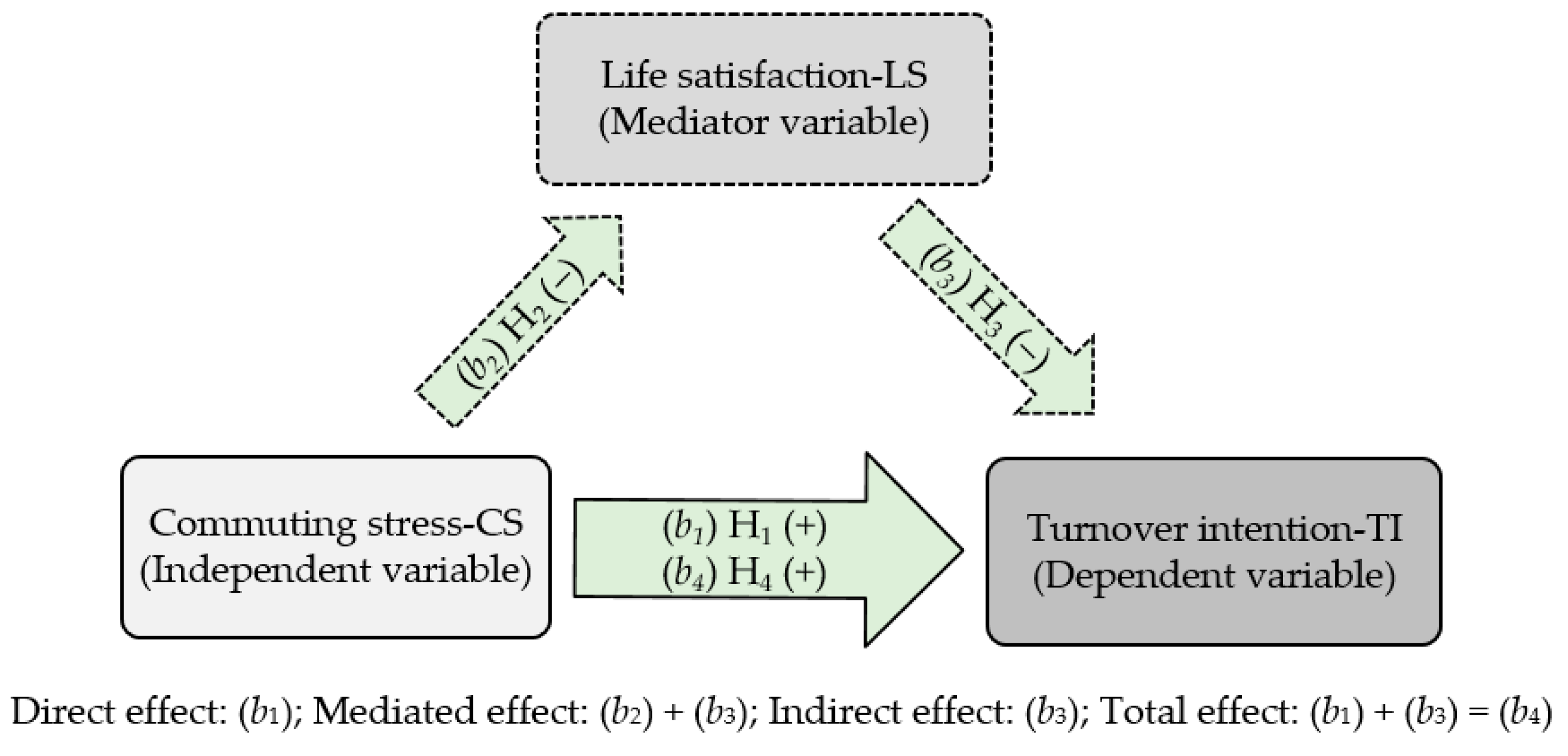
1
Alternatively, mediation studies have been also using structural equation modeling, which combines factor analyses, path diagrams, and a system of linked regression equations to capture complex and dynamic relationships within a web of observed and unobserved (latent) variables that can simultaneously be both dependent and independent variables. In our case, because there were only three variables and a clear distinction existed between the dependent and independent variables with causal relationships rather than casual linkages, the hierarchical regression analysis was more appropriate.
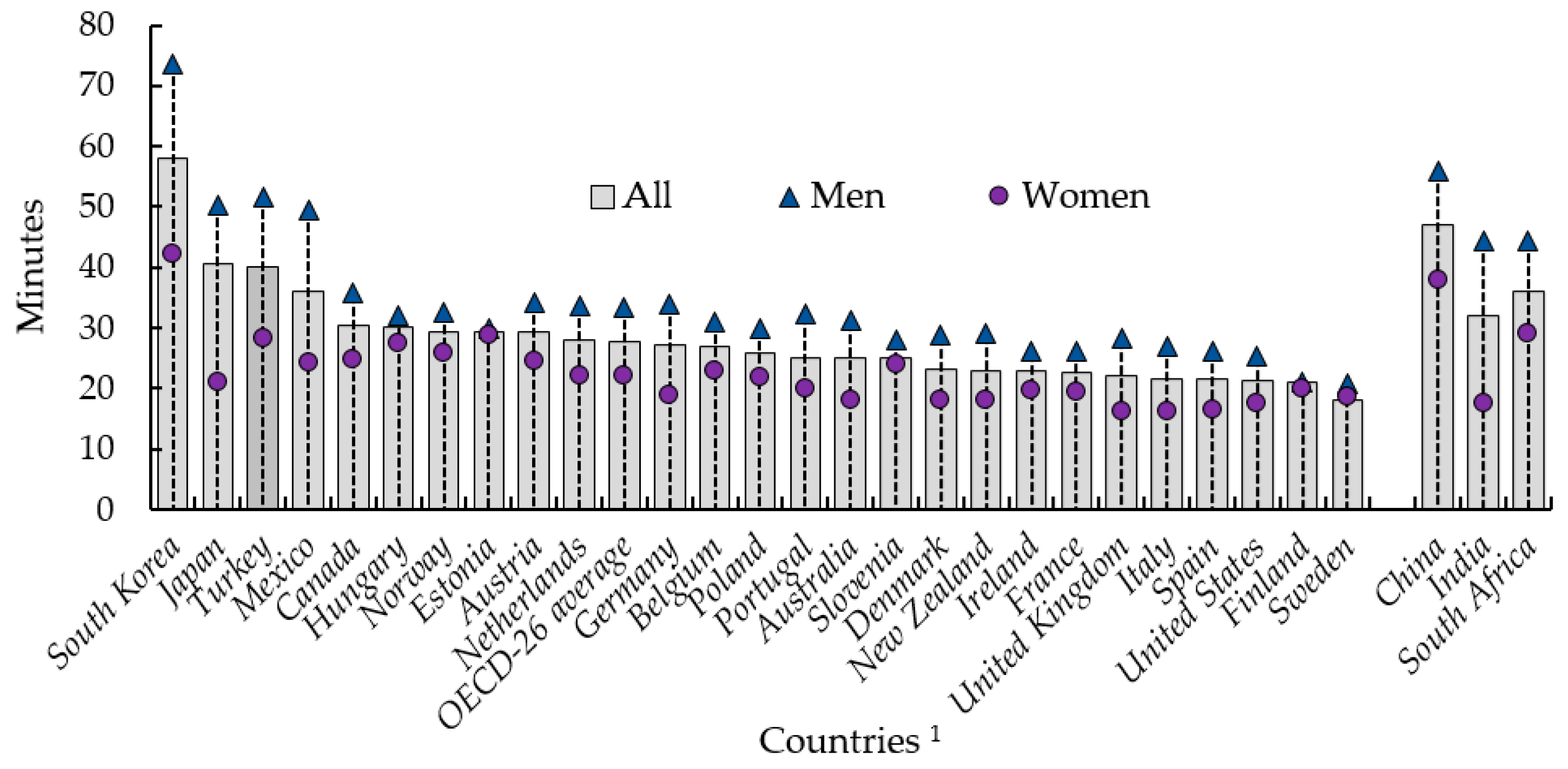
2
This vacation congestion is another cause of the increase in the CS of summer workers, especially in coastline cities.
Figure 1. Average daily commuting time in OECD countries and China, India, and South Africa.
Socsci 07 00147 g001
Figure 2. The hypothesized mediation model for the study.
Socsci 07 00147 g002
Table 1. Organizational causes of turnover intention (TI) and their presumed effects.
AspectStatementEffect
PaymentThe money paid to employees for the services and values they add.
IntegrationHaving close friends and good relationships with colleagues at work.
Internal communicationThe extent to which employees have efficient and sustained communication with colleagues at work.
External communicationThe extent to which employees have efficient and sustained communication with their counterparts in other organizations.+
CentralizationThe extent to which organizational decisions are often made by employers or by empowered and privileged several managers.+
RoutinizationThe extent to which job-related responsibilities are repetitive.+
Distributive justiceThe prevalence of a merit and performance-based promotion system.
Upward mobilityThe possibility and availability of movement between different status and career levels in organizations.
Job satisfactionThe extent to which employees are satisfied with what they do.
Work commitmentThe extent to which employees feel committed to their work.
Occupational statusThe extent to which employees hold occupational status.
Source: Author’s adaptation from Martin (1979) and Moynihan and Pandey (2008).
Table 2. Environmental and individual causes of turnover intention (TI) and their presumed effects.
AspectStatementEffect
OpportunityThe availability of alternative occupational roles and job opportunities offered by other organizations in the working environment+
Social networksIntra-organizational social network
Inter-organizational social network+
Social/community networks+
CommutingLocation of work (distance to home)+
Location of home (distance to work)+
Length of serviceThe time that employees have been working at the company
AgeElder employees are more inflexible and thus loyal to their organizations
Education and trainingAlthough more educated and trained employees are expected to be more flexible, education and training qualifications should be considered+
Gender and marital statusShould be considered together with other demographics and cultural values+/−
Work typeThe effects of working as blue or white collar are inconclusive+/−
Source: Author’s compilation based on the predominant evidence of previous studies.
Table 3. How and how long participants usually commute (regarding the last two years) (N:214).
Commuting Type
Driving aloneCarpoolingPublic transportationWalkingBicycle/motorcycleTelecommutingTotal
100413921211214
47%19%18%10%1%5%100%
Round-trip duration of commuting (in minutes)
20−20–4040–6060–8080–100100+Total
484250341921214
22%20%23%16%9%10%100%
Table 4. Characteristics of 29 businesses (N:214).
CategoryGroupNo. of Businesses (and %) (1)No. of Respondents (and %) (1)
Business sectorManufacturing16 (55)113 (53)
Service7 (24)60 (28)
Trade6 (21)41(19)
Location (City)İstanbul14 (48)110 (51)
Ankara5 (17)36 (17)
İzmir4 (14)29 (14)
Adana2 (7)13 (6)
Antalya2 (7)14 (7)
Mersin2 (7)12 (6)
Business size
(no. of total employees)
Small: 5–197 (24)20 (9)
Medium: 20–9911 (38)79 (37)
Large: 100+11 (38)115 (54)
(1) Due to rounding to the nearest whole, some percentages cannot add up to 100.
Table 5. Demographics of respondents (N:214).
CategoryGroupFrequency%
Age20–294220
30–396932
40–496028
50+4320
GenderMale13563
Female7937
Marital statusSingle(1)7133
Married14367
Number of childrenNone8339
14119
26229
3 and more2813
Formal education levelElementary school degree2411
High school degree7937
Bachelor’s degree8339
Master’s degree188
Doctoral degree105
Time in current job
(job tenure)
2 years or less3617
3–5 years6631
6–8 years5425
9 or more years5827
Time at company (organizational tenure)5 years or less7836
6–10 years8037
11 or more years5626
Job statusPermanent18687
Contract2813
Managerial positionWhite collar(2)11956
Blue collar(3)9544
(1) Divorced, separated or widowed participants were included in the single people group. (2) White-collar employees are those who usually perform job duties in an office setting. (3) Blue-collar employees are those who usually perform labor jobs and typically work with their hands.
Table 6. Final items of the commuting stress (CS) scale and their standardized factor loadings.
ItemsFactor Loading
It takes me longer than necessary to commute to work in the morning.0.83
It takes me longer than necessary to commute back home after work.0.80
I am unable to avoid heavy traffic on my way to work.0.72
I am unable to avoid heavy traffic on my way back home after work.0.76
I have to leave home earlier than I would like because of traffic congestion.0.68
Traffic congestion is a frequent inconvenience.0.65
My journey to and from work is often interrupted by traffic signals.0.71
I am not satisfied with my journey to and from work.0.80
My journey to and from work is unpleasant.0.87
I worry about my journey to and from work due to traffic accidents.0.66
Source: Excerpted from Amponsah-Tawiah et al. (2016).
Table 7. Final items of TI scale and their standardized factor loadings.
ItemsFactor Loading
If I had the chance, I would be working for another organization.0.83
I will probably look for other organizations to work for in the near future.0.77
I have never thought of leaving this organization(1).0.84
I feel a ‘strong’ sense of belonging to my organization(1).0.75
I feel ‘emotionally attached’ to this organization(1).0.79
I am loyal to this organization(1).0.73
I really feel as if this organization’s problems are my own(1).0.69
(1) Reverse-coded item. Source: The first two items were developed by the author, whereas the reverse-coded items were adapted from Allen and Meyer (1990).
Table 8. Final items of the life satisfaction (LS) scale and their standardized factor loadings.
ItemsFactor Loading
In general, I am satisfied with my housing expenditure and my dwelling’s basic facilities.0.68
In general, I am satisfied with my earning.0.73
In general, I am satisfied with my job quality.0.55
In general, I am satisfied with my social networks.0.58
In general, I am satisfied with my education.0.70
In general, I am satisfied with my environment regarding water quality and air pollution.0.63
In general, I am satisfied with the services provided by the local governmental institutions.0.52
In general, I am satisfied with the health services I am offered.0.59
In general, I am happy with my life.0.79
In general, I feel I am safe in my dwelling area.0.68
I think I can efficiently balance my working and personal lives.0.77
Source: Proposed by the author based on the OECD Better Life Index (2018).
Table 9. Comparison of mean differences in demographics: ANOVA F-test results (N:214). (CS: Commuting Stress, LS: Life satisfaction, TI: Turnover intention).
GroupsCSLSTI
Mean(1)FpMean(1)FpMean(1)Fp
Gender
Male (n:135)3.277.250.00 (5)3.991.930.173.480.860.36
Female (n:79)3.683.783.34
Marital status
Single (n:71)3.2111.590.00 (5)3.963.140.07 (3)3.524.950.03 (4)
Married (n:143)3.743.803.31
Age
20–29 (n:42)3.2811.430.00 (5)3.733.830.0143.470.280.83
30–39 (n:69)3.203.763.40
40–49 (n:60)3.583.953.36
50+ (n:43)3.824.093.42
Number of children
None (n:83)3.2012.350.00 (5)3.850.560.573.440.210.80
1–2 (n:103)3.633.823.38
3 and more (n:28)3.583.963.42
Commuting type (2)
Driving alone (n:100)3.462.920.04 (4)3.890.190.903.592.840.04 (4)
Carpooling (n:41)3.393.863.36
Public transportation (n:39)3.703.833.41
Other (n:34)3.323.923.30
Commuting duration
<20 (n:48)2.9435.700.00 (5)3.870.810.513.422.810.03 (4)
20–40 (n:42)2.913.763.17
40–60 (n:50)3.483.943.48
60–80 (n:34)3.833.993.45
80+ (n:40)4.213.873.59
(1) Comparisons are based on the means of two survey responses. (2) Together with walkers and bicycle/motorcycle riders, 11 employees working out of the workplace (telecommuting) were also included in the ‘other’ commuter group, since they declared that they sometimes stopped by their organizations and traveled between places to fulfill their job-related tasks. (3) Statistically significant at the level of 10%. (4) Statistically significant at the level of 5%. (5) Statistically significant at the level of 1%.
Table 10. Tukey HSD (honestly significant difference) test results (1). (CS: Commuting stress, LS: Life satisfaction, TI: Turnover intention).
Group PairMeansQ Statisticp
AgeCS
(20–29) vs. (40–49)(3.28) vs. (3.58)3.480.07 (2)
(20–29) vs. (50+)(3.28) vs. (3.82)5.880.00 (4)
(30–39) vs. (40–49)(3.20) vs. (3.58)5.010.00 (4)
(30–39) vs. (50+)(3.20) vs. (3.82)7.510.00 (4)
AgeLS
(20–29) vs. (50+)(3.73) vs. (4.09)3.940.03 (3)
(30–39) vs. (50+)(3.76) vs. (4.09)4.020.02 (3)
No. of childrenCS
(None) vs. (1–2)(3.20) vs. (3.63)6.850.00 (4)
(None) vs. (3 and more)(3.20) vs. (3.58)4.040.01 (3)
Commuting typeCS
(Carpooling) vs. (Public transportation)(3.39) vs. (3.70)3.330.09 (2)
(Public transportation) vs. (Other modes)(3.70) vs. (3.32)3.830.04 (3)
Commuting typeTI
(Driving alone) vs. (Other modes)(3.59) vs. (3.30)3.410.08 (2)
Commuting durationCS
(20−) vs. (40–60)(2.94) vs. (2.91)6.220.00 (4)
(20−) vs. (60–80)(2.94) vs. (3.83)9.240.00 (4)
(20−) vs. (80+)(2.94) vs. (4.21)13.780.00 (4)
(20–40) vs. (40–60)(2.91) vs. (3.48)6.340.00 (4)
(20–40) vs. (60–80)(2.91) vs. (3.83)9.290.00 (4)
(20–40) vs. (80+)(2.91) vs. (4.21)13.710.00 (4)
(40–60) vs. (60–80)(3.48) vs. (3.83)3.670.08 (2)
(40–60) vs. (80+)(3.48) vs. (4.21)8.020.00 (4)
(60–80) vs. (80+)(3.83) vs. (4.21)3.790.06 (2)
Commuting durationTI
(20–40) vs. (80+)(3.17) vs. (3.59)4.530.01 (3)
(20–40) vs. (40–60)(3.17) vs. (3.48)3.460.10 (2)
(1) Only significant comparisons are shown. (2) Statistically significant at the level of 10%. (3) Statistically significant at the level of 5%. (4) Statistically significant at the level of 1%.
Table 11. Descriptive statistics and correlation matrix. (CS: Commuting stress, LS: Life satisfaction, TI: Turnover intention).
First Survey (Conducted in Winter)Second Survey (Conducted in Summer)
CSLSTICSLSTI
Mean3.32 (1)3.933.383.633.843.46
Maximum7.007.007.007.007.007.00
Minimum1.001.001.001.001.001.00
Std. Dev.1.521.391.731.471.461.68
Skewness0.310.380.490.380.300.51
Kurtosis2.552.422.272.672.492.31
CS1.00 1.00
LS−0.27 (2)1.00 −0.33 (2)1.00
TI0.44 (3)−0.29 (2)1.000.51 (3)−0.34 (2)1.00
Observations (N) 214214
(1) Significantly (p < 0.01) lower than that of in the second survey. (2) Correlations are bilaterally significant at the level of 5%. (3) Correlations are bilaterally significant at the level of 1%.
Table 12. Estimated causal relationships between CS, LS, and TI (N:214). (CS: Commuting stress, LS: Life satisfaction, TI: Turnover intention).
ModelCausal PathStandardized Coefficient (1)ConstantFR2Durbin–Watson Stat.
1CSTI0.53
(0.07) [7.72] (2)
1.56
(0.26) [5.95] (2)
59.610.221.78
2CSLS−0.28
(0.07) [4.30] (2)
4.83
(0.25) [19.35] (2)
18.490.081.82
3LSTI−0.32
(0.08) [−4.30] (2)
4.71
(0.31) [15.14] (2)
18.480.081.62
4CS; LSTI0.48
(0.07) [6.76] (2);
−0.19
(0.07) [−2.62] (2)
2.49
(0.43) [5.72] (2)
34.070.251.76
(1) Standard errors and t-statistics of coefficients are respectively denoted in (parentheses) and [brackets]. (2) Statistically significant at the level of 1%.
Table 13. Control for model specification error: comparisons of model alternatives. (CS: Commuting stress, LS: Life satisfaction, TI: Turnover intention).
Suggested and Estimated Models of the StudyModel Alternatives
Dependent VariableIndependent Variable(s)R2Dependent VariableIndependent Variable(s)R2
TICS0.22CSTI0.09
LSCS0.08CSLS0.02
TILS0.08LSTI0.01
TICS, LS0.25CSTI, LS0.11
LSTI, CS0.14
Table 14. Bootstrap estimation of the mediating effect of LS on the CS–TI relationship (N:1000). (CS: Commuting stress, LS: Life satisfaction, TI: Turnover intention).
Causal PathCoefficient (Average)Std. ErrorConfidence IntervalInference
LowerUpper
CSTI0.610.090.040.15Significant at the level of 5%.
CSLS−0.300.090.040.14
LSTI−0.240.110.060.15
CS; LSTI0.45; −0.160.10; 0.090.050.13

