1. Introduction
Over the past decades, scholars are eager to understand and exploit the structural properties of networks such as social, ecological, disease, transportation, biological, information networks, and so on. Apparently, the better we understand the features of these networks, the more benefits we will obtain by applying these features in real world practices. The modern study of networks is fundamentally concerned with defining complex networks that occur in reality, in the hopes of better understanding their properties. Incidentally, since networks may be defined to represent a multitude of different scenarios, the study of networks has implications across a broad range of research interests. According to
Jackson (
2010b), the interdisciplinary application of network structure is what makes the scientific study of networks possible. Even further,
Jackson (
2010b) claims that the profound impact that networks have on the behavior dynamics of a system is what makes the study of networks a necessity.
A brief synopsis of the major areas of application for the study of networks may be found in (
Chakrabarti and Faloutsos 2012). Among others, social networks are perhaps most prevalent today in terms of online networks such as Facebook, Twitter, LinkedIn, etc. From a standpoint of modelling, within a society, social networks may be depicted to represent any collection of human entities and their associated connections. Cyber-security utilizes network analysis to identify abnormal behavior or anomalies within the system as a way to enhance protection. Website organization, the linking of websites to other websites first examined by
Barabasi et al. (
2000), can be represented as a complex network. Moreover, search engines must be able to navigate these networks efficiently. Influence propagation is a type of network study related to increasing the spread of information and/or ideas. On the other hand, this is also the area of interest concerned with stopping the spread of negative entities such as diseases or computer viruses. Finally, protein–protein interactions in biology have become a well-documented case for the application of complex networks.
This paper is concerned with modelling and simulation of the formation of networks. Simulation studies are commonly conducted to investigate into the dynamics of complex networks (
Zeng et al. 2013).
Chakrabarti and Faloutsos (
2012) refer to work of this kind as the simulation of synthetic graphs, along with the identifying certain properties within such networks. Synthetic graphs are generally constructed to give new insight regarding the properties of a specific network type. According to
Watts and Strogatz (
1998), real-world networks are neither completely ordered nor are they completely random, but rather lie somewhere along the spectrum between these two extremes. Therefore, the application of synthetic networks to reality may not be clearly defined until some realistic network is shown to share properties that align with that of the synthetic. We may only operate under the condition that such research will be used in the motivation for further network study.
The study of network formation has been actively carried out for the past decades. Considerable discussion on modelling network formation may be found in the literature (
Jackson 2010a;
Jackson 2005a;
Jackson 2005b;
Jiang et al. 2015). Most notably, the majority of the work consider systems of
undirected graphs. We note that our study adopts similar approaches to network formation modelling. More specifically, the formation of a network is represented by the construction of the network that typically goes as follows. One assumes that there exists one node at time zero (
t = 0) in the network. A new node is then born into the network corresponding to a discrete date in time,
t (
t = 1, 2, …). Consequently, the number of nodes in the network grows by one for every date that passes. Let
i represent an individual node within the network where
i is defined to be the time at which the node is born. Labeling nodes in this manner allows one to index individual nodes by the time at which they are born. For example, node
i (
i = 1, 2, …) is born when the network is at time
t =
i; one may label the initial node 0 for that matter. Each time when a newborn node has been introduced into the network, the newborn node may make connections with a number of nodes chosen in accordance with some pre-specified condition from the nodes that are already present in the network. That is, an edge is added to the network to connect the newborn node and each chosen node. This construction process continues indefinitely (
). The network grows following typically a slow Markov chain. One may then be interested in some asymptotic properties of the resulting network. For example, one may want to investigate into the distribution of degree of a node in the network. The degree of a node refers to the number of edges (connections) emanating from the node. In a practical sense, the degree of a node may be thought of as the number of acquaintances an individual has in a friendship network.
Barabasi and Albert develop a model based upon the above-described process (
Barabasi and Albert 1999). In their models, a newborn node leverages a condition called preferential attachment to make connections with chosen existing nodes. Specifically, the new node forms a
fixed number of edges with existing nodes. An existing node is randomly chosen with a probability proportional to the number of edges that the existing node currently has. For example, if an existing node has twice as many edges as does some other node, then this existing node is twice as likely to get connected with the new node. Employing the notion of mean-field approximation, they determine that the distribution of degree of a node for their model is a power-law distribution. A node degree distribution of this kind is typically characterized with a fat tail. Their results are clearly an approximation since a power-law distribution is a continuous distribution; however, the degree of a node is obviously discrete, nonnegative integer-valued. More recently,
Hamdi and Krishnamurthy (
2012) utilize novel stochastic approximation algorithms to estimate the degree of each node in social networks. We note that results in this field of study have been all presented in continuous distributions. This is definitely a glaring deficiency.
Our study differs from that of Barabasi and Albert in a significant way. In our models, a newborn node makes a
random number of connections with nodes that are already present in the network; every existing node may be
equally likely chosen by the newborn node. As an example, when a node is newly introduced into the network, the node may then, with probability 0.30, connect with a node chosen equally likely from the existing pool of nodes; or, with probability 0.70, connect with two nodes chosen equally likely from the existing pool. The objective of the study is to determine the distribution of degree of a node in such a network. We note that our results are presented in discrete distributions; this is a notable step forward in this area of research. To the best of our knowledge, there has not been any work conducted in this regard. A practical scenario for our models might be that a new member in a club may make acquaintance with a random number, rather than a fixed number, of existing members. For example, an individual may tend to more likely (less likely) make acquaintance with other individuals having similar (dissimilar) backgrounds, ages, interests, personalities, hobbies, and the likes, on Facebook, Twitter, LinkedIn, etc. As another example, users in trust networks can trust only the users whom they know and then some sort of randomness on the number of acquaintances may be assumed (
Meo et al. 2017;
Golbeck et al. 2003;
Yuan et al. 2010). One may then be interested in gaining insight into the number of acquaintances a member has in the club.
We present the remainder of the paper as follows.
Section 2 provides a brief overview of existing results in related work.
Section 3 formally defines our models, finds solutions, and discusses examples. Finally, concluding remarks are offered in
Section 4.
2. A Brief Overview of Existing Results on the Distributions of Node Degree
This section provides a brief overview of how some of the existing work in the literature models the formation of social networks. We note that researchers in this area of work largely employ the notion of mean-field analysis (
Barabasi and Albert 1999) to derive the distributions of node degree for generated networks. As a consequence, results are presented in continuous approximations. These results may not be practical since the degree of a node ought to be nonnegative integers. To resolve this predicament, we endeavor to convert such results to their discrete analogues.
2.1. The Distribution of Degree of a Node in a Social Network
Consider a scenario in which a new member joining a club would randomly make acquaintance with a number of members who are already present in the club. One may be interested in gaining insight into the number of other members with whom a club member is acquainted in the club. From the network formation modelling perspective, such is equivalent to a newborn node making connections to a number of randomly chosen existing nodes in the network. One may then want to study the distribution of degree of a node in this network. We take a closer look at the degree growth process of a node in the network.
The degree growth process of a node in a network as the network grows may be divided into two parts. When a node is newly born into the network, the node makes a number of connections to nodes randomly chosen from the existing pool of nodes in the network. We term this process the initial process, and the number of connections the node makes at birth is considered as the initial degree of the node. Thereafter, this node may or may not be randomly chosen by a subsequent newborn node in the course of the network growth. If this node is chosen by a newborn node, this node now receives a connection from the newborn node and hence increases the number of connections (edges) by one; the number of connections of this node does not increase if this node is not chosen. We term this process the random process, and the number of connections this node receives in this random process is considered as the random degree. As a consequence, the (total) degree of this node in the network is essentially the sum of its initial degree and its random degree.
Bishop establishes the distribution of degree of a node in a network when the network grows sufficiently large (
Jackson 2005a). Specifically, let n be the constant number of connections a newborn node makes to (n) equally likely chosen nodes that are already present in the network. Bishop approximates, using the notion of mean-field analysis, that the random degree a node receives in the random process is exponentially distributed with mean equal to μ
0. In this case, one may obtain that μ
0 =
n. To see this, recall that each node is introduced into the network at a point in time, by time t in the network, there are a total of t existing nodes and there are a total of
nt edges (since n edges are added to the network each time a new node is introduced); therefore, the average number of edges a node in the random process may acquire in the long run is μ
0 =
. Bishop further determines that incorporating the initial degree given to a node in the initial process, in this case,
n, into the above-mentioned exponential distribution results in a shift to the right by
n units of the exponential distribution. Such is true in that each node in the network has at least degree n, the initial degree, and that the degree of each node grows as the node may be chosen by a newborn node in the random process. In sum, letting
K be the degree (initial degree plus random degree) of a node in the network, Bishop has found that
K is a shifted exponential random variable with the following probability density function,
The above result may not be practical since the degree of a node ought to be a nonnegative integer. However, such is usually considered as an approximation to the distribution of node degree and left as it is in the literature. To make a better sense of Equation (1), we therefore endeavor to convert it to a geometric distribution since it is common knowledge that the discrete analog of the exponential distribution is the geometric distribution.
2.2. The Discrete Analog of the Exponential Distribution
This subsection deals with converting the exponential distribution to its discrete analog.
Consider a nonnegative real-valued random variable
X. Assume that
X has the following probability density function and cumulative density function, respectively,
and
As such,
X is simply an exponential random variable with mean
E(
X) =
µ0. Let us imagine slicing the area under the graph of
f(
x) into vertical bars of width
a such that the area of the first bar is equal to
F(
a) −
F(0) =
; the area of the second bar,
F(2
a) −
F(
a) =
; the area of the third bar,
F(3
a) −
F(2
a) =
; and so on (
Teague 2015;
Bain and Engelhardt 1992). In general, the area of the
nth bar,
n = 0, 1, 2, …, is given by (note that we use
n = 0 to mean the first bar,
n = 1 to mean the second bar, etc.)
The above discussion underlies a geometric distribution. Suppose that
Y is a nonnegative integer-valued random variable. Further suppose that
P(
Y = 0) is equal to the area of the first bar; that
P(
Y = 1), the area of the second bar, that
P(
Y = 2), the area of the third bar; and so forth. Then, Equation (2) yields
where
q =
,
p =
, and
y = 0, 1, 2, … It is now obvious that
Y is a geometric random variable whose probability of success is
p =
and probability mass function is Equation (3). It follows that the mean of
Y is
E(
Y) =
=
We want random variable
Y to closely trail random variable
X. To this end, we equate the means of the two random variables, resulting in
Solving the above equation for
a gives rise to
Such suggests that in order for
Y to share the same mean as that of
X, one should set the width
a of each bar equal to
. By so doing, the probability of success for
Y is now
and
q =
. In a nutshell, the discrete analogue, sharing the same mean, of an exponential distribution with mean
µ0 is the geometric distribution with probability of success
.
2.3. The Discrete Distribution of Degree of a Node in a Social Network
We are now in a position to determine a discrete analog of Equation (1).
Let us visit the results established by
Bishop (
2014) and discussed in
Section 2.1. The random degree of a node acquired in the random process is exponentially distributed with mean
n, as approximated by Bishop. Drawing upon the results from
Section 2.2, one may now infer that the discrete random degree (say,
Y), having the same mean
n (hence,
µ0 =
n) for the discrete random degree associated with the same random process, is geometrically distributed with probability of success
. Furthermore, adding the initial degree
n obtained in the initial process to the node moves the geometric distribution to the right by
n units. Therefore, if
K is the total degree of the node in the network, we now have that
K (
K =
Y +
n) is a shifted geometric random variable with the following probability mass function,
where
p =
,
q =
, and
In summary, one may now readily conclude that Equation (5) is a practically meaningful distribution of degree of a node in a network in which a newborn node makes connections to
n equally chosen nodes that are already present in the network. On the other hand, Equation (1) is an approximation to the said distribution.
A close reading of the literature reveals that the study of network formation has thus far primarily been focused upon that a newborn node makes connections to a constant number of randomly chosen existing nodes in the network. However, more practically, it may not be unusual that a new member joining a club may wish to make acquaintance with a random number of randomly chosen existing club members. Under such circumstances, one may wish to gain insight into the number of other members with whom a club member is acquainted in the club. Such is equivalent to determining the distribution of degree of a node in a network in which a node makes at-birth connections to a random number of randomly chosen nodes that are already present in the network. To the best of our knowledge, no work to date has been conducted with such network formation scenarios. In the sequel, we seek to find the distribution of degree of a node in a network built under these scenarios.
3. Social Network Formation with a Random Number of Initial Connections
This section delves into the distribution of degree of a node in a network formed with a random number of initial connections from a node when the node is first introduced into the network. For example, new club members, more realistically, may want to make acquaintance with a varying number, rather than a fixed number, of randomly chosen members who are already present in the club. Such may be true in that an individual may tend to more likely (less likely) make acquaintance with other individuals having similar (dissimilar) backgrounds, ages, interests, personalities, hobbies, and the likes, on Facebook, Twitter, LinkedIn, etc. As another example, one is more likely (less likely) to connect with someone whom they trust more (less). Specifically in this section,
Section 3.1 formally presents our models;
Section 3.2 seeks to find solutions to our models. Then, in
Section 3.3, we will provide numerical examples to verify results established in
Section 3.2.
3.1. Our Models
We consider here a network being constructed in the following fashion. As a new node is introduced into the network, a number, determined by chance, of nodes that are already present in the network are equally likely chosen. An edge is then added between the new node and each of the chosen nodes. This process is repeated indefinitely. As an example, a newborn node, with a 30% chance, may connect to one equally likely chosen existing node; and, with a 70% chance, may connect to two equally likely chosen existing nodes. This process may repeat as many times as we wish. The objective is to determine the distribution of degree of a node in such a network.
We use a positive integer-valued random variable to represent the random number of nodes equally likely chosen from the pool of existing nodes by a node at the time when it is born into the network. Let
K be this random variable. We may then specifically define the probability mass function of
K in the following
Table 1. That is, a newborn node may connect to
k1 equally likely chosen existing nodes with probability
p1; to
k2 equally likely chosen existing nodes with probability
p2; and so on. We note that
ki, with
i = 1, 2, …,
n, are positive integers, and that
. Of great interest to us then is the number of other nodes to which a node connects as the network becomes sufficiently large.
3.2. Determine the Distribution of Degree of a Node with a Random Number of Initial Connections
This section seeks to determine the distribution of degree of a node in the model presented in the preceding section. To this end, let
μ0 =
E(
K) =
k1p1 +
k2p2 + …... +
knpn. Observe that
μ0 is the average number of edges a node may acquire in the random process. To see this, each new node at birth adds, on average, (
k1p1 +
k2p2 + …... +
knpn) edges to the network. By time
t, there are a total of
t existing nodes and hence there are a total of (
k1p1 +
k2p2 + …... +
knpn)
t edges in the network; thus, the average number of edges a node in the random process may acquire in the long run is
. Drawing upon the results presented in
Section 2, we are now in a position to further determine the distribution of degree of a node in the network.
Consider a node chosen at random from the network. Let
K0 represent the number of edges (random degree) the node acquires in the random process. Then,
K0 is a geometric random variable, with probability of success
, having the following probability mass function,
where
p =
,
q =
, and
Now assume that this node makes at its birth
ki (
i = 1, 2, …,
n) connections (initial degree) to equally likely chosen existing nodes in the initial process. Then, if
Ki represents the total degree (initial degree plus random degree) the considered node possesses,
Ki (
Ki =
K0 +
ki) is a shifted geometric random variable resulted from moving
K0 by
ki units to the right. Consequently, the probability mass function of
Ki is
where
p =
,
q =
, and
One may in fact visualize that there are n types of nodes in the network. That is, nodes of Type i are the nodes whose initial degree is ki (i = 1, 2, …, n). Subsequently, the degree of a node of Type i is represented by Ki. Notably, as the network becomes sufficiently large, one may consider that the proportion of Type i nodes is approximately pi, and that types of nodes are nearly independent. As it turns out, our results reflect that this consideration is indeed warranted. Therefore, choosing randomly a node from the network is not very much unlike drawing at random an individual from a population comprising multiple subpopulations. Such underlies the basis of determining the distribution of degree of a node in the network.
The following proposition establishes that the degree of a node in a network as constructed in accordance with
Section 3.1. To this end, we first assume that
= min{
k1,
k2, ...,
kn}; that
k =
,
+ 1,
+ 2, ...; and that
Ii(
k) = 1 if
k ≥
ki and
Ii(
k) = 0 if
k <
ki (
i = 1, 2, …,
n). Finally, suppose that
represents the total degree (initial degree plus random degree) of a node in the network. We now state and prove the proposition as follows.
Proposition 1. The degree of a node in a network as constructed in accordance with Section 3.1 is a mixture. Specifically,
= KI with P(I = i) = pi, i = 1, 2, …, n. Furthermore, the probability mass function of is where p =
,
q =
,
and k =
,
+
1,
+ 2, … Proof of Proposition 1. The degree
of a node in a network as constructed in accordance with
Section 3.1 is a mixture. To see this, one may visualize that the network is composed of a population of roughly independent nodes, as the network becomes sufficiently large. Moreover, there are
n nearly independent subpopulations. A subpopulation
i is a set of nodes with initial degree being
ki; and designates a node of subpopulation
i as a node of Type
i (
i = 1, 2, …,
n). The fraction of Type
i nodes in the network is approximately
pi; the degree of a Type
i node is represented by
Ki. Therefore, the degree
of a node chosen at random from the network is then a mixture
=
KI with
P(
I =
i) =
pi, i = 1, 2, …,
n, since the chosen node is of Type
i with probability
pi. Now, to determine the probability mass function of
, we invoke the Law of Total Probability to have
where
p =
,
q =
, and
k =
,
+ 1,
+ 2, … The proof has now been completed. ☐
The above proposition provides us with a theoretical means to approximate the distribution of degree of a node in a network considered in the study. It does not come as a surprise that such approximations yield desirable results as the network becomes sufficiently large. The next section presents three numerical examples to demonstrate the goodness of the proposition.
3.3. Numerical Examples
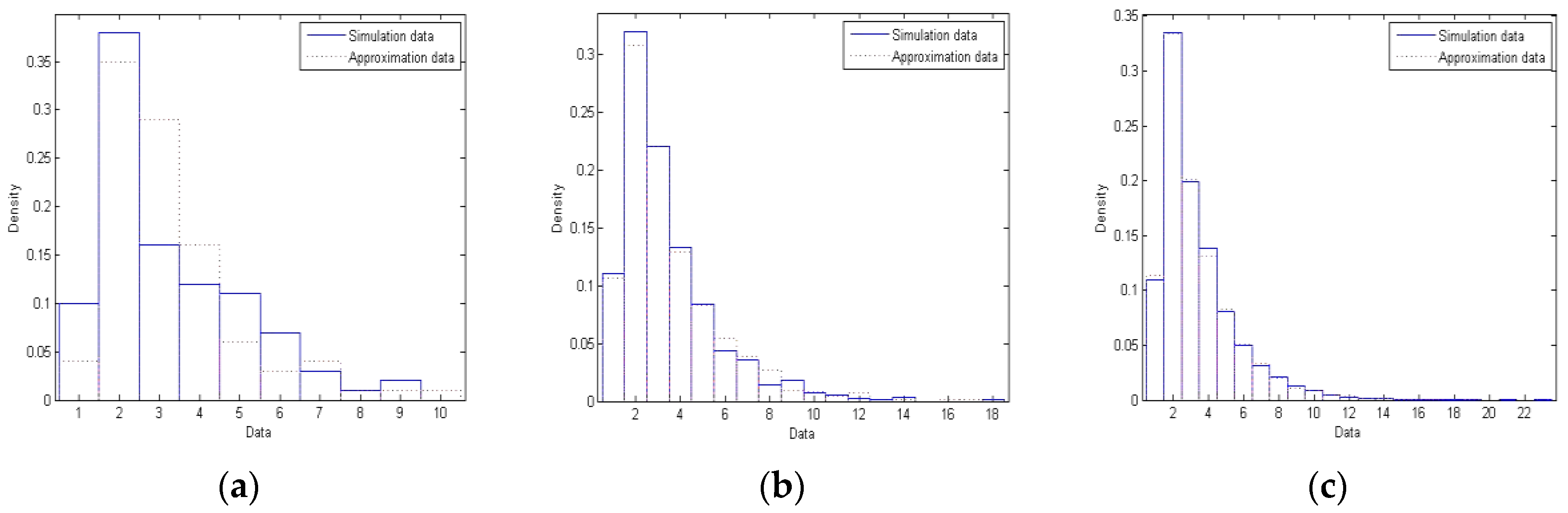
The section presents three numerical examples to show the goodness of Proposition 1 established in the previous section. In each example, we conduct the following study. A simulation program coded in MATLAB is leveraged to build networks of different sizes as our models. The size of a network refers to the number of nodes in the network. We look into networks with three different sizes. For each network, a probability histogram (percent of nodes versus degree) is constructed; we dub this “Simulation” data. One the other hand, another probability histogram (percent of observations versus observation) is created, only this time around, employing observations randomly drawn from the mixture established in Proposition 1; we dub this “Approximation” data. These two histograms are overlaid on each other for comparison. Specifically, blue solid lines represent Simulation data, while red dotted lines mean Approximation data.
We now look at our first example.
Table 2 shows the probability mass function of random variable
K representing the random number of initial connections for a newly born node. Most briefly, when a new node is introduced into the network, we, with probability 0.30, equally likely choose one existing node and then connect the new node and the chosen node with an edge (rendering initial degree 1 for the new node in this case). However, we, with probability 0.70, equally likely pick two existing nodes and then connect the new node and each of the chosen nodes with an edge (rendering initial degree 2 for the new node in this case). (We have alluded to this example before in the paper.) We note, in this example, that
μ0 =
E(
K) = 1(0.30) + 2(0.70) = 1.7, and hence that
p = 1/2.7 and
q = 1.7/2.7. We therefore have that
P(
K1 =
k) = (1.7/2.7)
k−1(1/2.7),
k = 1, 2, …, and that
P(
K2 =
k) = (1.7/2.7)
k−2(1/2.7),
k = 2, 3, … Finally, we have, as discussed in Proposition 1, the mixture
=
KI with
P(
I = 1) = 0.30 and
P(
I = 2) = 0.70.
We generate data as follows. First, a MATLAB program simulates the network construction, creating three networks of different sizes which are, for this example, 100, 1000 and 10,000 nodes. Then, for each network, the fraction of nodes of a certain degree is determined to establish a probability histogram; such is indicated as “Simulation” data. In the meantime, we draw randomly a set of observations, of the same size, from our mixture
. A similar histogram is subsequently constructed based upon this set of observations; such is presented as “Approximation” data. Finally, we superimpose these two histograms for comparison; we use blue solid lines to mean Simulation data and red dotted lines for Approximation data. Let us now take a look at
Figure 1. There are probability histograms (a), (b) and (c) for networks with 100, 1000 and 10,000 nodes, respectively. Specifically, Histogram (a) reveals that there are about 10 nodes of degree 1 in the simulated network (blue solid lines) while there are about 4 nodes of degree 1 in the random observations drawn from
(red dotted lines), that there are about 38 nodes of degree 2 in simulation while there are about 35 nodes of degree 2 in approximation, etc. We note that Histogram (a) may also be interpreted like this. A random node chosen from the network has a 10% chance of possessing degree 1 while a 38% chance of possessing degree 2, and so on, according to the simulation data; on the other hand, the said node has a 4% chance of possessing degree 1 while a 35% chance of possessing degree 2, and so on, based upon the approximation data. Lastly, it is evident that the simulation and approximation data match each other better as the size of the network grows larger from (a) to (c).
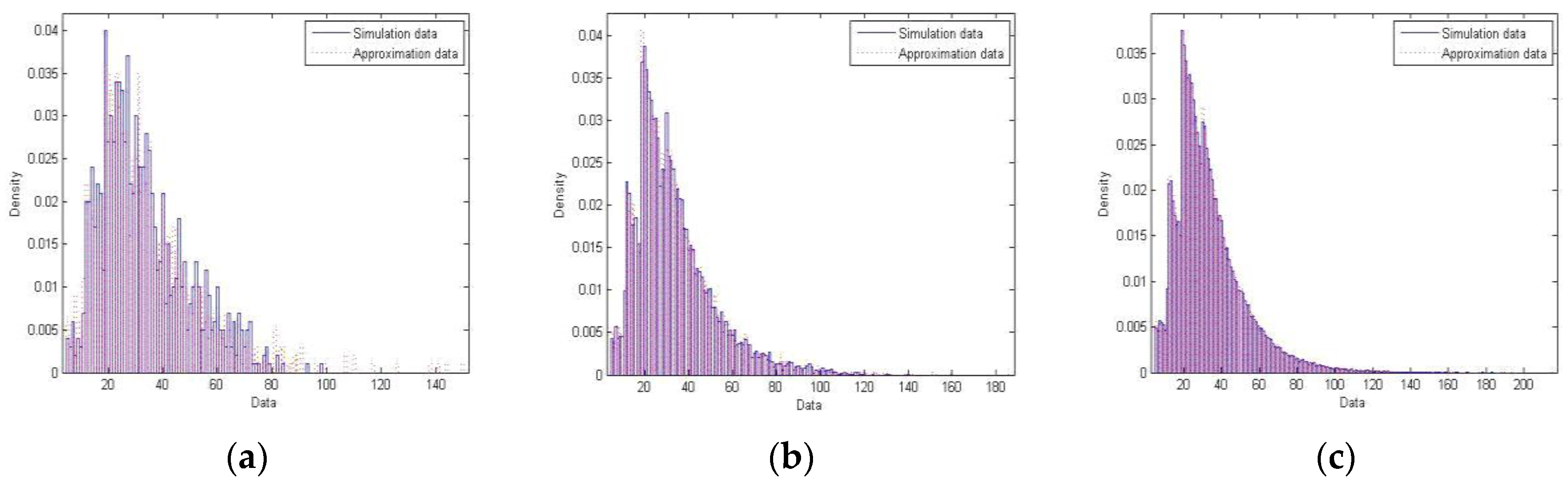
We next move on to the second example.
Table 3 contains the possible options for initial degree that a node of the considered network may be given. A quick arithmetic returns
μ0 = 9.55; such is employed to establish the desirable mixture
.
Figure 2 illustrates similar histograms for this second example. Since the initial degree options are more complex, we simulate three larger networks of sizes 1000, 10,000 and 100,000, respectively. Notice, as well, that the simulation and approximation data become closer to each other going from (a) to (c).
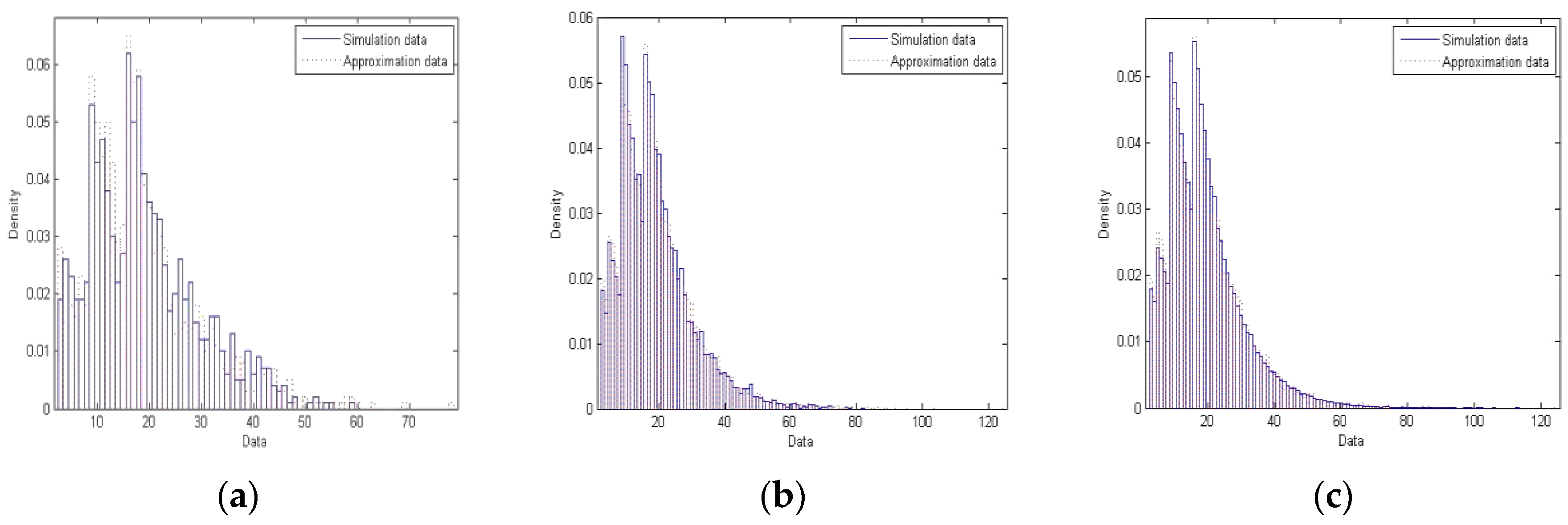
Let us finally talk about our last example, the third example. The initial degree of a node in this example is detailed on
Table 4. This example is characterized by highly varying initial degree with average being
μ0 = 16.66.
Results for this third example are illustrated in
Figure 3. The similarity between simulation and approximation is once again apparent.
The above examples clearly verify that the mixture found in Proposition 1 closely approximates the distribution of degree of a node in networks for which initial degree may be very much random.


